Improved African Vulture Optimization Algorithm for Optimizing Nonlinear Regression in Wind-Tunnel-Test Temperature Prediction

Abstract

The thermal data of the hypersonic wind tunnel field accurately reflect the aerodynamic performance and key parameters of the aircraft model. However, the prediction of the temperature in hypersonic wind tunnels has problems such as a large delay, nonlinearity and multivariable coupling. In order to reduce the influence brought by temperature changes and improve the accuracy of temperature prediction in the field control of hypersonic wind tunnels, this paper first combines kernel principal component analysis (KPCA) with phase space reconstruction to preprocess the temperature data set of wind tunnel tests, and the processed data set is used as the input of the temperature-prediction model. Secondly, support vector regression is applied to the construction of the temperature prediction model for the hypersonic wind-tunnel temperature field. Meanwhile, aiming at the problem of difficult parameter-combination selection in support vector regression machines, an Improved African Vulture Optimization Algorithm (IAVOA) based on adaptive chaotic mapping and local search enhancement is proposed to conduct combination optimization of parameters in support vector regression. The improved African Vulture Optimization Algorithm (AVOA) proposed in this paper was compared and analyzed with the traditional AVOA, PSO (Particle Swarm Optimization Algorithm) and GWO (Grey Wolf Optimizer) algorithms through 10 basic test functions, and the superiority of the improved AVOA algorithm proposed in this paper in optimizing the parameters of the support vector regression machine was verified in the actual temperature data in wind-tunnel field control.

1. Introduction

When conducting wind-tunnel tests, due to the complexity of the airflow in the wind-tunnel flow field, the interaction between the airflow and the aircraft model, as well as the influence of various environmental factors, the wind-tunnel test data are typically nonlinear time series. The study of time series began in 1927 when Yule invented the autoregression method [1]. Researchers have successively proposed research methods for univariate and multivariate time series [2]. For nonlinear time series, researchers have proposed the threshold autoregression method. The autoregressive conditional heteroscedasticity method and its improved methods, etc., are discussed in Tsay (1989) [3]. The most representative example is that of 2011, namely, Jones et al., who, for the hypersonic intermittent blowing wind tunnel, abstractly regarded the entire wind-tunnel system as three pressure-vessel units and constructed a nonlinear mathematical model about the dynamic change of temperature based on the principle of mass continuity of pressure vessels. This was to achieve precise and stable regulation of the air density, air flow velocity and air-volume flow rate in the wind tunnel [4]. The above-mentioned nonlinear prediction method belongs to parametric modeling. Essentially, it belongs to the same parametric modeling framework as the linear method. Its core defect lies in the lack of dynamic adaptability of the prior assumptions of the model structure, and the established model exhibits a limited generalization capability. In the practical application scenarios of temperature prediction in wind-tunnel systems, the characteristics of wind-tunnel systems are often formed by the combined action of multiple factors such as multi-physical field coupling, multi-scale effects, and non-stationary random disturbances. The traditional parametric model is limited by the subjective bias of expert experience, and its preset model structure makes it difficult to match the dynamic evolution of system characteristics in real time. When the system undergoes sudden parameter changes, structural variations or environmental disturbances, the mismatch degree between the prior assumed model structure and the actual system characteristics will increase significantly, resulting in a nonlinear growth trend of the model prediction error. Therefore, breaking through the parametric modeling approach and developing intelligent modeling methods with self-learning and self-evolution capabilities has become the key technical bottleneck for improving the predictive performance of wind-tunnel systems.

At present, data-driven time series prediction models have gradually grown and developed. Compared with traditional linear prediction models such as univariate linear regression and the multivariate autoregressive moving average, as well as some models that can only handle specific nonlinear forms, data-driven methods break the inherent constraints of the model structure and data characteristics, and have stronger nonlinear approximation capabilities. In the prediction of time series, by constructing advanced neural network models such as the Convolutional Neural Network (CNN), Fuzzy Neural Network (FNN), Wavelet Neural Network (WNN), Long Short-Term Memory (LSTM), and Spike Neural Network (SNNs), it has been possible to achieve high-precision fitting and prediction of time series [5]. However, in neural networks and their corresponding algorithms, sufficient data samples are required and the model convergence process is slow. For the characteristics of small sample size and the short-term nature of wind-tunnel test data, support vector regression is more suitable compared to neural-network prediction. The support vector regression method has a strict theoretical and mathematical basis and is highly robust. In the temperature prediction of wind tunnels, the prediction accuracy of support vector regression is improved through intelligent optimization algorithms [6].

Meanwhile, with the development of swarm-intelligence algorithms, researchers draw inspiration from the living habits of social animals in nature, thereby creating intelligent optimization algorithms for solving complex engineering problems [7]. The essence of intelligent optimization algorithms is to simulate the evolution laws of natural or social systems through randomized search strategies and to estimate the optimal or approximate optimal solutions of the objective function in the complex solution space [8]. Algorithms can be classified according to their different design principles. The Genetic Algorithm (GA) [9], Differential Evolution (DE) [10] and Evolutionary Strategy (ES) belong to evolutionary algorithms that drive the iterative optimization of populations through genetic operators such as selection, crossover and mutation [11]. The Ant Colony Optimization Algorithm (ACO) [12], Particle Swarm Optimization Algorithm (PSO) [13] and Artificial Bee Colony Algorithm (ABC) all belong to swarm-intelligence algorithms [14], and they solve complex tasks through information sharing and collaborative actions among individuals. Facing the nonlinear, multimodal and complex constraint conditions existing in practical engineering applications, higher requirements have been put forward for optimization algorithms.

This paper addresses the issues such as slow convergence speed and insufficient accuracy when dealing with nonlinear and complex problems in the African Vulture Optimization Algorithm. To enhance the algorithm performance, the improved African Vulture Optimization Algorithm based on chaotic mapping and the local search enhancement method is proposed. Meanwhile, aiming at solving the problem of difficult parameter-combination selection in support vector regression machines, the improved vulture algorithm was then applied to the parameter optimization of support vector regression for predicting the temperature in the wind-tunnel field. The improved regression model, by using vulture optimization algorithm, demonstrates the better prediction accuracy and the lowest error index, providing a solution for practical applications.

2. Basic Theory

2.1. Kernel Principal Component Analysis

Conducting kernel principal component analysis (KPCA) can achieve nonlinear dimensionality reduction of data sets. KPCA is usually used to handle linearly inseparable data sets [15]. For the wind-tunnel test dataset, a nonlinear mapping was first used to map all the samples in the dataset to a high-dimensional or even infinite-dimensional space, called the feature space, to make it linearly separable. Then, Principal Component Analysis (PCA) was performed for dimensionality reduction in this high-dimensional space [16]. Specifically, it can be expressed by taking the $l\times n$ dimensional temperature data matrix $X$ as the input space for nonlinear mapping, $\varphi$ for mapping the data sample $X=\left\{x_1,x_2,\dots ,x_n\right\}$ input space $X$ to the feature space $H$ and denoting the feature space $H$ as the $l\times d$ dimension. The mapped dataset $\varphi (x)=\left\{{\phi }_1,{\phi }_2,\dots ,{\phi }_d\right\}$ was obtained. At this point, the temperature dataset in this feature space had completed the centralization processing by default. It can be known that

$$\varphi (x_i)\varphi {(x_j)}^T=0$$

(1)

Among these terms, $i=1,2,\dots ,n$, $j=1,2,\dots ,n$ and $i\ne j$, and the superscript $T$ represents the transpose of the matrix.

PCA analysis was performed on the dataset $\varphi (x)$ and the covariance matrix $C$ was calculated:

$$C={\displaystyle \frac{1}{n}}{\displaystyle \sum _{i=1}^n\varphi (x_i)\varphi {(x_i)}^T}$$

(2)

Diagonal processing $C$ was carried out on the obtained eigenvalues $\lambda$ and the corresponding eigenvectors $V$, where the following relationship was satisfied:

$$C={\displaystyle \frac{1}{n}}{\displaystyle \sum _{i=1}^n\varphi (x_i)\varphi {(x_i)}^T}$$

(3)

Since $V\in span\left\{\varphi (x_1),\varphi (x_2),\dots ,\varphi (x_i)\right\}$, it can be known that there is a relationship ${\alpha }_1,{\alpha }_2,\dots ,{\alpha }_n$ among a set of coefficients:

$$V={\displaystyle \sum _{j=1}^n{\alpha }_j\varphi (x_j)}$$

(4)

$V$ was substituted into the characteristic Equation (3), and $\varphi {(x_k)}^T$, $k=1,2,\dots ,n$ were multiplied with both sides of the equation to the left simultaneously to obtain

$${\displaystyle \frac{1}{n}}{\displaystyle \sum _{i=1}^n{\alpha }_i}\varphi {(x_k)}^T\varphi (x_i)\varphi {(x_i)}^T\varphi (x_j)=\lambda {\displaystyle \sum _{i=1}^n{\alpha }_i}\varphi {(x_k)}^T\varphi (x_i)$$

(5)

Introducing the kernel function $K$ can obtain the non-zero characteristic solution of this problem. A kernel function $K_{ij}=(\varphi {(x_i)}^T\cdot \varphi (x_j))=K(X_i,X_j)$ of $n\times n$ was defined, and then Formula (5) could be simplified to

$$K\alpha =n\lambda \alpha$$

(6)

Meanwhile, to satisfy the default centralization assumption, the kernel matrix was adjusted to

$$\overline{K}=K-I_{n}K-K{I}_n+I_{n}K{I}_n$$

(7)

where ${\left(I_n\right)}_{ij}={\displaystyle \frac{1}{n}}$.

According to Formula (7), the kernel matrix $\overline{K}$ was obtained, $\overline{K}$, the eigenvalues $V$ and the eigenvectors of the matrix $\lambda$ were calculated, and the eigenvectors $\lambda$ were normalized:

$${\alpha }^{\left(k\right)}={\displaystyle \frac{1}{\sqrt{{\lambda }_k}}}{V}^{\left(k\right)}$$

(8)

The cumulative $B_1,B_2,\dots ,B_n$ contribution rate of the eigenvalues ${\lambda }_1,{\lambda }_2,\dots ,{\lambda }_n$ was calculated. According to the cumulative contribution rate $P$ of the principal components that had been set, when $B_K\ge P$, the $k$ principal component and the corresponding principal component ${\alpha }_1,{\alpha }_2,\dots ,{\alpha }_k$ should be selected. By calculating the projections of the original sample data in these selected principal component directions $Y$, the dimensionally reduced wind-tunnel temperature test dataset was obtained.

Among them, the kernel functions mainly choose polynomial kernel functions and Gaussian kernel functions [17]. This paper selects the Gaussian kernel function, and its expression is as follows:

$$K\left(x_i,x_j\right)=\exp \left(-{\displaystyle \frac{{‖x_i-x_j‖}^2}{2{\sigma }^2}}\right)$$

(9)

Among them, $x_i$, $x_j$ are two sample vectors in the input space, and $\sigma$ are the bandwidth parameters of the kernel function.

After performing KPCA dimension reduction on the wind-tunnel test data, the data was reconstructed through phase space. Phase Space Reconstruction (PSR), as the core link of chaotic time series analysis, is a key step to revealing the intrinsic dynamic characteristics of the system. Through precise phase-space reconstruction, a nonlinear prediction model of the system can be established, providing important theoretical support for the control and prediction of chaotic systems.

After performing KPCA dimension reduction on the wind-tunnel test data, phase-space reconstruction processing was carried out. Phase-space reconstruction (PSR) is the core link of chaotic time series analysis and a key step to revealing the inherent dynamic characteristics of the system. Through precise phase-space reconstruction, a nonlinear prediction model of the system can be established, providing important theoretical support for the control and prediction of chaotic systems. The reconstructed wind-tunnel test data were used as the input of the subsequent model. The test statistical sequence $\overline{S}(\tau )$, the maximum deviation $\Delta \overline{S}(\tau )$ and the indicators $S_{cor}(\tau )$ were drawn. The $\Delta \overline{S}(\tau )$ first minimum value was taken as the optimal time delay ${\tau }_d$, and the global minimum value $S_{cor}(\tau )$ was taken as the time window length ${\tau }_w$ of the time series. Through the delay time $\tau$ and embedding dimension $m$ a phase space that was the same as the original system in the topological sense was reconstructed to improve the adaptability of the prediction model for the wind-tunnel test data.

$${\tau }_w=(m-1){\tau }_d$$

(10)

2.2. Support Vector Regression

Support Vector Regression (SVR), as an extension of SVM in the field of regression, breaks through the limitation that traditional linear regression can only handle linear relationships. By introducing kernel techniques and nonlinear mapping mechanisms to achieve the precise modeling of complex nonlinear systems, SVR is one of the typical applications in SVM [18].

The essence of SVM is to look for a given sample $\left(x_i,y_i\right)\left(i=1,2,\dots ,H\right)$ set for the generalized linear classification of the superplane logarithm $S\left(x,y\right)=0$, in which $x_i$ is the $i$ dimension $H$ input vector, $y_i$ is the $i$ scalar output and $H$ is the number of the sample number [19].

Considering that the temperature data are nonlinear, it was necessary to transform the nonlinearity of the input sample space to a high-dimensional linear feature space and solve the nonlinear problem in this high-dimensional space. Then, in the SVR algorithm, the function model can be expressed as [20]

$$f\left(x\right)=w^T\cdot \phi \left(x\right)+b$$

(11)

Among these terms, $f(x)$ is the decision function, $w$ is the coefficient of the model, $T$ is the transpose of the matrix, $b$ is the bias of the model and $\phi$ represents the mapping function from low-dimensional features to high-dimensional features.

When the absolute distance between the predicted value output by the model and the true value is less $e$ than, the value of the loss function $\epsilon \left(g\right)$ is always is $0$. Then the model of the loss function can be expressed as

$$\epsilon \left(x_i,y_i\right)=\left\{\begin{array}{cc}0& \left|y_i-f(x_i)\right|\le e\\ \left|y_i-f(x_i)\right|-e& \left|y_i-f(x_i)\right|>e\end{array}\right.$$

(12)

By finding the coefficients $w$ of the optimal model and the bias $b$ of the model, the obtained optimization problem can be expressed as

$$\min {\displaystyle \frac{1}{2}}{‖w‖}^2+C{\displaystyle \sum _{i=1}^M\epsilon (f(x_i-y_i))}$$

(13)

SVR can handle nonlinear regression problems by introducing kernel functions. The role of the kernel function is to map the input data from the low-dimensional space to the high-dimensional feature space, thereby finding the optimal regression hyperplane in the high-dimensional space.

The Radial Basis Function (RBF) kernel is widely used in kernel methods due to its several advantages. First, it is capable of handling non-linear relationships by mapping the input data into an infinite-dimensional space, allowing the model to capture complex patterns. Additionally, the RBF kernel is highly flexible, as it has a single parameter, the bandwidth, which can be adjusted to control the smoothness of the decision boundary. This flexibility enables it to perform well across a wide range of datasets, especially when the underlying data distribution is not linear. Consequently, in this paper, the kernel function of SVR was selected as the radial basis kernel function:

$$K(x_i,x_j)=\exp (-{\displaystyle \frac{{‖x_i-x_j‖}^2}{2{\sigma }^2}})=\exp (-g{‖x_i-x_j‖}^2)$$

(14)

The bandwidth of the Gaussian Radial Basis Kernel Function (RBF) can be determined by $g$ in order to affect the distribution of sample points in the high-dimensional feature space. The RBF kernel function has a hyperparameter and strong approximation in support vector regression. The accuracy of support vector regression depends on the penalty factor $C$ and the selection of the kernel function parameters $g$. Therefore, when using the RBF kernel function, an intelligent optimization algorithm was adopted to optimize and compare its parameters.

2.3. African Vulture Optimization Algorithm

The African Vultures Optimization Algorithm (AVOA) is a novel meta-heuristic swarm-intelligence optimization algorithm proposed by Abdollahzadeh et al. in 2021 [21]. The AVOA algorithm, as a newly proposed swarm-intelligence optimization algorithm, possesses unique search strategies and dynamic mechanisms. Compared to more commonly used swarm-intelligence algorithms, AVOA demonstrates superior performance when dealing with complex optimization problems, especially in avoiding local optima and enhancing search efficiency. In the process of the mathematical modeling of traditional AVOA, the virtual spatial position of each individual in the vulture population is mathematically modeled in vector form. The vulture population can be expressed as

$$X={\left[X_1,X_2,\dots ,X_i,\dots ,X_n\right]}^T$$

(15)

$$X_i=\left[X_{i,1},X_{i,2},\dots ,X_{i,j},\dots ,X_{i,D}\right]$$

(16)

Among these terms, $n$ represents the number of the vulture population, $X_i$ represents the position of the first vulture in the population, $X_{i,j}$ represents the position of the $i$ vulture in the $j$ dimension of the population, $D$ represents the highest dimension of the vulture search space and $T$ represents the transpose of the matrix. During the actual operation stage of the algorithm, based on the dynamic fitness evaluation results of individual vultures, the spatial position parameters were adjusted. The fitness of the vultures is expressed as

$$F_X={\left[f\left(X_1\right),f\left(X_2\right),\dots ,f\left(X_n\right)\right]}^T$$

(17)

Among these terms, each row of data in the $F_X$ matrix corresponds to the fitness value of each vulture individual in the population.

The execution process of the AVOA algorithm can be systematically broken down into five core stages.

(1)

Population grouping and selection of the leading vulture

Based on the results of the fitness values, the vulture population was divided into three groups in descending order according to the size of the fitness values by using a stratification strategy:

$$X_{best}^t=\left\{\begin{array}{cc}{X}_{bes{t}_1}^t,& {\theta }_i=\alpha \\ X_{bes{t}_2}^t,& {\theta }_i=\beta \end{array}\right.$$

(18)

(2)

Calculate the hunger level of vultures

The hunger degree of vulture individuals can be expressed as

$$S_i^t=\left(2r_1^t+1\right)\times h^t\times \left(1-{\displaystyle \frac{t}{T}}\right)+{\tau }^t$$

(19)

(3)

Exploration Stage

When the hunger level of individual vultures $\left|S_i^t\right|\ge 1$ was satisfied, the algorithm entered the exploration stage.

$$X_i^{t+1}=\left\{\begin{array}{cc}{X}_{best}^t-G_i^t\times S_i^t,& r_{p_1}^t\le p_1\\ X_D^t-S_i^t+r_3^t\times \left(\left(ub-lb\right)\times r_4^t+l_b\right),& r_{p_1}^t>p_1\end{array}\right.$$

(20)

(4)

Pre-mining stage

When the hunger level of individual vultures $0.5\le \left|S_i^t\right|<1$ was met, the vultures would enter the mid-term mining stage.

$$X_i^{t+1}=\left\{\begin{array}{cc}{G}_i^t\times \left(S_i^t+r_5^t\right)-\left(X_{best}^t-X_i^t\right),& r_{p_2}^t\le p_2\\ X_{best}^t-\left(L_1+L_2\right),& r_{p_2}^t>p_2\end{array}\right.$$

(21)

(5)

Stage 5: The later stage of mining

When the hunger level of individual vultures $\left|S_i^t\right|<0.5$ was satisfied, they entered the later stage of development, and their gathering behavior can be expressed as

$$X_i^{t+1}=\left\{\begin{array}{cc}{\displaystyle \frac{M_1+M_2}{2}},& r_{p_3}^t\le p_3\\ X_{best}^t-\left|X_{best}^t-X_i^t\right|\times S_i^t\times levy(d),& r_{p_3}^t>p_3\end{array}\right.$$

(22)

The above content systematically expounds the theoretical basis of the African Vulture Optimization Algorithm (AVOA), including its bio-inspired mechanism, search strategy and dynamic strategy-switching mechanism.

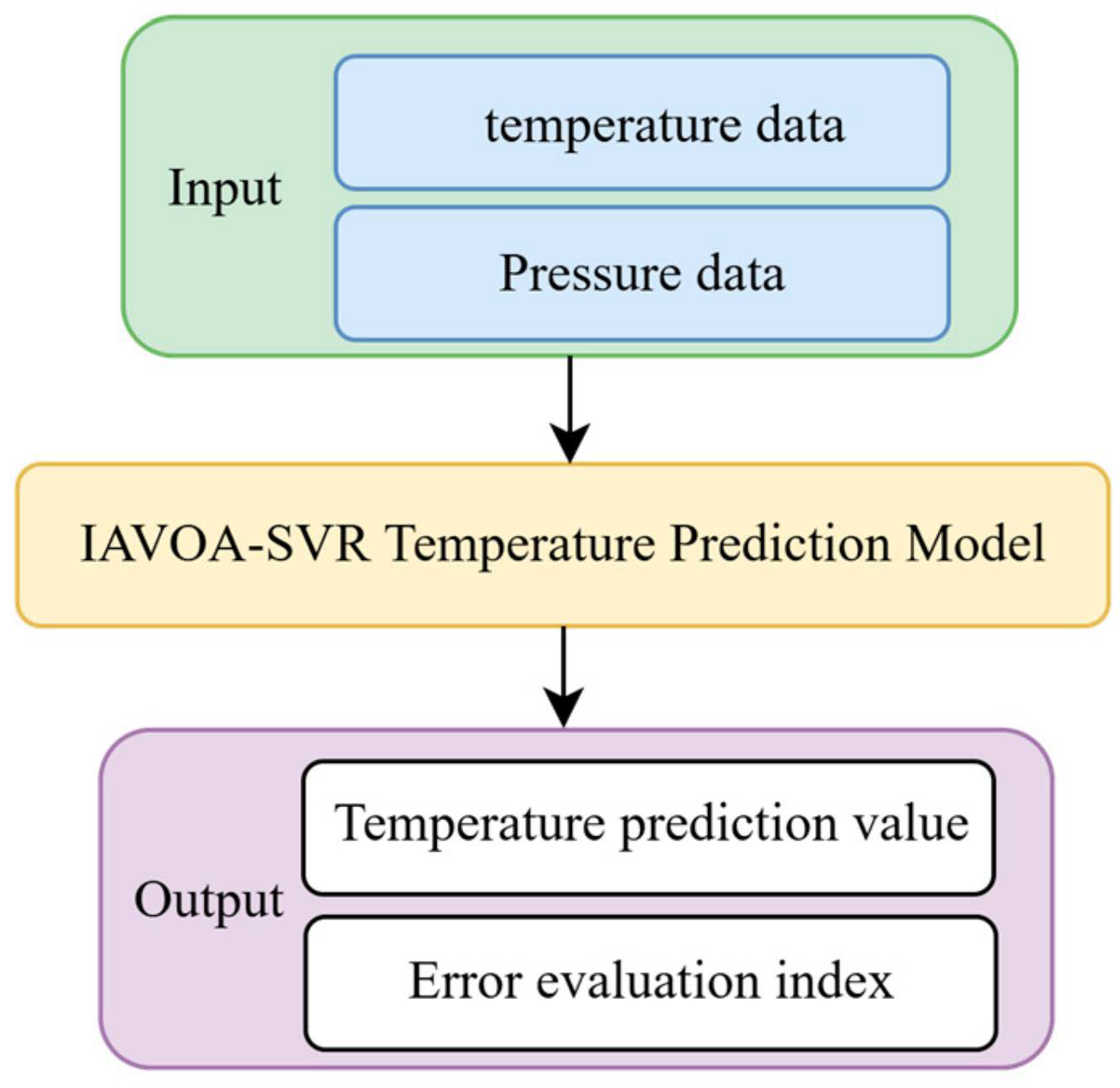
3. Optimized Model for Wind-Tunnel Thermal Prediction

Since its proposal, the AVOA algorithm has attracted the attention of many scholars and has achieved a large number of research results in the fields of new energy, medical and health care and mechanical engineering [22]. This paper innovatively combines AVOA with Support Vector Regression (SVR) and proposes an Improved African Vulture Optimization Algorithm (IAVOA) based on adaptive chaotic mapping and local search enhancement to conduct combined optimization of the parameters in support vector regression, and it shows the optimal prediction accuracy in the temperature prediction of actual wind-tunnel test data. All the experiments were conducted in the MATLAB R2021b environment.

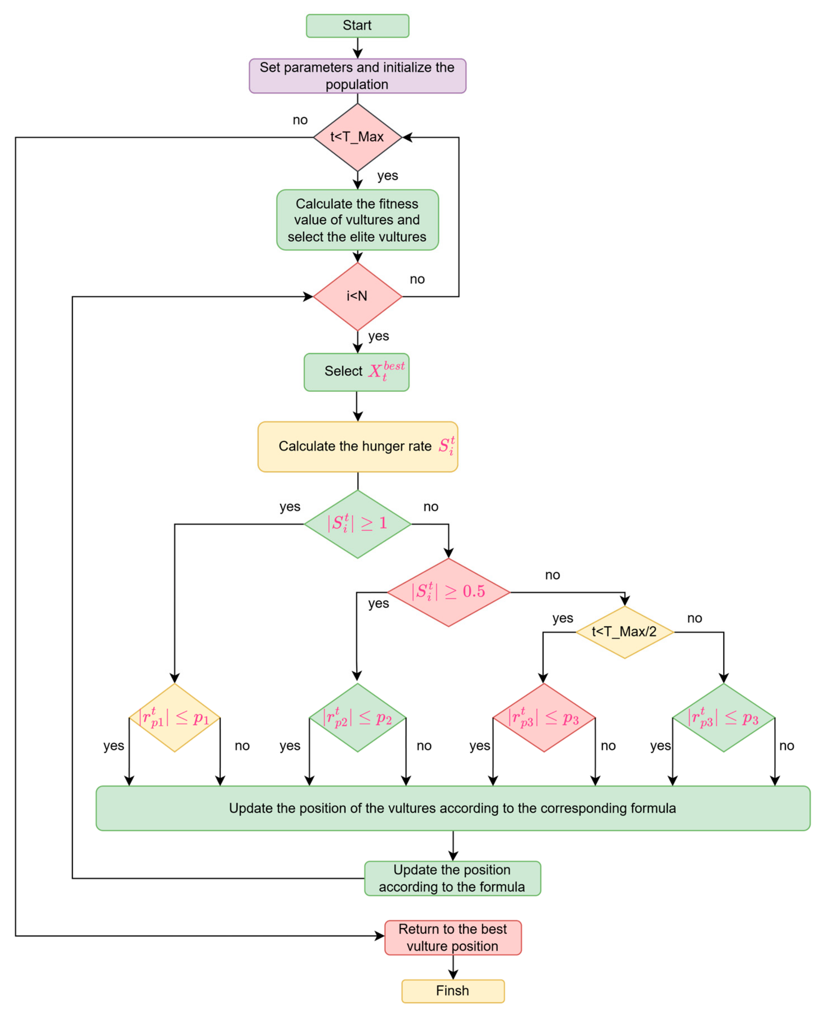
3.1. Improved African Vulture Optimization Algorithm (IAVOA)

(1)

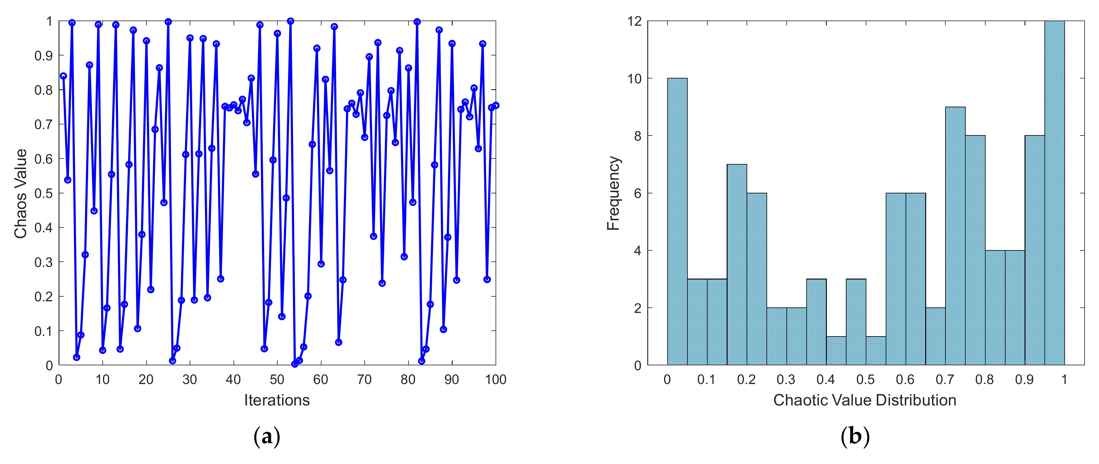
Adaptive chaotic mapping

Based on the problems existing in the traditional basic AVOA, such as being prone to fall into local optimum and the search accuracy needing improvement, this study proposes an Improved African Vulture Optimization Algorithm (IAVOA). This algorithm optimizes the iterative update process of the population by introducing the Adaptive Chaotic Mapping (ACM) mechanism, in order to enhance the diversity and global-search ability of the population. Meanwhile, the Enhanced Local Search (ELS) strategy is adopted to conduct a fine search of the surrounding areas of excellent individuals in the later stage of the algorithm iteration, improving the convergence speed and solution accuracy of the algorithm.

ACM enhances the global-search ability of the algorithm by introducing nonlinear dynamic behavior and avoids falling into local optimum. The random sequence generated by the Logistic chaotic mapping function has the characteristic of distinct elements. This characteristic can effectively solve the problem of uneven initialization distribution of the population. It not only avoids the local optimal trap caused by excessive aggregation of individuals, but also prevents the reduction of search efficiency due to overly dispersed distribution. This unique property significantly enhances the global-exploration ability of the algorithm and provides a more efficient search-space traversal mechanism for the optimization process. The generation of chaotic sequences using Logistic chaotic mapping can be expressed as

$${\gamma }^{t+1}=r\cdot {\gamma }^t\cdot \left(1-{\gamma }^t\right)$$

(23)

Among these terms, $r$ is the model control parameter, and $r=4$ is taken. $t$ represents the current number of iterations and $t=1,2,\dots ,T\_Max$, $T\_Max$ is the maximum number of iterations. ${\gamma }^t$ is a chaotic mapping variable that changes with the number of iterations. The parameters of the chaotic mapping are dynamically adjusted according to the fitness value of the current iteration to enhance the adaptive ability of the algorithm. In the actual application process, the initial chaotic mapping variable parameter was set as ${\gamma }^0=0.7$.

Chaotic sequence values and the distribution histogram of chaotic values are important tools for studying the characteristics of chaotic systems. Figure 1 shows the chaotic sequence values and the distribution histogram of chaotic values of the Logistic map after 100 iterations.

Chaotic systems have a sensitive dependence on initial conditions. The chaotic sequences they generate seem random, but in fact follow certain inherent laws. The distribution histogram can visually display the values of chaotic sequences or the distribution of chaotic values, helping us understand the statistical characteristics of chaotic systems.

When calculating the hunger degree of individual vultures ${\tau }^t$, the adjustment parameter for preventing falling into the local optimal solution was introduced into the chaotic map and changed to an adaptive parameter ${\overline{\tau }}^t$, which can be expressed as

$${\overline{\tau }}^t={\gamma }^t\times U\times \left({\sin }^{\omega }\left({\displaystyle \frac{\pi }{2}}\times {\displaystyle \frac{t}{T}}\right)+\cos \left({\displaystyle \frac{\pi }{2}}\times {\displaystyle \frac{t}{T}}\right)-1\right)$$

(24)

$${\gamma }_i^t=4\times {\gamma }_i^{t-1}\times \left(1-{\gamma }_i^{t-1}\right)$$

(25)

Among these terms, $U$ is a random number uniformly distributed in the interval $[-2,2]$.

When the vulture population had completed all the mining strategies, chaotic disturbances were introduced to the current position of the vultures, and the position update mode was determined through the size relationship of random numbers. When $r_{p_3}^t\le p_3$, upper part of Formula (22) becomes

$$X_i^{t+1}={\displaystyle \frac{M_1+M_2}{2}}+{\gamma }_i^t\times R_i^t\times \left(X_{best}^t-X_i^t\right)$$

(26)

When $r_{p_3}^t>p_3$, lower part of Formula (22) becomes

$$X_i^{t+1}=X_{best}^t-\left|X_{best}^t-X_i^t\right|\times S_i^t\times levy(d)+{\gamma }_i^t\times R_i^t\times \left(X_{best}^t-X_i^t\right)$$

(27)

where $R_i^t$ is a random number and $R_i^t\in \left(0,1\right)$.

At the same time, the upper $u{b}^t$ and lower $l{b}^t$ dynamic boundaries of the vulture position were recorded during each iteration update, represented by $u{b}^t$ and $l{b}^t$, respectively. If the dynamic boundary is exceeded during the update process, bounding processing is carried out, which can be expressed as

$$\left\{\begin{array}{cc}{X}_i^{t+1}=u{b}^t& if\\ X_i^{t+1}=l{b}^t& if\end{array}\right.\begin{array}{c}{X}_i^{t+1}>u{b}^t\\ X_i^{t+1}<l{b}^t\end{array}$$

(28)

(2)

Local search enhancement

In the later stage of the algorithm $T\_Max/2<t<T\_Max$, in order to effectively avoid the predicament where the individual positions of vultures fall into local optimum, a local search-enhancement strategy was introduced. The core of this strategy lies in implementing random perturbation operations on the currently obtained optimal solution. By conducting moderate exploration near the optimal solution, the possible local optimal constraints are broken, thereby improving the accuracy and quality of the solution. During the mining stage, local search focuses on the area around the current optimal solution, conducts fine mining on it, and further optimizes the performance of the solution. By integrating the local search mechanism into both key stages, its advantages can be fully exerted, enhancing the global-search ability and local-development ability of the algorithm, and ensuring that the algorithm can maintain efficient and stable search performance at different stages. Local search can be expressed as

$${\overline{X}}_{best}^t=X_{best}^t+0.1\times R_i^t\left(u{b}^t-l{b}^t\right)$$

(29)

where $R_i^t$ is a random number and $R_i^t\in \left(0,1\right)$.

After introducing the random perturbation mechanism to enhance the local search efficiency, in order to further optimize the convergence and stability of the algorithm, this study implemented the retention strategy of the optimal individual based on the hunger index corresponding to the optimal individual of the vulture. Specifically, during the iterative process of the algorithm, when the local search ability is enhanced through random perturbation, the system will conduct a comprehensive evaluation of the performance of all vulture individuals. The above process can be expressed as

$$\left\{\begin{array}{cc}{\stackrel{⌢}{X}}_{best}^t=X_{best}^t& f(X_{best}^t)<f({\overline{X}}_{best}^t)\\ {\stackrel{⌢}{X}}_{best}^t={\overline{X}}_{best}^t& f(X_{best}^t)\ge f({\overline{X}}_{best}^t)\end{array}\right.$$

(30)

Based on the improved scheme of the African Vulture Optimization Algorithm described in the previous section, in order to clearly illustrate the specific implementation process and logical structure of the algorithm, the corresponding pseudo-code of this improved algorithm is presented, as shown in Algorithm 1. The corresponding flowchart is also provided, as depicted in Figure 2.

Algorithm 1 Improves of the African Vulture Optimization Algorithm

Input: Population size of vultures and the maximum number of iterations T_Max Output: The position and fitness value of the vulture 1: Set parameters and initialize the population 2: While (t < T_Max) do 3:  Calculate the fitness of vultures, select elite vultures, and store the data 4:  Set ${X^t}_{{best}_1}$ as the vulture position (the first best position) 5:  Set ${X^t}_{{best}_2}$ as the vulture position (the second best position) 6:  for (each vaulture) do 7:  Select ${X^t}_{best}$ 8:  Calculate the hunger rate ${S^t}_i$ 9:  if ($\left|{S^t}_i\right|\ge 1$) then 10:    if (${r^t}_{p_1}\le p_1$) then 11:       Update the position of the vultures 12:    else 13:       Update the position of the vultures 14:    end if 15:  else 16:    if ($\left|{S^t}_i\right|<1$) then 17:       if ($\left|{S^t}_i\right|\ge 0.5$) then 18:         if (${r^t}_{p_2}\le p_2$) then 19:           Update the position of the vultures 20:         else 21:           Update the position of the vultures 22:         end if 23:       else 24:         if (${r^t}_{p_3}\le p_3$) then 25:           Update the position of the vultures 26:         else 27:           Update the position of the vultures 28:         end if 29:       end if 30:    end if 31:    Update the position of the vulture according to the formula 32:    t = t + 1 33:    if (t > T_Max/2) then 34:       if (${r^t}_{p_3}\le p_3$) then 35:         Update the positions of the vultures 36:       else 37:         Update the positions of the vultures 38:       end if 39:    end if 40:  end while 41: Return ${X^t}_{best}$

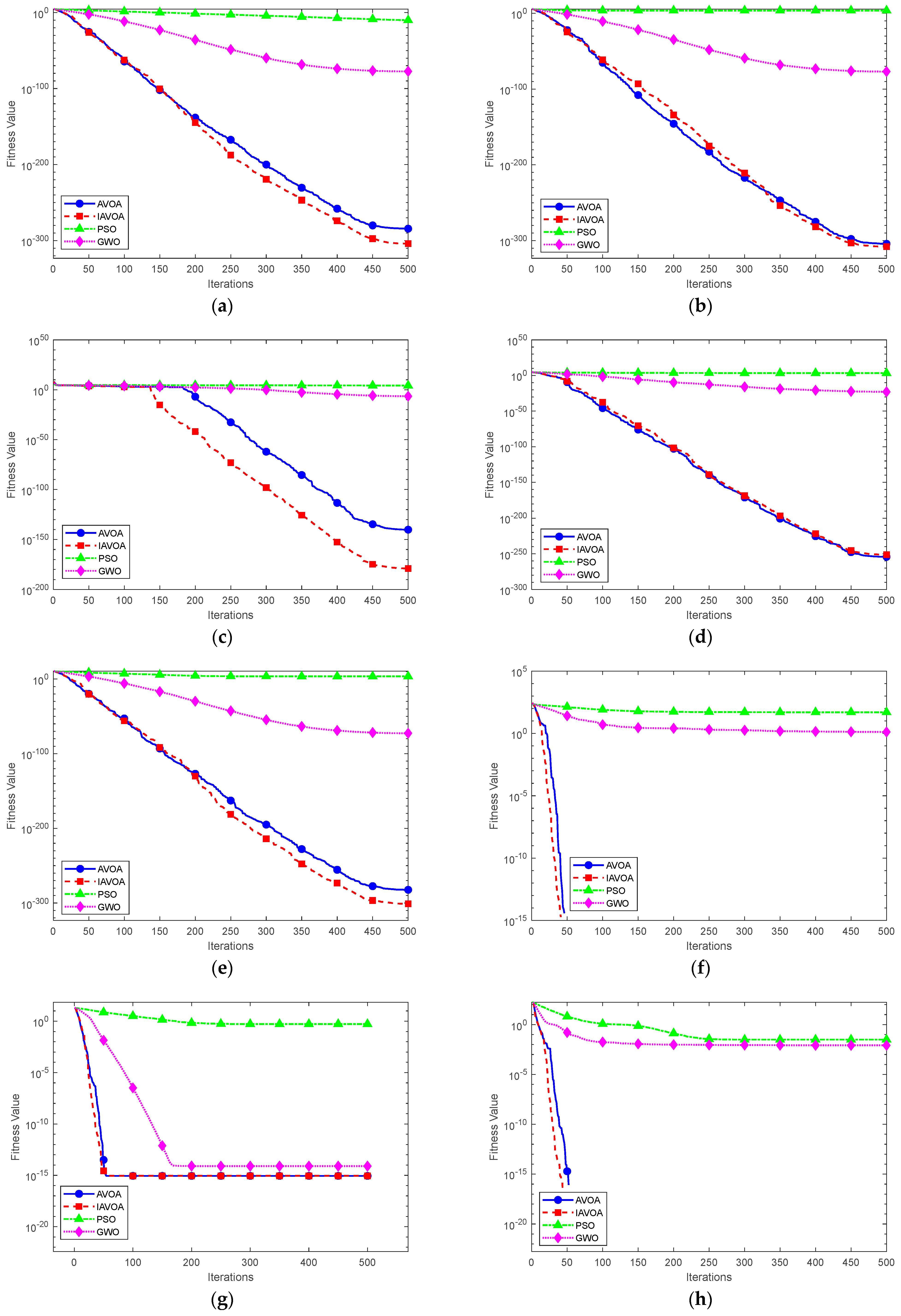
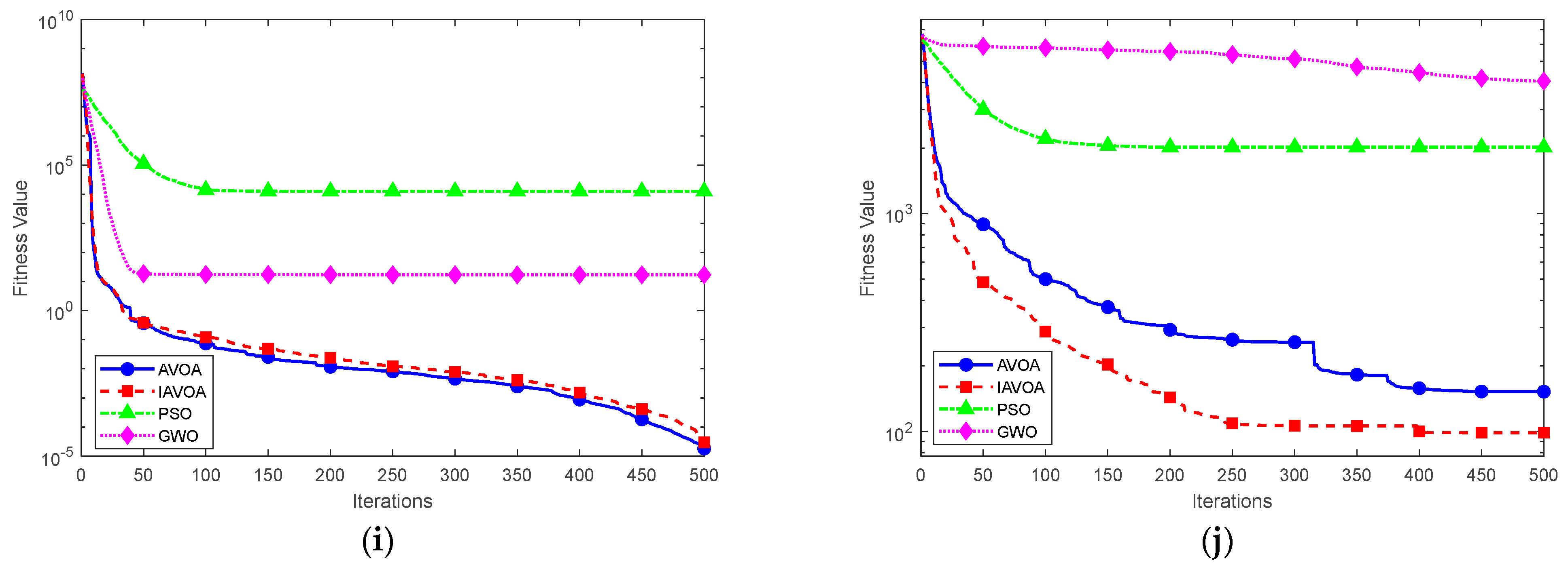
3.2. Benchmark Test Function

This section systematically evaluates the performance of the improved African Vulture Optimization Algorithm (IAVOA) through benchmark function simulation experiments. To verify the effectiveness of the improved algorithm, ten basic test functions with different characteristics were selected. Unimodal functions (Sphere function, Ellipsoid function, Zakharov function, Quadric function, Cigar function) and multimodal functions (Rastrigin function, Ackley function, Griewank function, Rosenbrock function, Schwefel function) were used to evaluate the performance of the IAVOA algorithm, and a comprehensive test was conducted. The benchmark functions are used to test the performance of the optimization functions and to evaluate and compare the advantages of different optimization algorithms. These functions have known optimal solutions and are defined in multi-dimensional spaces to test the global search, local search and function optimization capabilities of the algorithms [23]. The IAVOA algorithm was compared with the basic African Vulture Optimization Algorithm [21], Particle Swarm Optimization Algorithm [24] and Grey Wolf Optimization Algorithm [25]. After each algorithm ran independently 30 times, an analysis and comparison were conducted. During the experiment, the performance indicators, such as the convergence curve and the accuracy of the optimal solution of the algorithm on different test functions, were recorded in detail.

Ten sets of benchmark test functions are presented, as shown in

Table 1. Ten sets of benchmark test functions.

Test Function	Dimensionality	Search Range	Optimum Value
$f_1\left(x\right)={\displaystyle {\sum }_{i=1}^d{x}_i^2}$	20	[−100,100]	0
$f_2\left(x\right)={\displaystyle {\sum }_{i=1}^{d}i\cdot x_i^2}$	20	[−100,100]	0
$f_3\left(x\right)={\displaystyle {\sum }_{i=1}^d{x}_i^2}+{\left({\displaystyle {\sum }_{i=1}^{d}0.5i{x}_i^2}\right)}^2+{\left({\displaystyle {\sum }_{i=1}^{d}0.5i{x}_i^2}\right)}^4$	20	[−10,10]	0
$f_4\left(x\right)={{\displaystyle {\sum }_{i=1}^d\left({\displaystyle {\sum }_{j=1}^i{x}_j}\right)}}^2$	20	[−100,100]	0
$f_5\left(x\right)=x_1^2+{10}^6{\displaystyle {\sum }_{i=2}^d{x}_i^2}$	20	[−100,100]	0
$f_6\left(x\right)=10d+{\displaystyle {\sum }_{i=1}^d\left[x_i^2-10\cos \left(2\pi x_i\right)\right]}$	20	[−5.2,5.2]	0
$f_7\left(x\right)=-20\exp \left(-0.2\sqrt{{\displaystyle \frac{1}{d}}{\displaystyle {\sum }_{i=1}^d{x}_i^2}}\right)-\exp \left({\displaystyle \frac{1}{d}}{\displaystyle {\sum }_{i=1}^d\cos \left(2\pi x_i\right)}\right)$	20	[−32,32]	0
$f_8\left(x\right)={\displaystyle \frac{1}{4000}}{\displaystyle {\sum }_{i=1}^d{x}_i^2}-{\displaystyle {\prod }_{i=1}^d\cos \left(\frac{x_i}{\sqrt{i}}\right)}+1$	20	[−600,600]	0
$f_9\left(x\right)={\displaystyle {\sum }_{i=1}^{d-1}\left[100{\left(x_{i+1}-x_i^2\right)}^2+{\left(1-x_i\right)}^2\right]}$	20	[−30,30]	0
$f_{10}\left(x\right)=418.9829d-{\displaystyle {\sum }_{i=1}^d{x}_i}\sin \left(\sqrt{\left|x_i\right|}\right)$	20	[−500,500]	0

. In the table, the function $f_1$–$f_5$ is a unimodal test function, with only one global optimal solution and no local optimal solution. It is mainly used to test the convergence speed and development capability of the algorithm and to measure the local-development efficiency of the algorithm. The function $f_6$–$f_{10}$ is a multimodal test function, with multiple local optimal solutions, and the global optimal solution is surrounded by local optima. It is used to test the global-search ability and the ability to escape the local optima of the algorithm. To measure the global-exploration ability of the algorithm, these functions are the standard test sets in the field of optimization, which can expose the potential flaws of the algorithm, such as premature convergence and becoming trapped in local optima. The performance of the IAVOA algorithm can be evaluated through the above test functions.

Under the premise of the same environmental configuration, with the aid of the Matlab r2021b numerical computing platform, modeling work was carried out for four optimization algorithms. In terms of specific parameter settings, the population size of the four optimization algorithms was uniformly set at 30, and the maximum number of iterations was set at 500. The settings of other parameters involved in the algorithms are shown in

Table 2. Parameter settings.

Algorithm	Parameter
GWO [25]	$a$: 2 decrease to 0
PSO [24]	$c_1=c_2=1.49$$,\omega =0.8$
AVOA [21]	$p_1=p_2=p_3=0.5$$,\alpha =0.8$$,\beta =0.2$$,\omega =2.5$
IAVOA	$p_1=p_2=p_3=0.5$$,\alpha =0.8$$,\beta =0.2$$,\omega =2.5$

.

The iterative curve of the test function is shown as Figure 3, and the test values of the basic functions are presented in

Table 3. Test values of basic functions.

Basic Function	Algorithm	Mean Value	Standard	Maximum	Minimum
$f_1$	AVOA [21]	2.27 × 10−28	0.00	0.00	2.37 × 10−31
	GWO [25]	1.17 × 10−7	4.06 × 10−7	1.40 × 10−8	2.12 × 10−7
	PSO [24]	4.87 × 10−1	6.18 × 10−1	1.88 × 10−1	3.16 × 10−1
	IAVOA	2.09 × 10−30	0.00	0.00	1.74 × 10−31
$f_2$	AVOA [21]	2.16 × 10−29	0.00	0.00	6.48 × 10−29
	GWO [25]	4.75 × 10−7	9.67 × 10−7	6.30 × 10−8	3.75 × 10−7
	PSO [24]	2.66 × 100	8.27 × 100	3.22 × 10−1	4.00 × 100
	IAVOA	1.45 × 10−31	0.00	0.00	4.36 × 10−30
$f_3$	AVOA [21]	2.80 × 10−16	0.00	3.83 × 10−27	8.41 × 10−16
	GWO [25]	1.97 × 10−1	9.49 × 10−9	3.06 × 10−21	5.21 × 10−8
	PSO [24]	1.72 × 100	9.79 × 103	1.89 × 103	4.69 × 104
	IAVOA	1.38 × 10−19	0.00	3.47 × 10−26	4.15 × 10−18
$f_4$	AVOA [21]	1.53 × 10−23	0.00	4.94 × 10−32	4.60 × 10−23
	GWO [25]	2.69 × 10−2	1.44 × 10−21	6.91 × 10−3	7.93 × 10−2
	PSO [24]	2.01 × 1030	2.80 × 103	9.71 × 10−1	1.01 × 104
	IAVOA	5.18 × 10−24	0.00	5.17 × 10−31	1.54 × 10−24
$f_5$	AVOA [21]	3.49 × 10−30	0.00	0.00	1.04 × 10−30
	GWO [25]	2.92 × 10−7	6.84 × 10−73	1.33 × 10−77	3.10 × 10−7
	PSO [24]	4.00 × 103	4.98 × 103	2.75 × 10−6	1.00 × 104
	IAVOA	1.62 × 10−28	0.00	0.00	4.87 × 10−28
$f_6$	AVOA [21]	0.00	0.00	0.00	0.00
	GWO [25]	9.99 × 10−1	1.78 × 10	0.00	5.94 × 100
	PSO [24]	5.39 × 101	3.65 × 101	2.38 × 101	2.22 × 102
	IAVOA	0.00	0.00	0.00	0.00
$f_7$	AVOA [21]	8.88 × 10−16	0.00	8.88 × 10−16	8.88 × 10−16
	GWO [25]	2.06 × 101	9.89 × 10−2	2.04 × 101	2.08 × 101
	PSO [24]	2.00 × 101	8.96 × 10−2	2.00 × 101	2.04 × 101
	IAVOA	6.88 × 10−16	0.00	8.88 × 10−16	8.88 × 10−16
$f_8$	AVOA [21]	0.00	0.00	0.00	0.000
	GWO [25]	4.71 × 10−3	1.11 × 10−2	0.00	5.15 × 10−2
	PSO [24]	2.14 × 10−2	1.83 × 10−2	4.62 × 10−13	6.14 × 10−2
	IAVOA	0.00	0.00	0.00	0.00
$f_9$	AVOA [21]	1.15 × 10−5	9.55 × 10−6	5.60 × 10−7	3.67 × 10−5
	GWO [25]	1.70 × 101	4.90 × 10−1	1.61 × 101	1.80 × 101
	PSO [24]	3.63 × 103	1.63 × 104	3.61 × 100	9.00 × 104
	IAVOA	2.10 × 10−5	1.76 × 10−5	1.63 × 10−6	6.08 × 10−5
$f_{10}$	AVOA [21]	3.04 × 102	4.81 × 102	2.54 × 10−4	1.81 × 103
	GWO [25]	4.05 × 103	5.65 × 102	3.28 × 103	5.53 × 103
	PSO [24]	2.14 × 103	4.96 × 102	8.30 × 102	3.01 × 103
	IAVOA	1.02 × 102	2.84 × 102	2.54 × 10−4	1.42 × 103

. By comparing and analyzing the average value, standard deviation, maximum value and minimum value of the average results obtained by running each test function independently for 30 times through different algorithms, the performance of different algorithms on various test functions could be intuitively reflected. The research results show that, among the ten test functions, the IAVOA algorithm demonstrated more superior performance compared with the AVOA algorithm, the PSO algorithm and the GWO algorithm.

The experimental results show that, compared with the AVOA algorithm, the PSO algorithm and the GWO algorithm, the IAVOA algorithm achieved better optimization effects on all test functions, significantly improved the convergence speed and effectively enhanced the solution accuracy. This fully proves the effectiveness of introducing adaptive chaotic mapping and enhancing the local search strategy for the performance of the IAVOA algorithm.

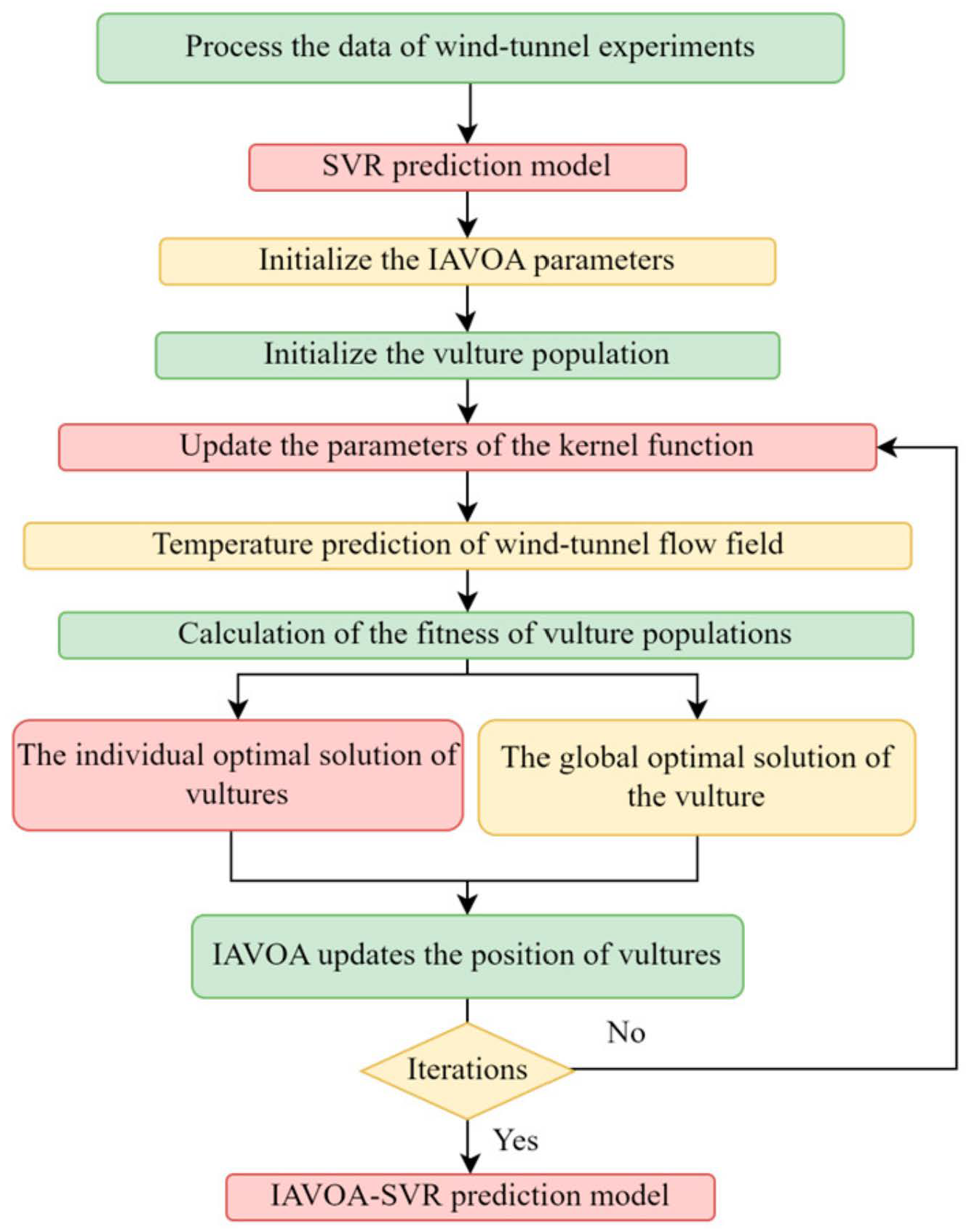
3.3. Improved AVOA-Optimized SVR

Based on the IAVOA algorithm and aiming at the theoretical model of Support Vector Regression (SVR), an improved vulture algorithm was constructed to optimize the support vector regression wind-tunnel temperature prediction model (IAVOA-SVR). During the construction process of the SVR model, the data processed by kernel principal component analysis and phase-space reconstruction was taken as the input set of the model. The ratio of the training set to the test set was 6:4, and the commonly used radial basis kernel function was selected as the kernel function type. The IAVOA algorithm was used to perform parameter-optimization operations on the penalty parameters of SVR, the insensitive loss function and the parameters of the radial-basis kernel function, aiming to obtain a set of optimal parameter combinations. By reasonably adjusting these parameters, the complexity and generalization ability of the model could be effectively controlled, thereby enabling the model to exhibit better performance with different datasets and various tasks. The steps, schematic diagrams and flowcharts of IAVOA-SVR are, respectively, shown in

Table 4. Steps of the IAVOA-SVR algorithm.

Step	Steps of the IAVOA-SVR Algorithm
Step1	Carry out the kernel principal component analysis and phase-space reconstruction processing on the wind-tunnel test data
Step2	Construct the SVR temperature prediction model and take the parameters of SVR to be optimized as the input of IAVOA
Step3	Initialize parameters such as the population size and the number of iterations of IAVOA
Step4	Establish the optimization objective function and take the SVR temperature-training model error as the IAVOA fitness function
Step5	Update the SVR parameters as the number of iterations increases
Step6	Update the record of the optimal-fitness function and the optimal-parameter combination
Step7	Determine whether the end condition (maximum number of iterations) is met. If it is not completed, return to the fifth step
Step8	Output the optimal fitness result and the optimal parameter combination

and Figure 4 and Figure 5.

4. Experimental Results and Analysis

4.1. Data Introduction

The wind-tunnel test data in this paper are derived from two sets of temperature and pressure data collected at the high-altitude wind-tunnel test site of AVIC Aerodynamics Research Institute (Shenyang). The wind-tunnel test data involve two sets of data sample sets of different sizes, with the sample sizes reaching 1600 cases and 2000 cases, respectively. The data dimension covers the key parameter system during the wind-tunnel test process: specifically, it includes the inlet temperature value of the wind-tunnel test section, the average outlet temperature value, the average temperature of the eight independent module areas distributed within the wind-tunnel test section, the medium temperature of the four different functional areas and the inlet pressure-parameter of the entire wind-tunnel-test section. Among the above-mentioned multi-dimensional characteristic parameters, the average outlet temperature was set as the target variable to be predicted for the research.

4.2. Data Preprocessing

For the two groups of wind-tunnel test datasets, based on the theoretical framework of dimensionality reduction of kernel principal component analysis mentioned earlier, the dimensionality reduction processing of multi-dimensional wind-tunnel test datasets was implemented in the Matlab r2021b numerical computing environment. During the dimensionality reduction process, the Gaussian Kernel function was adopted as the nonlinear mapping function, and its kernel width parameter was determined to be $\sigma =0.85$ by using the cross-validation method. Based on the cumulative contribution rate criterion, the principal component screening threshold was set at 95%, that is, the top four principal components were selected so that their cumulative-variance interpretation rate reached more than 95% of the total variance, ensuring that the data after dimensionality reduction could not only effectively retain the original information but also significantly reduce the computational complexity.

Each group of data was divided into the training set and the test set in a ratio of 6:4. To eliminate the influence of dimensions, the experimental data were normalized and the data sizes between were mapped. The phase-space reconstruction was carried out according to the steps mentioned above. In this process, the data were decomposed into 200 disjoint time series, and the embedding dimensions were taken as 2, 3, 4, 5, with the radius $r=j\ast sigma/2$ ($j=1,2,3,4$, $sigma$ is the average value of each column). The verification statistics sequence $\overline{S}(\tau )$, maximum deviation $\Delta \overline{S}(\tau )$ and index curves $S_{cor}(\tau )$ of the wind-tunnel test data after dimension reduction obtained by using the Matlab r2021b platform are shown in Figure 6.

In the training dataset, cross-validation was used to determine the values of the parameters. For data 1, according to the calculation results of Matlab, the $\Delta \overline{S}(\tau )$ first minimum value is 8, the $\Delta \overline{S}(\tau )$ first minimum value taken is taken as the optimal time delay ${\tau }_d=8$ and the $S_{cor}(\tau )$ global minimum value taken is taken as the time window length of the time series ${\tau }_w=190$. According to ${\tau }_w=(m-1){\tau }_d$, $m=22$ is obtained. If it exceeds the set range, the embedding dimension is taken to be $m=5$.

For data 2, according to the calculation results of Matlab, the $\Delta \overline{S}(\tau )$ first minimum value is 7, the $\Delta \overline{S}(\tau )$ first minimum value taken is taken as the optimal time delay ${\tau }_d=7$ and the $S_{cor}(\tau )$ global minimum value taken is taken as the time window length of the time series ${\tau }_w=170$. According to ${\tau }_w=(m-1){\tau }_d$, obtained $m=25$ is obtained. If it exceeds the set range, the embedding dimension is taken as $m=5$.

4.3. Error-Evaluation Index

In the process of conducting a comprehensive and precise assessment of the performance of complex machine-learning models, the scientific and reasonable selection of error-evaluation indicators is a crucial link. These indicators are not only quantitative tools for measuring the superiority or inferiority of the model’s predictive ability, but also important bases for guiding model optimization, parameter tuning and practical application decisions.

(1) The Root Mean Square Error (RMSE) is a common indicator for measuring the difference between the predicted values of the model and the true values. The root mean square error can be expressed as

$$R_M={\left({\displaystyle \frac{1}{M-1}}{\displaystyle \sum _{i=1}^M(p_i-o_i}{)}^2\right)}^{1/2}$$

(31)

Among these terms, $M$ represents the sample size, $p_i$ represents the predicted value and $o_i$ represents the true value. The $R_M$ Range $\left[0,+\infty \right)$, when the predicted value exactly matches the true value, is equal to $0$, that is, the perfect model. The greater the error between the predicted value and the true value, the greater the value;

(2) The Mean Absolute Percentage Error (MAPE) is a statistical indicator used to measure the relative error between the predicted values and the actual values of the prediction model. The mean absolute percentage error can be expressed as

$$M_A={\displaystyle \frac{100\%}{M}}{\displaystyle \sum _{i=1}^M\left|\frac{o_i-p_i}{o_i}\right|}$$

(32)

Among these terms, $M$ represents the sample size, $p_i$ represents the predicted value, $o_i$ represents the true value, the $M_A$ range is $\left[0,+\infty \right)$, $M_A$ is $0$ represents the perfect model and greater than $1$ indicates a poor model. Among multiple prediction models, the lower $M_A$ model usually has better prediction accuracy;

(3) The Normalized Root Mean Square Error (NRMSE) is an indicator used to evaluate the performance of the prediction model. The normalized root mean square error can be expressed as [26]

$$N_R={\left({\displaystyle \frac{{\displaystyle {\sum }_{i=1}^M{\left(p_i-o_i\right)}^2}}{{\displaystyle {\sum }_{i=1}^M{\left(o_i-\overline{o}\right)}^2}}}\right)}^{{\displaystyle \raisebox{1ex}{$1$}\!\left/ \!\raisebox{-1ex}{$2$}\right.}}$$

(33)

Among these terms, $M$ represents the sample size, $p_i$ represents the predicted value, $o_i$ represents the true value and $\overline{o}$ represents the average value of the true value. The $N_R$ value range of is $\left[0,1\right]$;

(4) Mean Absolute Deviation (MAD) is a statistical indicator for measuring the degree of dispersion of a set of data, representing the average value of the absolute deviation of each data point from the data mean. The mean absolute deviation can be expressed as

$$M_D={\displaystyle \frac{1}{M}}{\displaystyle \sum _{i=1}^M\left|o_i-p_i\right|}$$

(34)

Here, $M$ represents the sample size, $p_i$ represents the predicted value and $o_i$ represents the true value, and the mean absolute deviation is a simple extension of the absolute variance. It sums the absolute variance and divides the resulting result by the number of records. The mean absolute deviation is an error statistic value, which calculates the average distance between each pair of actual data points and the fitted data points;

(5) Coefficient of determination ($R^2$) is an indicator for measuring the prediction accuracy of the regression model, and its value range is usually between 0 and 1. The specific formula is as follows:

$$R^2=1-{\displaystyle \frac{{\displaystyle {\sum }_{i=1}^M{\left(o_i-p_i\right)}^2}}{{\displaystyle {\sum }_{i=1}^M{\left(o_i-\overline{o}\right)}^2}}}$$

(35)

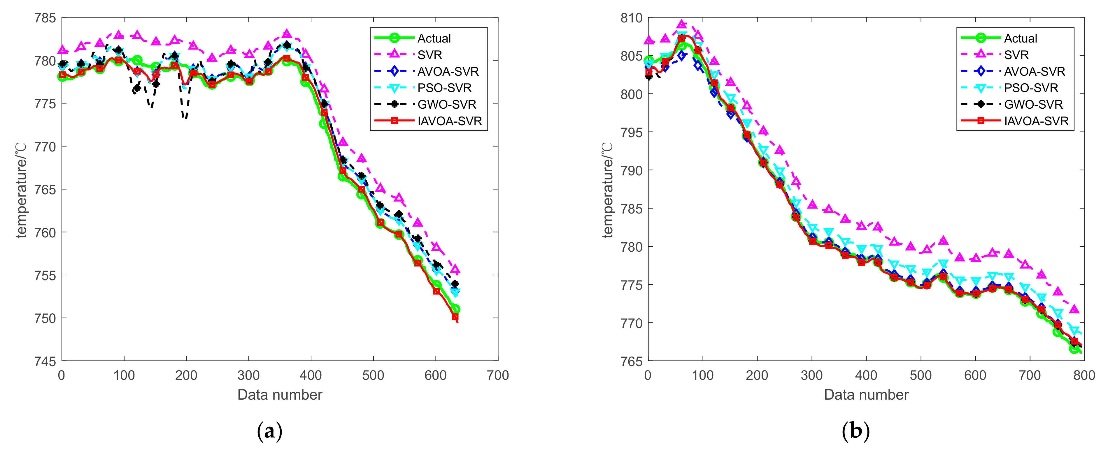
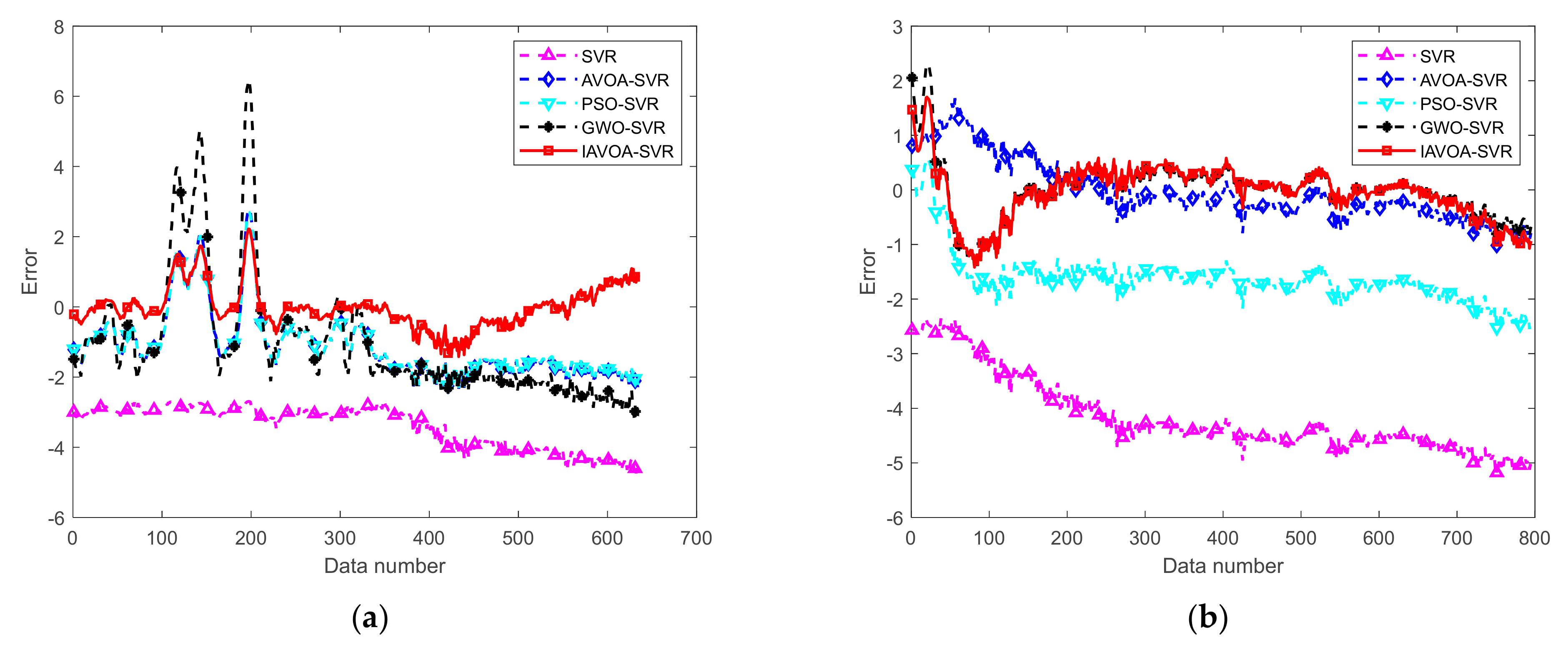
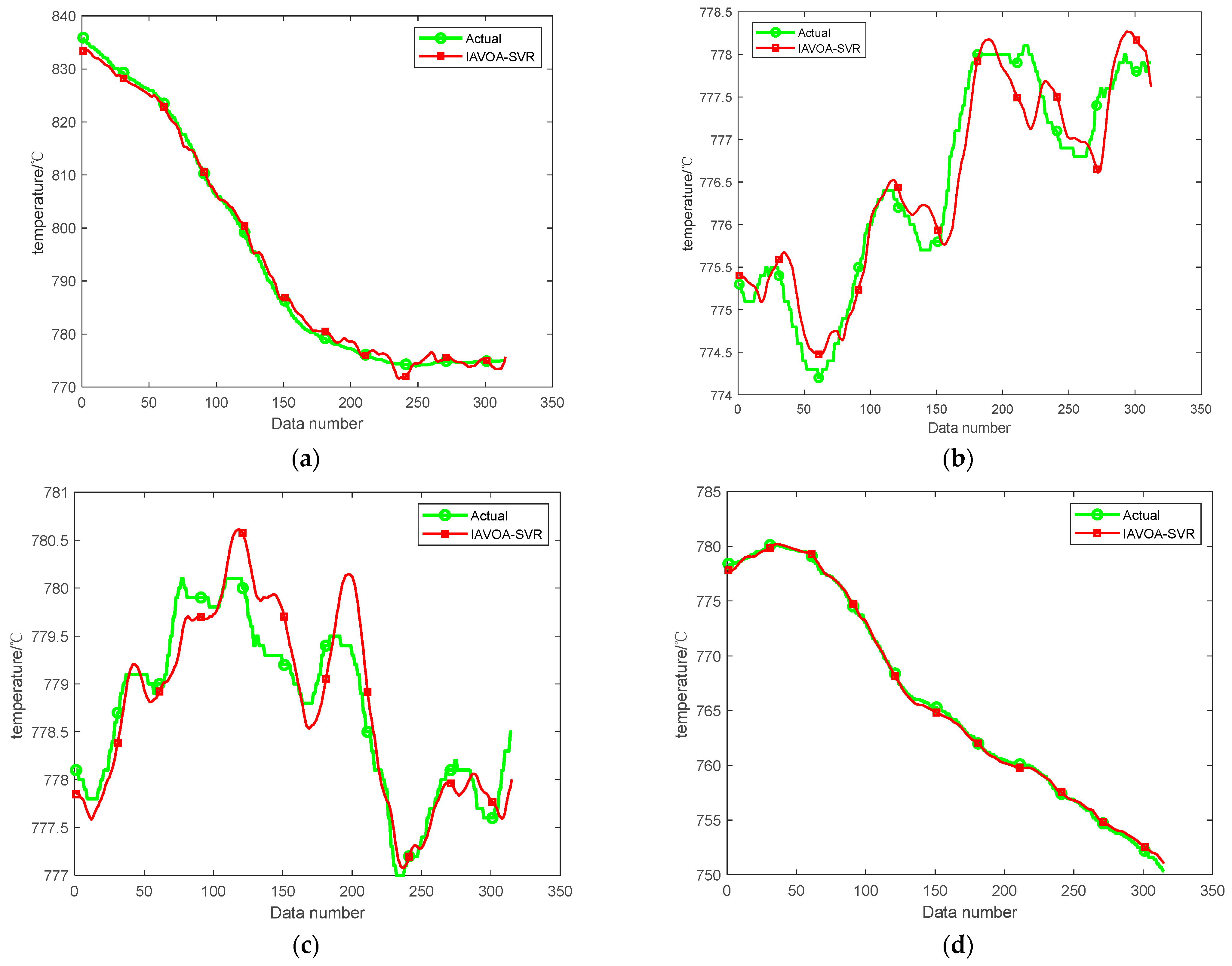
4.4. Actual Wind-Tunnel Data Analysis

A confirmatory analysis experiment was conducted on the IAVOA SVR model proposed in this chapter. The IAVOA SVR model was compared and analyzed with the benchmark SVR model, with the AVOA-SVR model adopting the traditional optimization strategy, the PSO-SVR model based on particle swarm optimization and the GWO-SVR model based on gray Wolf optimization. The optimization algorithm parameters of each comparison model were strictly set in accordance with the parameters shown in Table 2. The wind-tunnel test dataset was divided into the training set and the test set in a ratio of 6:4, and the data were subjected to kernel principal component analysis for dimension reduction and phase-space reconstruction processing. For the parameters $C$, $g$ of the SVR model, the root mean square error between the predicted value and the actual value was taken as the fitness function. All experiments were completed in the Matlab r2021b environment. The error evaluation indicators of each model’s prediction for the two groups of data are shown in

Table 5. Data 1 error evaluation index of different models.

Data 1	SVR [27]	AVOA-SVR [28]	PSO-SVR [29]	GWO-SVR [30]	IAVOA-SVR
$R_M$	3.4530	0.7040	1.8180	1.4427	0.5305
$M_A$	4.40 × 10−3	7.99 × 10−4	0.0016	0.0017	5.91 × 10−4
$N_R$	0.3716	0.0758	0.1956	0.1553	0.0571
$M_D$	3.4027	0.6139	1.259	1.3386	0.4542
$R^2$	0.8618	0.9747	0.9512	0.9757	0.9956

and

Table 6. Data 2 error evaluation index of different models.

Data 2	SVR [27]	AVOA-SVR [28]	PSO-SVR [29]	GWO-SVR [30]	IAVOA-SVR
$R_M$	4.2189	0.8093	2.3603	0.6417	0.5061
$M_A$	0.0053	8.63 × 10−4	0.0030	6.15 × 10−4	4.53 × 10−4
$N_R$	0.3522	0.0676	0.1970	0.0536	0.0422
$M_D$	4.1594	0.6793	2.3247	0.4835	0.3575
$R^2$	0.8759	0.9877	0.9781	0.9800	0.9983

, respectively. The iterative curve of the fitness function is shown in Figure 7. The predicted values and the true values are shown in Figure 8, and the error is shown in Figure 9.

The experimental results demonstrate the effectiveness of the IAVOA algorithm in optimizing the parameters of the Support Vector Regression (SVR) model for wind-tunnel temperature prediction. The convergence speed of the IAVOA algorithm is significantly faster than that of the AVOA, PSO and GWO algorithms. To comprehensively evaluate the prediction performance of the IAVOA-SVR model, we employed various error evaluation metrics, including Root Mean Square Error (RMSE), Mean Absolute Percentage Error (MAPE), Normalized Root Mean Square Error (NRMSE) and Mean Absolute Deviation (MAD). The experimental results show that the IAVOA-SVR model outperforms the AVOA-SVR, PSO-SVR and GWO-SVR models in all error evaluation metrics; the coefficient of determination reached over 0.99, which is the highest among the other models. However, the IAVOA algorithm has certain limitations. In some cases, IAVOA may not always be superior to other algorithms, and its performance can be affected by various factors. It may still encounter difficulties in high-dimensional complex optimization problems. Although IAVOA demonstrates excellent convergence speed and prediction accuracy in optimizing SVR, future research can focus on improving the algorithm structure of IAVOA to enhance its ability to handle high-dimensional problems, thereby expanding its applicability in various fields.

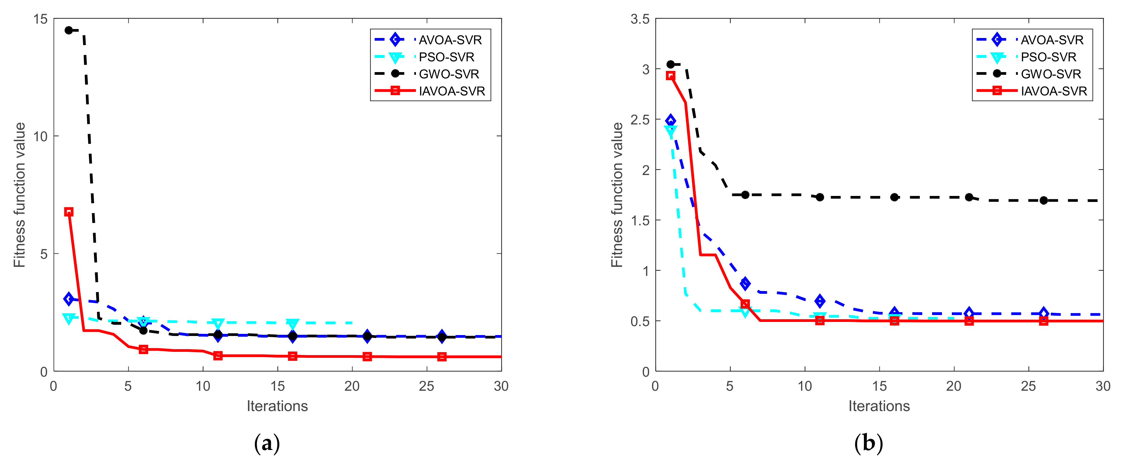
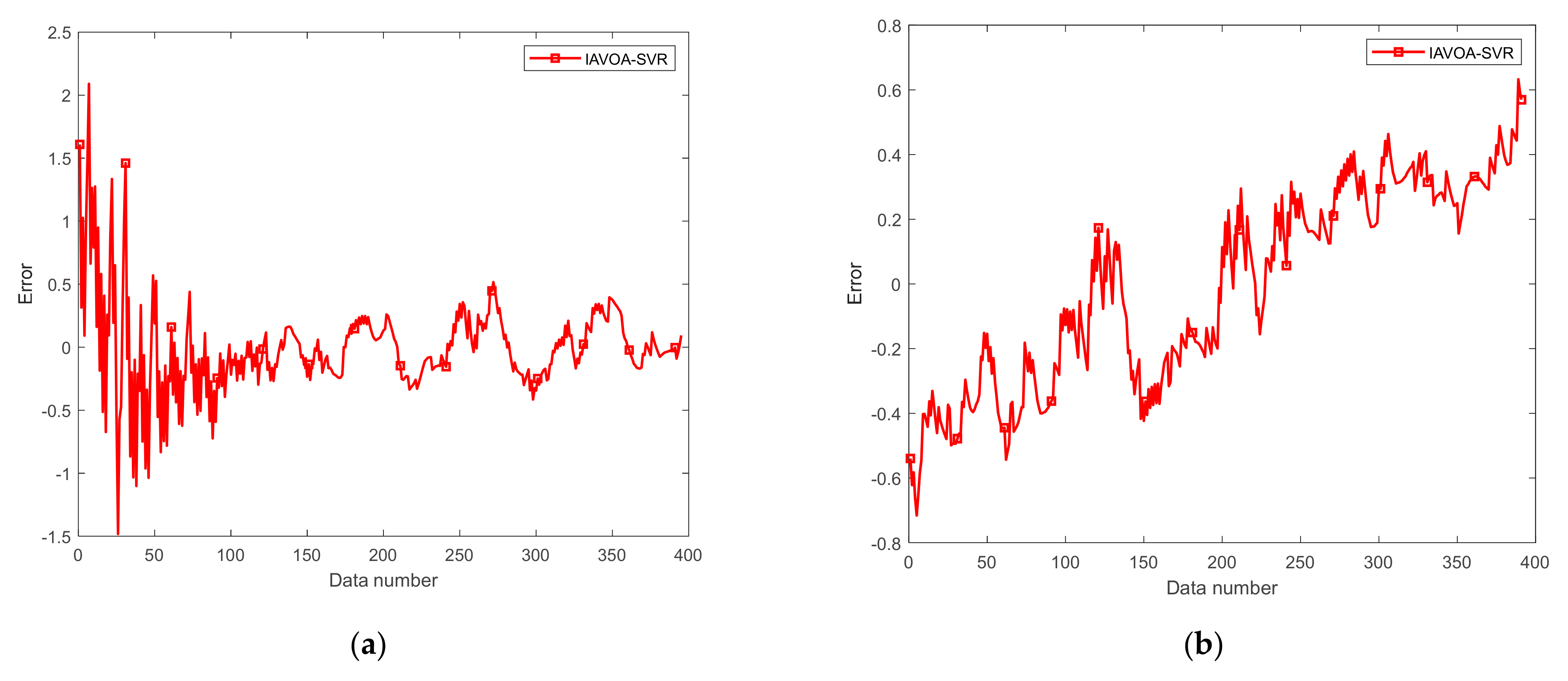
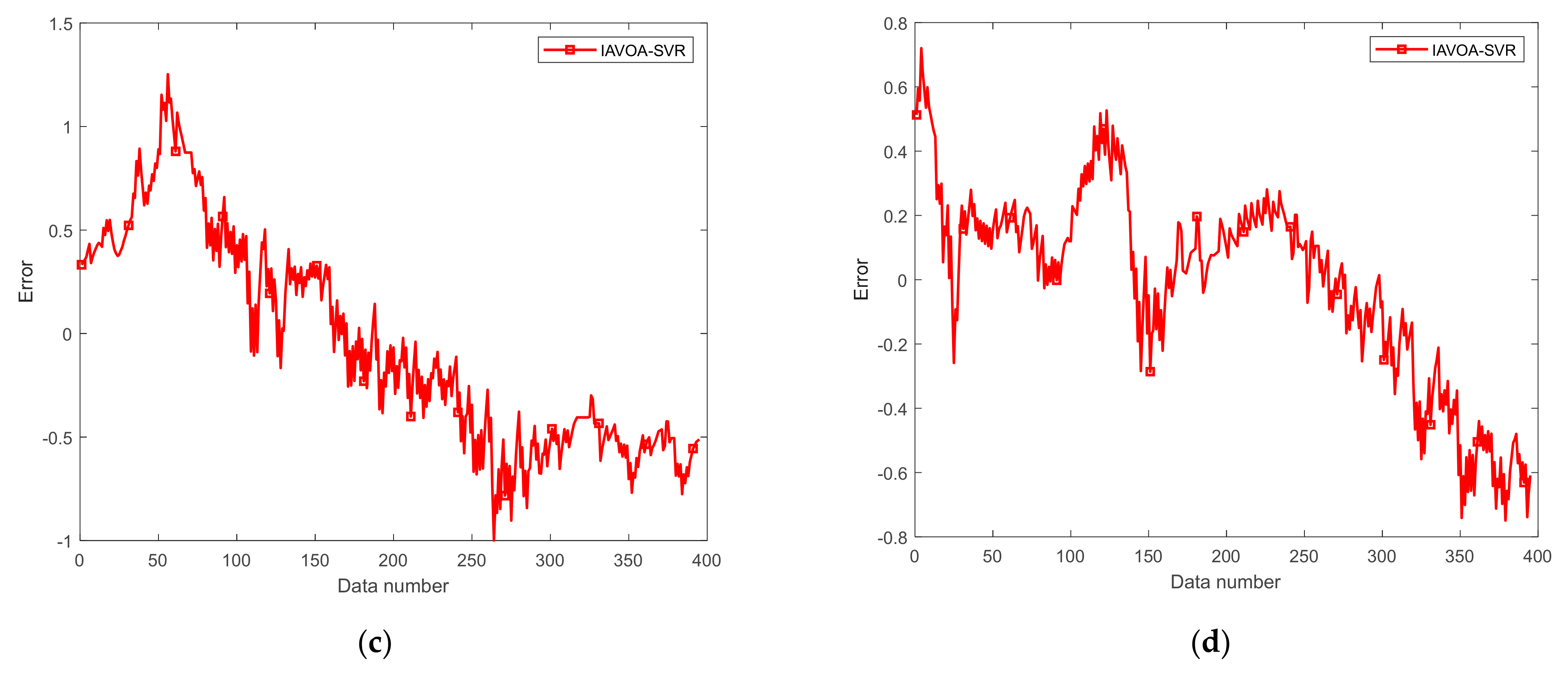
4.5. Validation of the IAVOA-SVR Model

According to the grouping proportions shown in Figure 10, the first group uses 50% for testing and 50% for training. The second group uses 66% for testing and 34% for training. The third group uses 75% for testing and 25% for training. The fourth group uses 80% for testing and 20% for training. The wind-tunnel test data were preprocessed and used as the input of the iva-svr model. Based on the MATLAB r2021b platform, the model of the IAVOA-SVR algorithm was verified. The predicted values and true values of data 1 are shown in Figure 11, the deviations are shown in Figure 12 and the error-evaluation indicators are shown in

Table 7. Data 1 error evaluation index of different data groups.

Data 1	Group 1	Group 2	Group 3	Group 4
$R_M$	1.2778	0.3222	0.2706	0.9739
$M_A$	1.30 × 10−3	3.25 × 10−4	2.77 × 10−4	9.74 × 10−4
$N_R$	0.0587	0.2624	0.3092	0.1018
$M_D$	1.0557	0.2527	2.16 × 10−1	0.7425

. The predicted values and true values of data 2 are shown in Figure 13, the deviations are shown in Figure 14 and the error-evaluation indicators are shown in

Table 8. Data 2 error evaluation index of different data groups.

Data 2	Group 1	Group 2	Group 3	Group 4
$R_M$	0.3764	0.1676	0.5475	0.1535
$M_A$	3.02 × 10−4	1.76 × 10−4	6.07 × 10−4	1.55 × 10−4
$N_R$	0.0344	0.0662	0.0543	0.0519
$M_D$	0.2437	1.41 × 10−1	0.4811	0.1200

.

In Figure 11 and Figure 12, the prediction results from data 1 show that the proposed method can closely approximate the actual temperature values in all four groups. The prediction bias in group 1 is less than 3, while the prediction bias in the other three groups is less than 1, demonstrating good predictive performance. In terms of the prediction results, as shown in Figure 13 and Figure 14, in data 2, the maximum prediction bias is less than 2.5. The prediction results further confirm the proposed method’s ability to predict wind-tunnel test temperature values. Table 7 and Table 8, respectively, calculate the error-evaluation metric values for the proposed method based on four evaluation indicators: $R_M$, $M_A$, $N_R$, and $M_D$, for data 1 and data 2. From the two tables, it can be seen that the proposed method has relatively small error values for all four indicators, demonstrating its prediction stability and effectiveness.

The IAVOA-SVR model established in this chapter has demonstrated outstanding performance in the split and cross-validation of time series. As revealed by splitting and cross-validation analysis of sequence data in different time periods, this model has shown excellent performance. Specifically, satisfactory results have been achieved in the error indicators of root mean square error $R_M$, mean absolute percentage error $M_A$, normalized root mean square error $N_R$ and mean absolute deviation $M_D$. It shows good performance. Based on the above experimental results and in-depth analysis, the effectiveness of the proposed IAVOA-SVR model for temperature prediction of actual wind-tunnel test data has been proved.

5. Conclusions

Based on the actual collected wind-tunnel test data, this paper constructs an intelligent prediction model for the average temperature at the outlet of the wind-tunnel test section. In view of the data characteristics such as nonlinearity, timeliness and chaos existing in the wind-tunnel test data, the KPCA and PSR methods were combined to preprocess the test data. The processed test data provide strong data support for the subsequent construction of the temperature prediction model. However, the traditional wind-tunnel temperature prediction model belongs to the inherent parametric model, which has problems such as insufficient prediction efficiency, accuracy and excessive reliance on human experience. To address this issue, this paper proposes a combination of data-driven intelligent optimization algorithms and machine-learning models to construct the IAVOA-SVR intelligent wind-tunnel temperature prediction model. By aiming to solve problems such as being prone to falling into local optimum and slow convergence speed in traditional AVOA, the structure of AVOA was improved by introducing adaptive chaotic mapping and local search enhancement strategies, and the IAVOA algorithm is proposed. The test experiments of the benchmark functions show that the IAVOA algorithm has a faster iteration speed and better convergence performance. By aiming to solve the problems such as difficult parameter adjustment and the unstable model of SVR, the parameter information of SVR was optimized through IAVOA, and the IAVOA-SVR temperature prediction model was constructed. Comparative analysis was conducted with the common SVR model, PSO-SVR model and GWO-SVR model in two sets of wind-tunnel test data. The results show that in the IAVOA-SVR model proposed in this paper, the root mean square errors of data 1 and data 2 are 0.5305 and 0.5061, respectively, and the determination coefficients are 0.9956 and 0.9983, respectively. This indicates that it has the highest prediction accuracy and the best model error-evaluation indicators. The cross-validation of the time series of the two sets of data indicates the applicability of the IAVOA-SVR model.

In this paper, the African Vulture Optimization Algorithm was improved and optimized through the deep integration of chaos theory and dynamic control strategy. Combined with support vector regression and applied to the actual data prediction of the temperature field in the superb wind tunnel, the research results show that the algorithm proposed in this paper can accurately predict the average temperature at the outlet of the wind-tunnel flow field. The algorithm proposed in this paper has higher prediction accuracy and better error-evaluation indicators compared to the particle swarm algorithm and the grey wolf optimization algorithm, and the proposed temperature prediction model can be combined with the window-sliding mechanism or other theories to construct an online learning model with subsequent development. This not only solves the control problem of the temperature field in the wind tunnel; it also provides an effective solution for the intelligent optimization of complex engineering systems.

References

1. Yule, G.U. On a Method of Investigating Periodicities in Distributed Series, with special reference to Wolfer’s Sunspot Numbers. Phil. Trans. R. Soc. Lond. A 1927, 226, 267–298. [Google Scholar]
2. Winters, P.R. Forecasting sales by exponentially weighted moving averages. Manag. Sci. 1960, 6, 324–342. [Google Scholar]
3. Tsay, R.S. Testing and modeling threshold autoregressive processes. J. Am. Stat. Assoc. 1989, 84, 231–240. [Google Scholar]
4. Jones, S.; Poongodi, S.; Binu, L. Stabilizing controller using backstepping for steady mass flow in a wind tunnel. In Proceedings of the IEEE Recent Advances in Intelligent Computational Systems, Trivandrum, India, 22–24 September 2011; pp. 735–740. [Google Scholar]
5. Castán-Lascorz, M.A.; Jiménez-Herrera, P.; Troncoso, A.; Asencio-Cortés, G. A new hybrid method for predicting univariate and multivariate time series based on pattern forecasting. Inf. Sci. 2022, 586, 611–627. [Google Scholar]
6. Zhang, X.; Zhang, P.; Peng, B.; Xian, Y. Prediction of icing wind tunnel temperature field with machine learning. J. Exp. Fluid Mech. 2022, 36, 8–15. [Google Scholar]
7. Gad, A.G. Particle swarm optimization algorithm and its applications: A systematic review. Arch. Comput. Methods Eng. 2022, 29, 2531–2561. [Google Scholar]
8. Abualigah, L.; Diabat, A.; Mirjalili, S.; Abd Elaziz, M.; Gandomi, A.H. The arithmetic optimization algorithm. Comput. Methods Appl. Mech. Eng. 2021, 376, 113609. [Google Scholar] [CrossRef]
9. Lambora, A.; Gupta, K.; Chopra, K. Genetic algorithm-A literature review. In Proceedings of the 2019 International Conference on Machine Learning, Big Data, Cloud and Parallel Computing, Faridabad, India, 14–16 February 2019; pp. 380–384. [Google Scholar]
10. Price, K.V. Differential evolution. In Handbook of Optimization: From Classical to Modern Approach; Springer: Berlin/Heidelberg, Germany, 2013; pp. 187–214. [Google Scholar]
11. Hansen, N.; Arnold, D.V.; Auger, A. Evolution strategies. In Springer Handbook of Computational Intelligence; Springer: Berlin/Heidelberg, Germany, 2015; pp. 871–898. [Google Scholar]
12. Dorigo, M.; Stützle, T. Ant colony optimization: Overview and recent advances. In Handbook of Metaheuristics; Springer: Berlin/Heidelberg, Germany, 2018; pp. 311–351. [Google Scholar]
13. Jain, N.K.; Nangia, U.; Jain, J. A review of particle swarm optimization. J. Inst. Eng. Ser. B 2018, 99, 407–411. [Google Scholar] [CrossRef]
14. Kıran, M.S.; Fındık, O. A directed artificial bee colony algorithm. Appl. Soft Comput. 2015, 26, 454–462. [Google Scholar] [CrossRef]
15. Zhu, Q.; Zhu, M.; Cui, Q.; Wang, J.; Gu, Z. Research on Partial Discharge Pattern Recognition of Transformer Bushings Based on KPCA and GTO-SVM Algorithm. In Proceedings of the 6th International Conference on Power and Energy Technology, Beijing, China, 12–15 July 2024. [Google Scholar]
16. Li, W.; Yue, H.; Valle-Cervantes, S.; Qin, S.J. Recursive PCA for adaptive process monitoring. J. Process Control 2000, 10, 471–486. [Google Scholar] [CrossRef]
17. Yuan, G.; Ma, Y.; Tan, F.; Zhang, Z. Research on Transformer Fault Diagnosis Based on Improved INGO Optimization LSSVM. In Proceedings of the International Conference on Electrical Engineering and Control Science, Hangzhou, China, 29–31 December 2023. [Google Scholar]
18. Zhou, Z. Machine Learning; Tsinghua University Press: Beijing, China, 2016; pp. 125–128. [Google Scholar]
19. Vapnik, V.N. Pattern recognition using generalized portrait method. Autom. Remote Control 1963, 24, 774–780. [Google Scholar]
20. Mousaei, A.; Naderi, Y.; Bayram, I.S. Advancing State of Charge Management in Electric Vehicles with Machine Learning: A Technological Review. IEEE Access 2024, 12, 43255–43283. [Google Scholar] [CrossRef]
21. Abdollahzadeh, B.; Gharehchopogh, F.S.; Mirjalili, S. African vultures optimization algorithm A new nature-inspired metaheuristic algorithm for global optimization problems. Comput. Ind. Eng. 2021, 58, 107–408. [Google Scholar] [CrossRef]
22. Kumar, C.; Mary, D.M. Parameter estimation of three diode solar photovoltaic model using an Improved African Vultures optimization algorithm with Newton-Raphson method. J. Comput. Electron. 2021, 20, 2563–2593. [Google Scholar] [CrossRef]
23. Kuang, X.; Hou, J.; Liu, X.; Lin, C.; Wang, Z.; Wang, T. Improved African Vulture Optimization Algorithm Based on Random Opposition-Based Learning Strategy. Electronics 2024, 13, 3329. [Google Scholar] [CrossRef]
24. Nebro, A.J.; Durillo, J.; Garcia-Nieto, J.; Coello Coello, C.A.; Luna, F.; Alba, E. SMPSO: Anew PSO-Based Metaheuristic for Multi-Objective Optimization. In Proceedings of the IEEE Symposium on Computational Intelligence in Multicriteria Decision Making, Nashville, TN, USA, 30 March–2 April 2009; pp. 66–73. [Google Scholar]
25. Mirjalili, S.; Mirjalili, S.M.; Lewis, A. Grey wolf optimizer. Adv. Eng. Softw. 2014, 69, 46–61. [Google Scholar] [CrossRef]
26. Mousaei, A.; Naderi, Y. Predicting Optimal Placement of Electric Vehicle Charge Stations Using Machine Learning: A Case Study in Glasgow. In Proceedings of the Iranian Conference on Renewable Energies and Distributed Generation, Qom, Iran, 26 February 2025; Volume 14, pp. 1–7. [Google Scholar]
27. Gao, C.; Ji, W.; Wang, J.; Zhu, X.; Liu, C.; Yin, Z.; Huang, P.; Yu, L. Real-Time prediction of pool fire burning rates under complex heat transfer effects influenced by ullage height: A comparative study of BPNN and SVR. Therm. Sci. Eng. Prog. 2024, 56, 103060. [Google Scholar] [CrossRef]
28. Chen, Z.; Mu, H.; Liao, X.; Ouyang, H.; Huang, D.; Lu, J.; Chen, D. Multiobjective Optimization of the Difficult-to-Machine Material TC18 Based on AVOA-SVR and MOAVOA. JOM 2025, 77, 1727–1745. [Google Scholar] [CrossRef]
29. Zhou, H.; Zhu, J.; Liu, Y. Transformer oil temperature prediction based on PSO-SVR. In Proceedings of the IEEE International Conference on Civil Aviation Safety and Information Technology, Hangzhou, China, 23–25 October 2024; pp. 1286–1290. [Google Scholar]
30. Jin, H.; Hu, Y.; Ge, H.; Hao, Z.; Zeng, Z.; Tang, Z. Remaining useful life prediction for lithium-ion batteries based on an improved GWO–SVR algorithm. Chin. J. Eng. 2024, 46, 514–524. [Google Scholar]
Figure 1. Logistic mapping (a) chaotic sequence of Logistic mapping; (b) chaotic value distribution.
Processes 13 01956 g001
Figure 2. The flowchart of the improved optimization algorithm for African vultures.
Processes 13 01956 g002
Figure 3. Test the iterative curve of the function. (aj) is f 1 f 10 .
Processes 13 01956 g003aProcesses 13 01956 g003b
Figure 4. IAVOA-SVR schematic diagrams chart.
Processes 13 01956 g004
Figure 5. IAVOA-SVR flow chart.
Processes 13 01956 g005
Figure 6. Phase-space reconstruction index (a) data 1; (b) data 2.
Processes 13 01956 g006
Figure 7. Fitness function iteration curve (a) data 1; (b) data 2.
Processes 13 01956 g007
Figure 8. Predicted and actual values (a) data 1; (b) data 2.
Processes 13 01956 g008
Figure 9. Deviation (a) data 1; (b) data 2.
Processes 13 01956 g009
Figure 10. Model validation data set partitioning (a) data 1; (b) data 2.
Processes 13 01956 g010
Figure 11. True and predicted value of data 1 (a) Group 1; (b) Group 2; (c) Group 3; (d) Group 4.
Processes 13 01956 g011
Figure 12. Deviation of data 1 (a) Group 1; (b) Group 2; (c) Group 3; (d) Group 4.
Processes 13 01956 g012
Figure 13. True and predicted value of data 2 (a) Group 1; (b) Group 2; (c) Group 3; (d) Group 4.
Processes 13 01956 g013
Figure 14. Deviation of data 2 (a) Group 1; (b) Group 2; (c) Group 3; (d) Group 4.
Processes 13 01956 g014aProcesses 13 01956 g014b