A Two-Stage Multi-Objective Evolutionary Algorithm for the Dual-Resource Constrained Flexible Job Shop Scheduling Problem with Variable Sublots

Abstract

The dual-resource constrained flexible job shop scheduling problem with variable sublots (DRCFJSP-VS) can be decomposed into four subproblems: the sublot splitting subproblem, the sublot sequencing subproblem, the machine assignment subproblem, and the worker assignment subproblem, which are difficult to solve efficiently using conventional methods. The introduction of variable-size batch splitting and the constraints of multiple levels and skills of workers further increase the complexity of the problem, making it difficult to solve efficiently using conventional methods. This paper proposes a mixed-integer linear programming (MILP) model to solve this complex problem and introduces a two-stage multi-objective evolutionary algorithm (TSMOEA). In the first stage of the algorithm, an improved multi-objective discrete difference evolutionary algorithm is used to optimize the dual-resource constrained flexible job shop scheduling problem; in the second stage, an adaptive simulated annealing algorithm is used to search for variable-size batch splitting strategies. To validate the feasibility of the model, the solution results are obtained using the CPLEX solver and compared with the results of TSMOEA. The performance of TSMOEA is compared with NSGA-II, PSO, DGWO, and WOA on improved instances. The results show that TSMOEA outperforms the other algorithms in both IGD and HV metrics, demonstrating its superior solution quality and robustness.

1. Introduction

In the flexible job shop scheduling problem (FJSP), each operation of a job can be assigned to a different machine, and the processing time on each machine is not necessarily the same [1]. This flexibility allows companies to respond quickly to order changes, adjust production processes, and adapt better to market demand fluctuations. In most large-scale manufacturing enterprises, the production process necessitates dividing orders into multiple sublots for production. Effective batching strategies optimize resource utilization, reduce production time, and ensure timely product delivery. Additionally, skilled workers are crucial for handling complex tasks and ensuring product quality.

Batch splitting scheduling involves dividing workpieces into sublots and scheduling the most appropriate machines for each sublot [2]. Based on the number and size of sublots, batch splitting scheduling can be divided into three categories: equal-sized, consistent-sized, and variable-sized batch splitting. In equal-sized batch splitting, each job has the same number of sublots. In consistent-sized batch splitting, the number of sublots for different jobs may vary, but each type of job maintains consistency in every operation. In variable-sized batch splitting, the number and size of sublots can differ for each operation [3]. This strategy involves a unique batch splitting scheme for each job operation, resulting in a larger search space and increased complexity in solving the scheduling problem. However, compared to equal-sized and consistent-sized strategies, variable-sized batch splitting is better at enhancing machine utilization and processing efficiency due to its flexible sublot division.

In actual production, sublot number and size are constrained by both machine and human resources. If sublots are too large, it leads to excessive working hours for some machines and workers, affecting overall efficiency. If sublots are too small, they must be frequently shifted between workers and machines, making management difficult. A reasonable batch size enhances processing efficiency and distributes workload, thereby reducing worker fatigue. This paper introduces human resource constraints into the production scheduling problem based on variable batch splitting, necessitating the consideration of human resource allocation and efficiency in scheduling optimization when applying the batching strategy.

The remainder of the paper is organized as follows: Section 2 reviews the pertinent literature and summarizes work related to this research. Section 3 details the problem studied, outlines assumptions, and develops a mathematical model. Section 4 introduces a novel two-stage multi-objective evolutionary algorithm that partitions the four subproblems into two parts for independent solving. Section 5 presents experiments conducted for the problem model and compares the proposed algorithm’s results with other algorithms. Section 6 provides a summary and outlook.

2. Literature Review

The flexible job shop scheduling problem (FJSP), introduced by Brucker and Schlie in 1990 [4], has gained significant attention in academic and industrial circles. Swarm Intelligence (SI) and Evolutionary Algorithms (EA) are widely applied in this field [5].

Batch splitting scheduling has gained significant interest in flexible job shop scheduling. Initial studies focused on equal-sized batch splitting in flow shops. Yoon et al. [6] proposed a hybrid genetic algorithm integrating linear programming and pairwise swapping, assuming equal-sized sublots and an infinite-capacity buffer. Chao et al. [7] combined a moving algorithm, net gain, and discrete particle swarm to minimize the total weighted advance and delay objectives. Ventura et al. [8] addressed the finite buffer flow shop problem with blocking using a novel genetic algorithm. Recent advancements include enhancements to algorithms like ant colony optimization [9] and grey wolf optimization [10], all focusing on improving scheduling efficiency in job shop environments.

Consistent-sized batch splitting, which is more aligned with actual production than equal-sized batch splitting, has become the focus of recent research. Zhang et al. [11] Developed a mixed-integer linear programming model and a collaborative variable neighborhood descent algorithm. Wang et al. [12] introduced green scheduling and a multi-objective optimization model to minimize completion time and energy consumption using a multi-objective discrete artificial bee colony algorithm. In flexible job shops, Li et al. [13] proposed a hybrid algorithm combining reinforcement learning and an artificial bee colony algorithm for optimal sublot splitting, thereby reducing maximum completion time. Li et al. [14] developed a mixed-integer planning model for a flexible assembly job shop with batch splitting using a new bionic algorithm based on the artificial bee colony. Pinar et al. [15] proposed a constrained planning model incorporating iterative improvement and large-neighborhood search strategies.

Research on variable-sized batch splitting has increased recently. Wang et al. [16] proposed a two-stage discrete water wave optimization algorithm for a flow shop production system to minimize completion time, with two-wave parallel coding for split and sequential waves. Li et al. [17] developed a decomposition-based multi-objective evolutionary algorithm for hybrid flow shop scheduling, minimizing average dwell time, final stage energy consumption, and early/late arrival values, with novel mutation, crossover, right-shift strategies, and population initialization. Sanchit et al. [18] developed a fast linear search algorithm and a branch-and-bound heuristic method for the 1 + m hybrid flow shop problem. Bozek et al. [19] proposed a two-stage optimization method for flexible job shop scheduling with variable-sized batches. Fatemeh et al. [20] developed a mixed-integer linear programming model and variable neighborhood search algorithms for parallel assembly phases. Li [21] proposed a mixed-integer linear programming model and a hyper-heuristic improved genetic algorithm for flexible job shop scheduling with variable-sized splitting, considering constraints like lead time and changeover time. Li et al. [22] addressed a multi-objective optimization problem considering completion time and total energy consumption using a two-stage multi-objective hybrid algorithm.

Most contemporary manufacturing systems study single resource constraints. However, real production requires considering both machine and human resource constraints. Machines need workers to operate them, and workers have varying skills and efficiencies. These complex workshops with machine and human resource constraints are known as dual-resource constrained (DRC) job shops [23]. Tao et al. [24] proposed an adaptive artificial bee colony algorithm for the distributed hybrid flow shop scheduling problem with resource constraints, aiming to minimize completion time. They also studied adaptive perturbation structure and key plant-based local search. He et al. [25] developed a model for the DRC flexible job shop scheduling problem and an improved African vulture optimization algorithm to optimize completion time and total delay. Gao et al. [26] proposed a mixed-wash multiswarm micro-migratory bird optimization algorithm for the multi-resource constrained flexible job shop scheduling problem, generating multiple micro-clusters at initialization. Each micro-cluster periodically invokes a stochastic mix-and-shuffle process. Additionally, a diversification control strategy based on life aging is proposed to achieve population diversification. Recent studies have focused on dual- or multiple-resource scheduling problems, emphasizing workers’ abilities and skills. Liu et al. [27] addressed the complex product assembly line scheduling problem with multi-skilled worker assignment and parallel team scheduling, optimizing for maximum completion time and team workload imbalance. They proposed an integer planning model and a hybrid coding method for worker assignment and task ordering, along with three improvement strategies based on multi-objective evolutionary algorithms. Liu et al. [28] also considered a hybrid flow shop scheduling problem with multi-skilled workers and fatigue factors by establishing an agent-based simulation system to handle uncertainty in the worker fatigue model. They proposed a novel simulation-based optimization framework combining genetic algorithms and reinforcement learning algorithms. Du et al. [29] addressed the flexible flow shop scheduling problem with dual-resource constraints, considering machines and heterogeneous workers with different skills and capabilities. Their integer planning model allows for the rational assignment of workers to satisfy fatigue constraints using a genetic algorithm with two novel heuristic decoding methods. Peng et al. [30] constructed a model for the multi-objective flexible job shop scheduling problem, considering job transportation time, learning effect constraints, and worker efficiency in operating different machines. They developed a hybrid discrete multi-objective imperial competitive algorithm to minimize processing time, energy consumption, and noise.

Currently, there is limited research on batch splitting scheduling in flexible job shops, with most studies focused on job shops, parallel machine shops, and assembly line job shops. Variable-sized batch splitting is more complex than equal-sized and consistent-sized batch splitting, leading to gradual increases in research on variable-sized batch splitting in recent years. Additionally, studies considering workers’ skills and proficiency in flexible job shops remain limited, and few have explored integrating this aspect into batch splitting scheduling research. The flexible job shop variable-sized batch splitting scheduling problem is a highly complex NP-hard problem. Introducing multi-skill and multi-level constraints on workers significantly increases its space and time complexities, making it challenging to model and solve. In this paper, we develop a mixed-integer linear programming model, dividing the problem into four subproblems: sublot splitting, sublot sorting, machine selection, and worker assignment. These subproblems are addressed in two stages. In the first stage, a two-stage multi-objective evolutionary algorithm is proposed to solve sublot sorting, machine selection, and worker allocation. In the second stage, the optimal batch division scheme is optimized and solved.

3. Problem Description and Formulation

3.1. Problem Description

The dual-resource constrained flexible job shop scheduling problem with variable sublots (DRCFJSP-VS) can be described as follows: There are N types of jobs to be processed, and each job, i, has an original lot size, P_i, and requires O_i operations to be completed. There are M machines available in the job shop for processing the jobs and W workers available for selection. The operations for each job type are predetermined and do not change during the machining process. Each operation can be processed by several different machines in the machine set, and each machine can process various operations. When different machines are selected for an operation, the corresponding machining times vary. Each machine in the job shop must be assigned a worker for operation. Workers have different skills and proficiencies in operating various machines. During the processing of each operation, jobs can be divided into BN_i sublots of varying sizes. The batch splitting scheme does not need to be the same for different operations of the same job. The scheduling objective is to arrange an appropriate batch splitting scheme for each operation of each job and to determine the sequence of different jobs within each sublot to optimize certain indicators.

Additionally, the assumptions of DRCFJSP-VS are as follows:

• All machines and workers are operational at time 0.
• At the same time, a worker can operate only one machine, and a machine can be operated by only one worker.
• At the same time, a machine can process only one operation.
• Once an operation has started, no interruption is allowed. When a machine starts processing a sublot of a certain operation, it must complete the current sublot before processing the next. Workers can also be transferred between machines after completing the sublot.
• There is no sequence of operations between sublots of different jobs. Therefore, sublots of different operations of different jobs can be mixed.
• A sequence of operations is required within a sublot of a given job type. The next operation of the sublot cannot commence until all previous operations are completed.
• The total size of sublots for each operation must be equal to the original lot size, and the original lot size must be greater than or equal to the number of sublots.
• Neither the number of sublots nor their sizes need to be equal for each operation.
• The average efficiency of machines and workers is fixed, meaning that the time required to process an operation is constant once workers and machines have been determined.
• Transfer times for jobs and workers, as well as fixture preparation times for equipment and molds, are not included in the calculations.
• The system includes optional machines and workers for each operation of every job type, ensuring that all operations can be processed.
• The influence of machine malfunctions and other human factors is eliminated.

3.2. Notations

In order to ensure clarity and consistency,

Table 1. Notation descriptions.

Notation	Meaning of the Notation
$i$	Index of jobs
$j$	Index of operations
$k$	Index of sublots
$m$	Index of machines
$w$	Index of works
$N$	Total number of jobs
$M$	Total number of machines
$B{N}_{ij}$	Number of sublots for the jth operation of the job, i
$N{M}_{ij}$	Number of machines that can be selected for the jth operation of the job, i
$B{N}_{ij}^{\max }$	Maximum number of sublots for the jth operation of the job, i
$B{N}_{ij}^{\min }$	Minimum number of sublots for the jth operation of the job, i
$S_i$	Total original lot size of the job, i
$B{S}_{ijk}$	Lot size of the kth sublots of the jth operation of the job, i
$O_i$	Total number of operations for the job, i
$T_{ijmw}$	Machining hours for the jth operation of a single job, i, choosing the wth worker to operate the mth machine
$T{S}_{ijk}$	Starting time of machining of the kth sublots of the jth operation of the job, i
$T{F}_{ijk}$	End time of machining of the kth sublots of the jth operation of the job, i
$T{C}_{ijk}$	Total time of machining of the kth sublots of the jth operation of the job, i
N_job	Number of jobs in the instance
N_mac	Number of machines in the instance
N_op	Minimum and maximum number of operations per job in the instance
T_proc	Minimum and maximum processing time per operation in the instance
S_job	Minimum and maximum values of the original lot size of the job in the instance
N_worker	Number of workers in the instance
E_worker	Minimum and maximum efficiency of workers operating the machine in the instance

provides a comprehensive definition of all parameters and indices utilized in this study. These notations are employed to ensure a precise representation of the problem, and they are consistently referenced throughout the text.

3.3. Mathematical Formulation

Most decision variables in the dual-resource constrained flexible job shop scheduling problem with variable sublots presented in this paper are discrete. The constraints, such as resource constraints and process constraints, as well as the optimization objectives, can be well represented by linear equations and inequalities. This makes it well-suited for modeling using mixed-integer linear programming models.

3.3.1. Decision Variables

The decision variables of the model are as follows:

• $B{N}_{ij}$, number of sublots for the jth operation of the job, i
• $B{S}_{ijk}$, lot size of the kth sublots of the jth operation of the job, i
• $T{S}_{ijk}$, starting time of machining of the kth sublots of the jth operation of the job, i
• $T{F}_{ijk}$, end time of machining of the kth sublots of the jth operation of the job, i
• $T{C}_{ijk}$, total time of machining of the kth sublots of the jth operation of the job, i

  $$M_{ijkm}=\left\{\begin{array}{l}1,\mathrm{the}k\mathrm{th}\mathrm{sublots}\mathrm{of}\mathrm{the}j\mathrm{th}\mathrm{operation}\mathrm{of}\mathrm{job}i\mathrm{are}\mathrm{processed}\mathrm{on}\mathrm{machine}m\\ 0,\mathrm{otherwise}\end{array}\right.$$

  $$W_{ijkw}=\left\{\begin{array}{l}1,\mathrm{the}k\mathrm{th}\mathrm{sublots}\mathrm{of}\mathrm{the}j\mathrm{th}\mathrm{operation}\mathrm{of}\mathrm{job}i\mathrm{are}\mathrm{selected}\mathrm{for}\mathrm{machining}\mathrm{by}\mathrm{worker}w\\ 0,\mathrm{otherwise}\end{array}\right.$$

  $${\delta }_{ijk\_i^{\prime }{j}^{\prime }{k}^{\prime }}=\left\{\begin{array}{l}\begin{array}{l}1,\mathrm{the}k\mathrm{th}\mathrm{sublots}\mathrm{of}\mathrm{the}j\mathrm{th}\mathrm{operation}\mathrm{of}\mathrm{job}i\mathrm{are}\mathrm{processed}\\ \hspace{1em}\mathrm{before}\mathrm{the}{k}^{\prime }\mathrm{sublots}\mathrm{of}\mathrm{the}{j}^{\prime }\mathrm{th}\mathrm{operation}\mathrm{of}\mathrm{job}{i}^{\prime }\end{array}\\ 0,\mathrm{otherwise}\end{array}\right.$$

3.3.2. Objective Functions

This paper addresses the dual-resource constraint problem by considering the machining capacity limitations of machines and the multi-level, multi-skill characteristics of workers, both of which significantly affect machining efficiency. The first optimization objective is to minimize makespan to enhance overall machining efficiency. Additionally, to manage worker fatigue and ensure an even distribution of working hours, the second objective is to minimize the maximum worker processing hours, thereby improving job satisfaction, quality of life, and production process stability. The optimization objectives are defined as follows:

$$min{f}_1=\underset{i=1}{\overset{N}{max}}(\underset{k=1}{\overset{B{N}_{i{O}_i}}{max}}(T{F}_{i{O}_{i}k}))$$

(1)

$$min{f}_2=\underset{w=1}{\overset{W}{max}}({\displaystyle \sum _{i=1}^N{\displaystyle \sum _{j=1}^{O_i}{\displaystyle \sum _{k=1}^{B{N}_{ij}}T{C}_{ijkw}{W}_{ijkw}}}})$$

(2)

Equations (1) and (2) represent the objective functions for minimizing the maximum completion time and minimizing the maximum worker processing time, respectively.

3.3.3. Constraints

The established mixed-integer linear programming model should be subject to the following constraints:

$${\displaystyle \sum _{m=1}^M{M}_{ijkm}=1}$$

(3)

$${\displaystyle \sum _{w=1}^W{W}_{ijkw}}=1$$

(4)

$${\displaystyle \sum _{k=1}^{B{N}_{ij}}B{S}_{ijk}}=S_i$$

(5)

$$T{F}_{ijk}=T{S}_{ijk}+T{C}_{ijk}$$

(6)

$$T{C}_{ijk}={\displaystyle \sum _{m=1}^M{\displaystyle \sum _{w=1}^W{T}_{ijmw}{M}_{ijkm}{W}_{ijkw}B{S}_{ijk}}}$$

(7)

$$T{S}_{ijk}\ge T{F}_{ij\prime k\prime }{\delta }_{{ij}^{\prime }{k}^{\prime }\_ijk}$$

(8)

$$T{S}_{ijk}\ge T{F}_{i^{\prime }{j}^{\prime }{k}^{\prime }}{M}_{ijkm}{M}_{i^{\prime }{j}^{\prime }{k}^{\prime }m}{\delta }_{i^{\prime }{j}^{\prime }{k}^{\prime }\_ijk}$$

(9)

$$T{S}_{ijk}\ge T{F}_{i^{\prime }{j}^{\prime }{k}^{\prime }}{W}_{ijkw}{W}_{i^{\prime }{j}^{\prime }{k}^{\prime }w}{\delta }_{i^{\prime }{j}^{\prime }{k}^{\prime }\_ijk}$$

(10)

$$B{S}_{ij}^{min}\le B{S}_{ij}\le B{S}_{ij}^{max}$$

(11)

$${\delta }_{i(j-1)k^{\prime }\_ijk}=1$$

(12)

$$B{N}_{ij}\in Z,B{S}_{ijk}\in Z,T{S}_{ijk}\ge 0,T{F}_{ijk}\ge 0$$

(13)

$$i=1,2,3,\cdots N,j=1,2,3,\cdots O_i,k=1,2,3,\cdots ,B{N}_{ij}$$

(14)

As shown in Equation (3), the same sublots can only be processed on one machine at the same time. Equation (4) indicates that only one worker can be assigned to process the same sublots simultaneously. Equation (5) ensures that the sum of the lot sizes of all sublots for the jth operation of job i equals the original lot size of that job. Equations (6) and (7) demonstrate that the operation of a sublot cannot be interrupted once processing begins. Consequently, workers and machines must complete the operation of all jobs in the sublot before processing another sublot. Equation (8) represents the sequence constraint for sublot operations. If the sublots of previous operations for the same job have not been completed, the current sublots cannot be processed. Equations (9) and (10) ensure that machines and workers can only start processing the current sublots when they are idle. When the original batch size is excessively large and there are no restrictions on the number of sublots, the solution space expands significantly, making the problem more difficult to solve. It is necessary to set maximum and minimum values for the number of sublots, as shown in Equation (11). In this paper, there is no restriction on the minimum number of sublots. The minimum number is 1, and the maximum is the total number of machines available for the current operation, assuming sublots may be processed in parallel. Equation (12) ensures that the sequence constraints on sublot operations of the same job require the previous operation sublots to be completed before the subsequent ones. The range of values for the relevant decision variables is presented in Equations (13) and (14).

3.3.4. Mixed-Integer Linear Programming Model

The mixed-integer linear programming (MILP) model developed in this paper is as follows:

$$\begin{array}{c}{minf}_1=\underset{i=1}{\overset{N}{max}}(\underset{k=1}{\overset{B{N}_{i{O}_i}}{max}}\left(T{F}_{i{O}_{i}k}\right))\\ {minf}_2=\underset{w=1}{\overset{W}{max}}(\sum _{i=1}^N\sum _{j=1}^{O_i}\sum _{k=1}^{B{N}_{ij}}T{C}_{ijkw}{W}_{ijkw})\\ st.\left\{\begin{array}{c}{\displaystyle \sum _{m=1}^M}{M}_{ij/mn}=1\\ {\displaystyle \sum _{w=1}^W}{W}_{ij/w}=1\\ {\displaystyle \sum _{k=1}^{B{N}_{ij}}}B{S}_{ijk}=S_i\\ T{F}_{ijk}=T{S}_{ijk}+T{C}_{ijk}\\ T{C}_{ijk}={\displaystyle \sum _{m=1}^M}{\displaystyle \sum _{w=1}^W}{T}_{ijmw}{M}_{ij/m}{W}_{ij/w}B{S}_{ijk}\\ T{S}_{ijk}\ge T{F}_{{ij}^{\prime }{k}^{\prime }}{\delta }_{i{j}^{\prime }{k}_{-}^{\prime }ijk}\\ T{S}_{ijk}\ge T{F}_{i^{\prime }{j}^{\prime }{k}^{\prime }}{M}_{ijkm}{M}_{i^{\prime }{j}^{\prime }{k}^{\prime }m}{\delta }_{i^{\prime }{j}^{\prime }{k}^{\prime }\_ijk}\\ T{S}_{ijk}\ge T{F}_{i^{\prime }{j}^{\prime }{k}^{\prime }}{W}_{ijkw}{W}_{i^{\prime }{j}^{\prime }{k}^{\prime }w}{\delta }_{i^{\prime }{j}^{\prime }{k}^{\prime }\_ijk}\\ B{S}_{ij}^{\mathit{min}}\le B{S}_{ij}\le B{S}_{ij}^{max}\\ {\delta }_{i(j-1)k_{-}^{\prime },ijk}=1\\ B{N}_{ij}\in Z,B{S}_{ijk}\in Z,T{S}_{ijk}\ge 0,T{F}_{ijk}\ge 0\\ i=1,2,3,\cdots N,j=1,2,3,\cdots O_i,k=1,2,3,\cdots ,B{N}_{ij}\end{array}\right.\end{array}$$

4. Algorithm Design

4.1. Proposed Two-Stage Multi-Objective Evolutionary Algorithm

The DRCFJSP-VS consists of four subproblems: sublot splitting, sublot sorting, machine selection, and worker assignment. Optimizing these subproblems simultaneously results in a complex problem with a large solution space, making it more challenging to find the optimal solution. Therefore, this paper proposes dividing these four subproblems into two stages and solving them sequentially. The first stage addresses the sublot sorting, machine selection, and worker allocation subproblems, transforming the problem into a dual-resource constrained flexible job shop scheduling problem. This stage focuses on optimizing the allocation of resources to tasks, which simplifies the problem by addressing the most complex constraints first and reducing the solution space for the next stage. The second stage then focuses on batch splitting and optimally solves the batch splitting scheme.

To address the two-stage problems, this paper proposes a two-stage multi-objective evolutionary algorithm (TSMOEA). The differential evolutionary algorithm (DEA) is selected for its advantages, including few parameters, ease of adjustment, and global search capability. In the first stage, an improved multi-objective discrete DEA is used to optimize the dual-resource constrained flexible job shop scheduling problem. In the second stage, an adaptive simulated annealing (SA) algorithm optimizes the variable-sized batch splitting scheduling problem. Given the high coupling between the two phases and the characteristics of simulated annealing—independence from the initial solution, strong global search capability, and the ability to escape local optima—simulated annealing is a more appropriate choice for the second phase of the algorithm. The flowchart of the proposed TSMOEA algorithm is shown in Figure 1.

The algorithm’s specific process steps are as follows:

Step 1: Initialize the population. Each individual needs to initialize four chromosomes: sublot splitting chromosomes, sublot sorting chromosomes, machine assigning chromosomes, and worker assigning chromosomes.

Step 2: Adaptive crossover and mutation. Three individuals are randomly selected for the sublot sorting, machine assigning, and worker assigning chromosomes. They undergo mutation and crossover using the adaptive mutation and crossover operators designed in this paper to generate a new population, which is then mixed with the old population.

Step 3: Elite selection. Solve the Pareto solutions for the mixed population with respect to the two objectives: minimizing the maximum completion time and minimizing the maximum worker processing time. The elite reserved selection strategy is used to produce sublot sorting, machine assigning, and worker assigning chromosomes for the next generation.

Step 4: Termination condition judgment. The temperature is cooled to check if it falls below the termination threshold. Alternatively, evaluate the Pareto frontier solutions from two consecutive cooling cycles to determine if they match the previous solutions. If one of the termination conditions is met, proceed to Step 8. Otherwise, proceed to Step 5.

Step 5: Generate random perturbation. Apply a random perturbation to the sublot splitting chromosomes, resulting in new sublot splitting chromosomes. Mix the new population with the original population.

Step 6: Accept the new solution or not. Solve the Pareto solutions for the mixed population concerning the two objectives: minimizing the maximum completion time and minimizing the maximum worker processing time. Use the adaptive selection strategy designed in this paper to accept either the new or the original sublot splitting chromosome.

Step 7: Determine the sufficiency of the search. If the search is sufficient, add the optimized sublot splitting chromosomes to the next generation. Otherwise, return to Step 5.

Step 8: Determine the number of iterations. If the number of iterations exceeds the maximum, proceed to Step 9. Otherwise, return to Step 2.

Step 9: Output results. Decode the latest generation population to solve the Pareto solution set. Determine the frontier solutions, identify the optimal individual, and output the maximum completion time and maximum worker processing time for each optimal individual, along with the corresponding sublot splitting, sublot sorting, machine selection, and worker allocation schemes.

4.2. Encoding and Decoding

The DRCFJSP-VS, the subject of this study, comprises four subproblems. The first step is to divide the original lot of the job into sublots for each operation, determining the number and sizes of the sublots. These sublots are then sorted into a logical sequence to serve as the machining sequence while meeting the constraints outlined in Section 3.3.3. For each sublot, suitable machines and workers are selected separately. In this paper, a four-layer parallel chromosome is used for individual coding. The first chromosome represents the batch division scheme, referred to as the “sublot splitting chromosome”. The second chromosome illustrates the processing order of sublots, designated as the “sublot sorting chromosome”. The third chromosome outlines the selected processing machines for each sublot, referred to as the “machine assigning chromosome”. Finally, the fourth chromosome assigns suitable workers to each sublot, represented by the “worker assigning chromosome”.

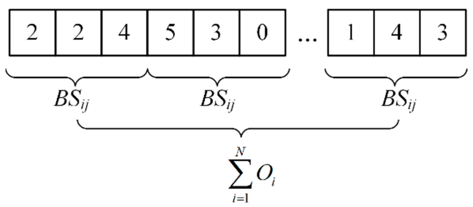
4.2.1. Sublot Splitting Chromosome

The number of sublots, BS_ij, into which each operation is divided, as described in Section 3.3.3, is equal to the sum of the number of machines available for the operation. This is demonstrated by Equation (15).

$$B{S}_{ij}=N{M}_{ij}$$

(15)

In this manner, for the jth process of the job, i, the number of its sublots expressed on the sublot splitting chromosomes is fixed in length. The sublot splitting chromosome are represented in Figure 2.

The sublot splitting chromosomes are initially divided into ${\displaystyle \sum _{i=1}^n{O}_i}$ blocks, arranged in the order of jobs and operations. For instance, the first block represents the sublot scheme for the first operation of job 1, while the second block represents the sublot scheme for the second operation of job 1, and so on. The number of genes in each program block represents the maximum number of sublots that can be divided. Each gene represents the size of a sublot. The second block illustrates this. The gene of the second program block is “5/3/0”, indicating that the second operation of job 1 can be divided into three sublots. Since the third sublot is 0, it is divided into two sublots: the first sublot is 5, and the second sublot is 3.

The main advantage of coding the sublot splitting chromosomes in this way is that it ensures that the length of each individual’s chromosomes remains the same during the iterative process. This consistency facilitates mutation, crossover, and decoding operations, and prevents the generation of illegal solutions.

For simplicity and to ensure the quality of the initial solution, this paper adopts an equal-sized batch splitting scheme to initialize the sublot splitting chromosomes. Each operation’s jobs are divided into sublots of equal size.

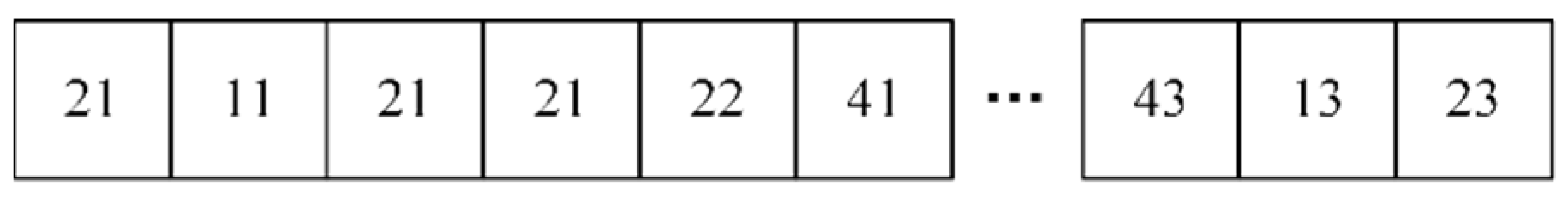
4.2.2. Sublot Sorting Chromosome

The sublot sorting chromosomes list all sublots for each operation of each job. Their function is to sort these sublots, so the lengths of the sublot sorting chromosomes and the sublot sorting chromosomes should be equal. In this paper, a sequential order of appearance is used to encode the sublot splitting chromosomes.

As illustrated in Figure 3, the chromosome is comprised of a total of ${\displaystyle \sum _{i=1}^N{\displaystyle \sum _{j=1}^{O_i}B{S}_{ij}}}$ decimal two-digit numbers. The tens digit of the chromosome indicates the job type to which the current sublots belong. The first digit indicates the number of operations corresponding to the current sublot, and the order of appearance indicates the serial number of the corresponding sublots. For example, the first instance of “21” indicates the first sublot of the first operation of job 2, while the second instance of “21” indicates the second sublot of the first operation of job 2, and so on, until “21” has appeared BS_ij times, indicating that all sublots have been sequenced.

It is crucial to recognize that the number representing the next operation can only appear after the number corresponding to the previous operation of each job has been displayed BS_ij times. As illustrated in Figure 3, “22” only appears after three instances of “21”, and “22” for the subsequent operation cannot appear before any instance of “21”. This is consistent with the constraint in Section 3.3.3, which stipulates that the next operation can only begin once the previous operation of all sublots has been completed.

This two-digit encoding is only suitable for small-scale problems, where both the number of jobs and the number of operations must be less than 10. In contrast, large-scale problems can use four-digit numbers, encoded in the same way. This paper uses two-digit encoding for ease of illustration. Furthermore, the initialization of sublot sorting chromosomes is performed randomly.

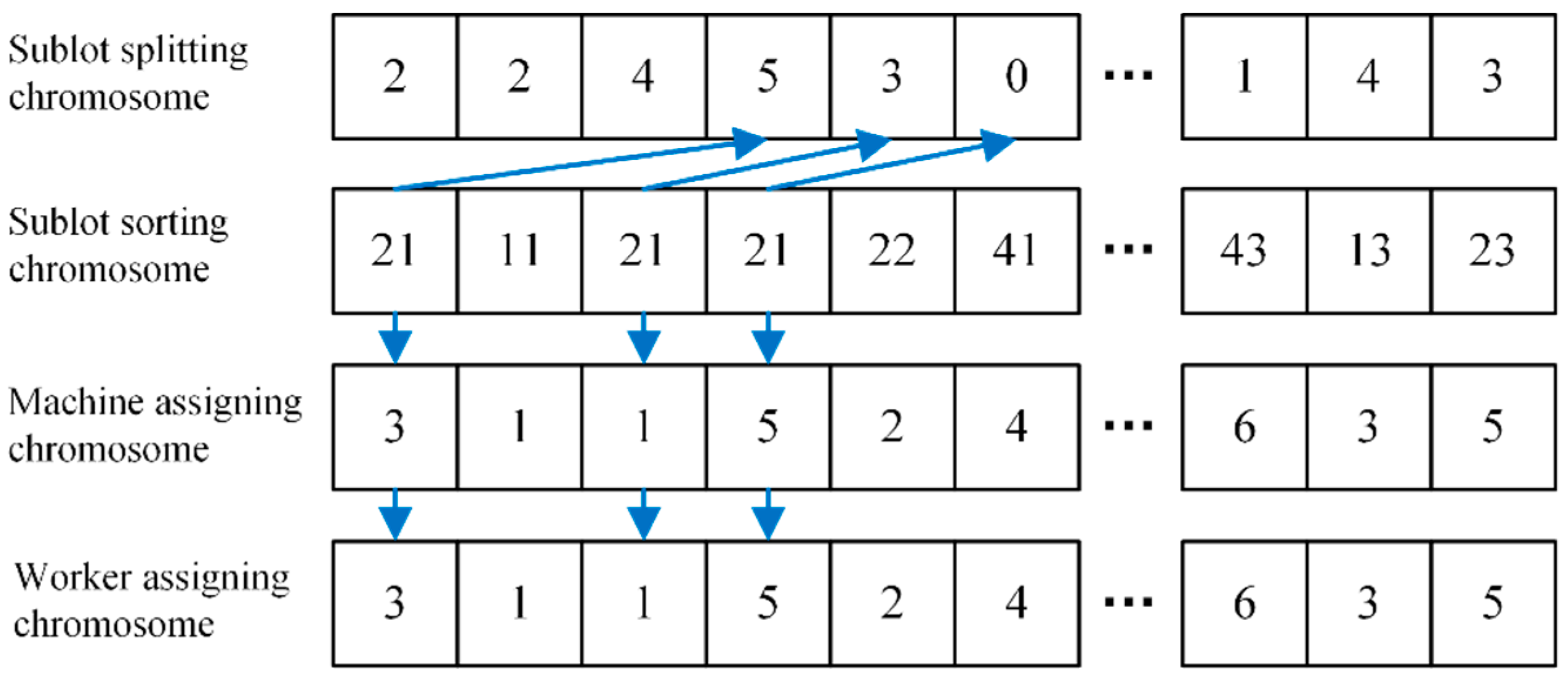
4.2.3. Machine Assigning Chromosomes and Worker Assigning Chromosomes

As shown in Figure 4, machine assigning chromosomes and worker assigning chromosomes are similar in that they are both the same length as sublot sorting chromosomes and sublot splitting chromosomes. Corresponding to the sublot sorting chromosomes, each gene in the machine assigning chromosomes indicates the machine selected for the sublot, and similarly, each gene in the worker assigning chromosomes indicates the worker assigned to the sublot. For example, the first “3” in the machine assigning chromosomes indicates that the sublot selects machine 3 for processing, while the first “1” in the worker assigning chromosomes indicates that the sublot is assigned to worker number 1 for processing. The machine assigning chromosomes and worker assigning chromosomes are initialized in a random manner, taking into account only the processing capacity constraints.

4.2.4. Individual Decoding

An illustration of the decoding process for an individual is shown in Figure 5. During the decoding process, it is necessary to traverse the sublot sorting chromosome. For example, the decoding process for all sublots of the first operation of job 2 is given in the figure. To illustrate, consider the first instance of the digit “21”. The arrows in the figure indicate how “21” corresponds to the sublot splitting chromosome, machine assigning chromosome, and worker assigning chromosome. This digit is represented by the block “5/3/0” in the sublot splitting chromosome. The first instance of “21” in the figure is therefore “5/3/0”. Decoding the machine assigning-chromosomes and worker assigning chromosomes is relatively simple: directly find the corresponding position of the gene, the selected machine is machine 3, and the assigned worker is worker 3.

The processing time of a sublot can be calculated based on the sublot size, the corresponding operation of the job, and the selected machine and worker. The start time of each sublot is determined by the constraints of the end of the current machining time of the machine and worker and the end time of the machining of all sublots from the previous operation. Subsequently, the end processing time of each sublot can be determined. The maximum sublot end processing time represents the primary objective of the research problem, namely the makespan. The processing time of each sublot is aggregated according to the workers, and the maximum processing time of each worker represents the second objective of the research problem, namely the maximum worker working time.

4.3. First-Stage Discrete Multi-Objective Differential Evolution Algorithm

The conventional differential evolutionary algorithm (DEA) typically follows the following standard process:

(1)

A random initial population is generated.

(2)

Mutation of the population.

(3)

Population crossover.

(4)

Processing of boundary conditions and selection of an optimal population.

(5)

Once the predefined termination conditions have been met, the iteration is terminated, and the optimal solution is output.

The mutation and crossover operations typically used in traditional differential evolution algorithms are applied to continuous problems. To effectively address discrete variables and multi-objective optimization challenges, this paper proposes a discrete multi-objective differential evolutionary algorithm. The algorithm considers the characteristics of the discrete problem by appropriately improving the mutation and crossover operations and adopting a Pareto multi-objective optimization strategy to optimize multiple objective functions simultaneously. In this manner, the algorithm can efficiently explore the potential solution space within the discrete search space and identify a set of non-dominated solutions that perform well across multiple objectives.

4.3.1. Adaptive Mutation Operator

The original formula for the adaptive mutation operation in the differential evolutionary algorithm is as follows:

$$V_i^g=X_{r1}^g+F(X_{r2}^g-X_{r3}^g)$$

(16)

where $X_r^g$ denotes the rth individual of the population in generation g, $V_i^g$ denotes the rth individual resulting from the mutation in generation g, and i = 1, 2, 3, …, Np, r1, r2, r3 ∈ [1, Np], r1 ≠ r2 ≠ r3. In the first stage, adaptive mutation evolution operations are required for sublot sorting chromosomes, machine assigning chromosomes, and worker assigning chromosomes. This formula is more effective when dealing with continuous numerical genes, but not for discrete variables. For the discrete problem, we have improved the original variation operator to suit the problem studied in this paper. For the three discrete variables, sublot sorting chromosomes, machine assigning chromosomes, and worker assigning chromosomes, which are involved in the first stage of this paper, the variation of chromosomes has been improved to a kind of variation based on crossover operation. The specific operation steps are as follows:

(1)

The Pareto solution set of the population is calculated, and an individual corresponding to a solution in the solution set of the Pareto front is randomly selected as r1.

(2)

Randomly select two individuals, r2 and r3, from the population that differ from r1, ensuring that r1, r2, r3 ∈ [1, Np], r1 ≠ r2 ≠ r3.

(3)

The precedence operation crossover (POX) is applied to r1 and r2, resulting in the generation of a new individual, rr.

(4)

The desired new mutant individual is obtained by crossing the new individual, rr, with r3 for another POX.

The use of POX crossover is straightforward to implement, and it is effective in preserving the structural characteristics of the paternal chromosomes. Furthermore, this approach ensures the rationality of the offspring chromosomes after crossover to meet the operational constraints.

It is acknowledged that using POX crossover may result in individuals becoming too similar. Therefore, this paper proposes an adaptive POX crossover. During the iteration process, the crossover probability is dynamically adjusted based on the number of evolutionary generations to maintain population diversity and improve search efficiency. Specifically, the initial crossover probability is relatively high, promoting individual diversity. Conversely, the crossover probability gradually decreases with more iterations, thereby retaining the genetic information of good solutions. The specific steps of the improved adaptive POX crossover are as follows:

(1)

The set of jobs is divided into J1 with probability F, while the remainder is J2. The parent chromosomes are designated as p1 and p2, respectively, and the offspring chromosome is designated as cc.

(2)

The operations of jobs in J1 are copied from p1 to cc, with their positions in cc remaining unchanged.

(3)

The operations of jobs in J2 are copied from p2 to cc, with the order in cc remaining unchanged. cc represents the resulting individual after POX crossover.

Figure 6 depicts the adaptive POX crossover plot. Pink and blue represent the genes from the p1 and p2 chromosomes that are selected for crossover and transferred to cc, respectively. The arrows indicate the crossover process. In this crossover, p1 represents the superior parent individual whose genes must be retained. The probability of retaining the p1 gene on the parent chromosome, denoted by F, is given in the following equations:

$$\lambda =e^{1-{\displaystyle \frac{G}{G+1-g}}}$$

(17)

$$F=F_0\times 2^{\lambda }$$

(18)

where F₀ represents the variation operator, G denotes the maximum number of evolutionary generations, and g denotes the current number of evolutionary generations. At the outset of the algorithm, the adaptive mutation operator is set to 2F₀, which is a high value to maintain individual diversity and prevent premature convergence. As the algorithm progresses, the mutation operator is gradually reduced, and the mutation rate approaches F₀ in the later stages to retain beneficial information, prevent the optimal solution from being destroyed, and increase the probability of finding the global optimum.

4.3.2. Adaptive Crossover Operator and Selection Strategy

In addition to mutation, crossover is also a crucial component of differential evolutionary algorithms. The traditional fixed crossover probability may have limitations in addressing different problems. To address this issue, an adaptive stochastic crossover operator is proposed in this paper, as shown in Equation (19).

$$CR=0.5\times [1+rand(0.5,1)]$$

(19)

This approach ensures that the average value of the crossover operator remains at 0.75. The design of the adaptive crossover operator considers maintaining individual diversity throughout the search process and enhancing global search capability. The enhanced adaptive crossover operator also employs the adaptive POX crossover. However, the probability of retaining the p1 gene of the paternal chromosome was changed from F to CR.

The newly obtained chromosomes from the adaptive crossover serve as the basis for the new sublot sorting chromosomes, machine assigning chromosomes, and worker assigning chromosomes. These chromosomes are then recalculated to reflect the values of the two fitness functions corresponding to the new chromosomes. If the new individual dominates the original individual, the three chromosomes of the individual are updated to reflect the new chromosomes. Otherwise, the original chromosomes are retained. This process follows an elitism procedure, ensuring that the best solutions from the current generation are preserved and passed on to the next generation, thus preventing the loss of high-quality solutions and enhancing the overall performance of the algorithm.

4.3.3. Pseudocode of Discrete Multi-Objective Differential Evolution Algorithm

The specific pseudocode of the proposed first-stage discrete multi-objective differential evolution algorithm is shown in Algorithm 1.

Algorithm 1. Procedure of discrete multi-objective differential evolution algorithm

1: For g = 1 to G 2:    For each chromosome_type in sublots_sorting_chromosomes, machines_selecting_chromosomes, workers_assigning_chromosomes 3:     For each individual i in population 4:       Calculate Pareto solution set of the population 5:       Select an individual r1 randomly from Pareto solution set 6:       Select two different individuals r2 and r3 randomly from the population, ensuring r1 ≠ r2 ≠ r3 7:       Perform POX crossover on r1 and r2 to generate a new individual rr 8:       Perform POX crossover on rr and r3 to obtain mutant individual 9:       Perform adaptive POX crossover as follows: 10:         Select jobs into J1 with probability F, remainder into J2 11:         Copy jobs from J1 in p1 to cc, maintaining their positions 12:         Copy jobs from J2 in p2 to cc, maintaining their order 13:       cc = resulting individual after POX crossover 14:       Perform enhanced adaptive crossover operation on mutant individual to generate new chromosomes 15:       Calculate new fitness values for new chromosomes 16:       If new fitness values dominate original fitness values 17:         Update individual chromosomes to new chromosomes 18:       End If 19:     End For 20:   End For 21: End For

4.4. Second-Stage Adaptive Multi-Objective Simulated Annealing Algorithm

In the second stage, iterative optimization is required for the sublot splitting chromosomes to obtain the optimal splitting scheme. In this paper, an adaptive multi-objective simulated annealing algorithm is designed for this subproblem.

4.4.1. Random Disturbance

In the context of simulated annealing iteration, introducing a random perturbation of the chromosome is essential for generating a novel solution. In practical production, machinery processing products often operates on a fixed unit lot, Lp. Consequently, in the design of the perturbation presented in this paper, the unit for perturbation change in sublot splitting chromosomes is also set to Lp. This approach can significantly reduce the search space for sublot splitting chromosomes while simultaneously improving the quality of the solution. The specific method for generating the perturbation is as follows:

(1)

For each operation divided into multiple sublot sets, randomly select two different sublots, s1 and s2.

(2)

If rand (0, 1) > PR and the number of sublots of s1 is greater than or equal to Lp, then the number of sublots of s1 should be decreased by Lp, while the number of sublots of s2 should be increased by Lp. Otherwise, no change should be made.

PR is the probability of generating a disturbance for each operation. The value of Lp is equal to the original lot size of the smallest sublot divided by 100, rounded upward, as illustrated in Equation (20).

$$Lp=⌈{\displaystyle \frac{\underset{i=1}{\overset{N}{\min }}(S_i)}{100}}⌉$$

(20)

This method of generating perturbations not only accelerates the search process by varying the sublot scheme for each operation with a certain probability but also ensures the correctness and reasonableness of the sublot scheme by maintaining a constant sum of sublots for each operation.

4.4.2. Adaptive Acceptance Criterion

The most commonly employed criterion for determining the acceptance or rejection of a novel solution is the Metropolis criterion. If the change in energy (ΔE) is negative, then X′ is accepted as the new current solution X. Otherwise, X′ is accepted as the new current solution X with a probability of exp(−ΔE/T). However, this criterion is only applicable to single-objective optimization problems. For multi-objective problems, some improvement of this acceptance criterion is necessary. The multi-objective Metropolis criterion, as described in this paper, is as follows:

(1)

Calculate the set of Pareto solutions for the mixed population by adding the individuals generated by the random perturbation to the original population.

(2)

Calculate the number of newly generated individuals in the Pareto front solution set as NN and the number of individuals in the Pareto front solution set as FN.

Accept the new solution if NN = FN; otherwise, accept the new solution with a probability of MR.

$$MR=e^{-{\displaystyle \frac{NN-NR}{t}}}$$

(21)

Equation (21) illustrates the value of MR, where the probability of accepting the new solution decreases as the temperature T decreases. The higher the percentage of new individuals in the frontier solution, the higher the probability of accepting the new solution.

4.4.3. Annealing and Termination

In the simulated annealing algorithm, an initial temperature and a termination temperature are set. When the temperature drops below the termination temperature, the simulated annealing algorithm terminates, and no new solutions are searched. In this paper, the following equation is used for the temperature cooling process:

$$T(g+1)=K\times T\left(g\right)$$

(22)

where 0 < K < 1. This cooling process occurs in the iterative loop of the differential evolution algorithm, meaning that the temperature of the simulated annealing algorithm decreases with each iteration of the differential evolution algorithm. When the temperature is less than the termination temperature, it indicates that the optimal batch scheme has been found. From then on, the batch scheme remains unchanged while only iterations of the differential evolution algorithm continue. Usually, to ensure a thorough search, the initial temperature T is set higher. To improve search efficiency and reduce solution space complexity, this paper also introduces a new termination strategy. The termination strategy is as follows:

(1)

Two consecutive temperature drops are performed, each with a number of iterations equal to the Markov chain length L.

(2)

The simulated annealing algorithm terminates if the number of newly generated individuals, NN, in the Pareto front solution set is zero for each iteration.

The newly implemented termination strategy ensures that the search for a superior batch program is concluded in a timely manner. This not only guarantees the retention of the superior batch program but also reduces unnecessary expenditure of search resources.

4.4.4. Pseudocode of Adaptive Simulated Annealing Algorithm

The specific pseudocode of the proposed second-stage adaptive multi-objective simulated annealing algorithm is shown in Algorithm 2.

Algorithm 2. Procedure of adaptive simulated annealing algorithm

1: WHILE T > T_term AND N_iterations < max_iterations AND NOT EarlyTermination DO 2:   NN_previous = 0 3:   FOR each solution X in population P DO 4:     FOR i = 1 TO L DO 5:       Generate a random perturbation for X: 6:         For each operation divided into multiple sublot sets: 7:           Randomly select two different sublots s1, s2. 8:           IF rand(0, 1) > PR AND number of sublots of s1 ≥ Lp THEN 9:             Decrease the number of sublots of s1 by Lp. 10:             Increase the number of sublots of s2 by Lp. 11:       Calculate the energy difference ΔE between X and X’ (perturbed solution). 12:       IF ΔE < 0 OR (NN = FN) OR (rand(0, 1) < exp(-ΔE/T)) THEN 13:         Accept X’ as the new current solution X. 14:         Update population P with X’. 15:         Update Pareto front solutions. 16:         Update NN and FN based on the new solutions in the Pareto front. 17:       END IF 18:     END FOR 19:   END FOR 20:   Update temperature T using cooling schedule T = T × K. 21:   IF NN > 0 THEN 22:     N_iterations = 0 23:   ELSE 24:     N_iterations = N_iterations + 1 25:   END IF 26:   IF NN_previous == 0 AND NN == 0 THEN 27:     N_consecutive = N_consecutive + 1 28:     IF N_consecutive >= 2 THEN 29:       EarlyTermination = true 30:     END IF 31:   ELSE 32:     N_consecutive = 0 33:   END IF 34:   NN_previous = NN 35: END WHILE

5. Experiments and Analysis

In this paper, we have designed several sets of experiments for the mixed-integer linear programming model and the TSMOEA algorithm proposed for the DRCFJSP-VS problem to verify the reliability of the model and the stability and efficiency of the algorithm, and the designed experiments are all programmed in Python 3.7 and run on a computer with 8 G of RAM and a 2.3 Ghz CPU.

5.1. Validation of the Proposed MILP Model

In order to verify the validity of the proposed mixed-integer linear programming (MILP) model, this paper employs IBM’s CPLEX optimization solver to solve the model. CPLEX, as an industry-leading commercial optimization software, is capable of efficiently dealing with all kinds of linear and integer programming problems due to its excellent performance. The CPLEX solver was employed to obtain optimal or near-optimal solutions to the MILP model, which will serve as important benchmarks for subsequent comparative analyses.

Given the potential difficulties CPLEX may encounter when addressing large-scale problems, a small-scale arithmetic instance drawn from real-world production has been selected for comparative analysis in this paper. The specific data for the arithmetic case are presented in

Table 2. Unit processing time for operations on alternative machines and original sublot size of the jobs.

Job	Operation	Machine			Original Sublot Size
		M1	M2	M3
J1	1	2	3	4	5
	2	-	3	4
	3	1	4	5
J2	1	3	-	5	5
	2	4	3	-
	3	5	-	4
J3	1	5	6	-	5
	2	-	4	1
	3	2	-	13

and

Table 3. Efficiency of workers operating machines.

Worker	Machine
	M1	M2	M3
W1	6	-	-
W2	1	2	1

. Table 2 lists the time required for the jobs to be processed by the selected machine under different operations, as well as the original sublot size of the jobs. Table 3 reflects the coefficients of the workers’ ability to operate the different machines, with larger coefficients indicating that the worker is less proficient in operating the machine. In the table, “-” indicates that the machine is not able to process the operation or the worker is not able to operate the machine.

The two-stage multi-objective evolutionary algorithm (TSMOEA) proposed in this paper is then applied to the algorithmic example and compared with the solution results from CPLEX. The Pareto front solutions for both are computed and plotted as line graphs for visualization (as shown in Figure 7). The blue points in the figure represent the Pareto frontier solutions solved by CPLEX, while the orange points represent the frontier solutions solved by TSMOEA. Although the solutions produced by CPLEX exhibit slightly superior performance, the discrepancy between the two is not substantial. This substantiates the MILP model developed in this paper and demonstrates that TSMOEA is comparable to CPLEX in terms of performance on small-scale problems, thereby corroborating its excellent efficacy.

In the context of small-scale problems, CPLEX is unquestionably effective. However, when confronted with large-scale problems, the solution time of CPLEX tends to increase significantly, making it challenging to guarantee the attainment of a global optimal solution. In contrast, the TSMOEA algorithm proposed in this paper is well-suited to address this challenge and offers an efficacious solution for the resolution of large-scale problems.

5.2. Experimental Test Instances

This paper explores the dual-resource constrained flexible job shop scheduling problem with variable sublots (DRCFJSP-VS), an area that remains underexplored. As a result, comprehensive and standardized test instances for direct reference are scarce. To thoroughly evaluate the effectiveness and performance of the proposed algorithm, we have meticulously enhanced and expanded the standardized test instances originally designed by Brandimarte [31] and Dauzere-Peres et al. [32]. Specifically, we have constructed 28 new test instances by introducing key parameters such as the original batch size of the job (S_job), the number of workers (N_worker), and the efficiency of workers operating machines (E_worker). These parameters were varied randomly to create a diverse set of scenarios. The details of these arithmetic instances are presented in

Table 4. Parameters of the instances.

Instance	N_job	N_mac	N_op	T_proc	S_job	N_worker	E_worker
Mk01	10	6	5–7	1–7	20–30	3	1–5
Mk02	10	6	5–7	1–7	20–30	3	1–5
Mk03	15	8	10–10	1–20	20–50	4	1–5
Mk04	15	8	3–10	1–10	20–50	4	1–5
Mk05	15	4	5–10	5–10	20–50	2	1–5
Mk06	10	15	15–15	1–10	30–60	9	1–5
Mk07	20	5	5–5	1–20	10–30	3	1–5
Mk08	20	10	10–15	5–20	20–50	6	1–5
Mk09	20	10	10–15	5–20	20–50	6	1–5
Mk10	20	15	10–15	5–20	30–60	9	1–5
01a	10	5	15–25	10–100	10–30	3	1–5
02a	10	5	15–25	10–100	10–30	3	1–5
03a	10	5	15–25	10–100	10–30	3	1–5
04a	10	5	15–25	10–100	10–30	3	1–5
05a	10	5	15–25	10–100	10–30	3	1–5
06a	10	5	15–25	10–100	10–30	3	1–5
07a	15	8	15–25	10–100	20–50	4	1–5
08a	15	8	15–25	10–100	20–50	4	1–5
09a	15	8	15–25	10–100	20–50	4	1–5
10a	15	8	15–25	10–100	20–50	4	1–5
11a	15	8	15–25	10–100	20–50	4	1–5
12a	15	8	15–25	10–100	20–50	4	1–5
13a	20	10	20–25	10–100	20–50	6	1–5
14a	20	10	20–25	10–100	20–50	6	1–5
15a	20	10	20–25	10–100	20–50	6	1–5
16a	20	10	20–25	10–100	20–50	6	1–5
17a	20	10	20–25	10–100	20–50	6	1–5
18a	20	10	20–25	10–100	20–50	6	1–5

. This curated set of instances provides a robust foundation for our investigation and enables a precise assessment and improvement of the proposed scheduling algorithm.

5.3. Parameter Settings and Design of Experiment

In order to ensure the diversity of the population and adequate search of the algorithm, this paper empirically sets the size of the population, Np, to 100, the number of iterations, G, of the differential evolutionary algorithm to 100, the decay parameter, K, of the temperature to 0.99, and the termination temperature to T₀ = 0.001.

In addition, three key parameters must be determined: the variation operator F₀ underlying the differential evolution algorithm, the initial temperature T for simulated annealing, and the length L of the Markov chain to be searched for each temperature. The probability of retaining the optimal parent genes is determined by F₀, the probability of the algorithm accepting an inferior solution is determined by T, and L ensures that each temperature is adequately searched. Failure to adequately search for the optimal solution will cause the simulated annealing to terminate prematurely, thus missing the optimal solution. In this paper, this is determined using the design of experiment (DOE) method using instance mk02 in 5.2. For each of the three parameters, four parameter levels were selected, as shown in

Table 5. Values for each parameter level.

Parameter	Level
	1	2	3	4
F0	0.2	0.3	0.4	0.5
T	50	100	150	200
L	10	50	100	150

.

Based on the number of parameters and the number of levels, an orthogonal test of size L₁₆(4³) is selected, as shown in

Table 6. Orthogonal table with response values (RV).

Combination	Level			RV
	F0	T	L
1	1	1	1	0.047921
2	1	2	2	0.004999
3	1	3	3	0.047157
4	1	4	4	0.133573
5	2	1	2	0.114737
6	2	2	1	0.083984
7	2	3	4	0.136632
8	2	4	3	0.086523
9	3	1	3	0.126906
10	3	2	4	0.150938
11	3	3	1	0.111776
12	3	4	2	0.188978
13	4	1	4	0.248811
14	4	2	3	0.222186
15	4	3	2	0.241105
16	4	4	1	0.358258

. The TSMOEA is run 20 times for each combination of parameter levels, and the average of the IGDs obtained from these 20 runs is taken as the response value (RV) for the current combination.

As illustrated in

Table 7. Mean response values, range, and significance of each parameter.

Level	F0	T	L
1	0.058413	0.134619	0.150485
2	0.108219	0.115527	0.137455
3	0.144650	0.134168	0.120693
4	0.267590	0.191833	0.167489
Range	0.209177	0.076306	0.046796
Significance	1	2	3

of the results of orthogonal experiments, the response values of the four tests corresponding to each level of each parameter are averaged (with six decimals retained) and recorded as the average response value for each parameter. The difference between the maximum and minimum values of the average response values for each parameter was calculated as the range, and the ranges were ranked in descending order to indicate the significance of each parameter.

The parameter F₀ has the greatest range, thus exerting the most significant influence on the performance of the algorithm. If F₀ assumes an excessively large value, it will prompt the algorithm to converge prematurely and settle into a local optimum solution. To facilitate analysis, the average response values presented in Table 7 are plotted as a line graph, as illustrated in Figure 8.

As illustrated in Figure 8, the smaller the average response value of each parameter, the more effective the algorithm. Therefore, each parameter of the TSMOEA algorithm proposed in this paper is selected as follows: the base variance factor F₀ = 0.2 for the differential evolution algorithm, the starting temperature T = 100 for the simulated annealing algorithm, and the length of the Markov chain for each temperature search, L = 100.

5.4. Comparative Analysis of TSMOEA Variants and Other Algorithms

In order to verify the effectiveness of the improved mutation operator, improved crossover operator, and improved simulated annealing algorithm, this paper introduces additional experiments involving the two-stage multi-objective evolutionary algorithm (TSMOEA) with traditional mutation, TSMOEA with traditional crossover, and TSMOEA with traditional simulated annealing. These experiments aim to evaluate the performance of the proposed improvements. For the traditional mutation operator (TSMOEA-TM), the parameters are set according to common values used in differential evolution: mutation factor (F) = 0.5. For the traditional crossover operator (TSMOEA-TC), the crossover probability (CR) is set to 0.9, which is the probability with which the crossover operation is applied to the individuals. For the traditional simulated annealing (TSMOEA-TSA), the initial temperature (T₀) is set to 1000, the cooling rate (K) is set to 0.99, with a maximum of 500 iterations per temperature level, and the stopping criterion is when the temperature drops below a threshold (typically 0.001) or after a fixed number of iterations.

In addition, the TSMOEA proposed in this paper is compared with several widely used algorithms for solving the job shop scheduling problem, including the non-dominated sorting genetic algorithm II (NSGA-II, Fan et al. [33]), particle swarm optimization (PSO, Zhou et al. [34]) algorithm, the grey wolf optimizer (GWO, Arani et al. [35]) algorithm, and the whale optimization algorithm (WOA, Li et al. [36]). These algorithms are applied to the test instances introduced in Section 5.2 for comparison. Since none of these algorithms directly address the dual-resource constraints with variable-sized batch splitting and worker capacity, necessary modifications are made by introducing sublot splitting chromosomes and worker assigning chromosomes to adapt these algorithms to the problem at hand. The original parameter settings for each algorithm are adopted as recommended in their respective reference papers.

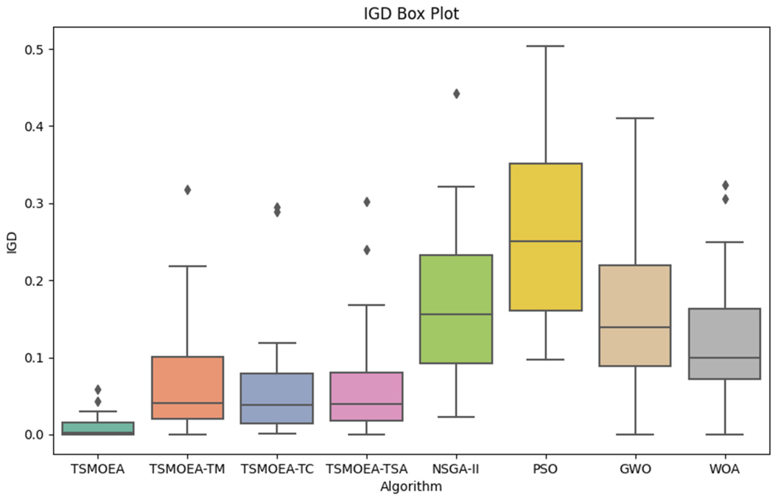
In order to evaluate the comprehensive performance of the algorithms, two commonly used metrics in multi-objective optimization, Inverted Generational Distance (IGD) and Hypervolume (HV), are selected. The IGD metric measures the minimum Euclidean distance from the true Pareto front to the solution set, focusing on both convergence and distribution, with a smaller IGD value indicating better algorithm performance. The HV metric measures the volume of the region in the objective space enclosed by the set of non-dominated solutions obtained by the algorithm and a reference point. The larger the HV value, the better the comprehensive performance of the algorithm.

TSMOEA and its variants (TSMOEA-TM, TSMOEA-TC, and TSMOEA-TSA), along with the other four comparison algorithms (NSGA-II, PSO, GWO, and WOA), were each run 20 times on each dataset. The average IGD and HV values obtained from these experiments are recorded in

Table 8. Comparison of IGD and HV across TSMOEA variants and other algorithms.

Instance	TSMOEA		TSMOEA-TM		TSMOEA-TC		TSMOEA-TSA		NSGA-II		GWO		PSO		WOA
	IGD	HV	IGD	HV	IGD	HV	IGD	HV	IGD	HV	IGD	HV	IGD	HV	IGD	HV
Mk01	0.015066	0.901238	0.005264	0.929371	0.088924	0.868614	0.030977	0.874758	0.157889	0.499998	0.257746	0.304812	0.249907	0.282069	0.161001	0.424636
Mk02	0	0.898609	0.063294	0.516263	0.067182	0.563932	0.075260	0.563422	0.022857	0.827716	0.136181	0.379389	0.256468	0.036389	0.041803	0.501576
Mk03	0.024009	0.955967	0.006734	0.792046	0.004555	0.789535	0.008183	0.846337	0.320904	0.221273	0.217068	0.419822	0.458481	0.131240	0.117209	0.550889
Mk04	0	0.978422	0.061947	0.707902	0.036589	0.751395	0.128002	0.752443	0.267060	0.268680	0.225354	0.238020	0.382314	0.085622	0.306092	0.208340
Mk05	0	0.960568	0.134009	0.910040	0.018584	0.898735	0	0.948990	0.093426	0.196296	0.104116	0.168937	0.180222	0.004711	0.079922	0.324009
Mk06	0.002473	0.942706	0.020196	0.729928	0.100283	0.570502	0.037906	0.766022	0.172698	0.511948	0.140882	0.538556	0.340248	0.322551	0.132881	0.592714
Mk07	0.008107	0.917699	0.137768	0.601032	0.048687	0.749773	0	0.909791	0.265246	0.333503	0.273439	0.340008	0.393497	0.176583	0.179112	0.454903
Mk08	0	0.988698	0.161522	0.744931	0.113398	0.748055	0.148291	0.730732	0.288912	0.312879	0.257904	0.400792	0.388265	0.162595	0.249664	0.417065
Mk09	0	0.959038	0.019677	0.568461	0.004983	0.592744	0.030597	0.543730	0.169992	0.281720	0.182036	0.324446	0.324210	0.127330	0.154494	0.395494
Mk10	0	0.987510	0.317261	0.306186	0.294743	0.341758	0.239353	0.385769	0.442485	0.158389	0.410572	0.185924	0.503626	0.052878	0.324032	0.299324
01a	0.015979	0.959067	0.036824	0.774419	0.028077	0.741108	0.133518	0.801326	0.083416	0.705053	0.081190	0.598625	0.132939	0.480743	0.076356	0.673370
02a	0	0.943738	0.044938	0.475269	0.027513	0.463813	0.069022	0.510930	0.065438	0.411830	0.093167	0.309652	0.156466	0.275872	0.090980	0.393970
03a	0	0.997825	0.218127	0.546604	0.288422	0.558600	0.301772	0.698345	0.226792	0.419937	0.141530	0.512333	0.218355	0.335066	0.104081	0.555636
04a	0.022111	0.896059	0.060053	0.567899	0.008346	0.572826	0.021644	0.740943	0.049269	0.486362	0.073255	0.375235	0.162565	0.108880	0.063402	0.427093
05a	0.058620	0.905026	0.117796	0.666015	0.095299	0.704073	0	0.973926	0.171846	0.522071	0.178185	0.375816	0.314826	0.084347	0.150632	0.304580
06a	0.030143	0.900466	0.020424	0.640322	0.022252	0.658351	0.031262	0.771135	0.075989	0.517259	0.056867	0.538818	0.156931	0.241806	0.057694	0.614797
07a	0.020036	0.915209	0.032785	0.595651	0.001114	0.661170	0.075059	0.640763	0.129467	0.495024	0.104347	0.484245	0.304540	0.285816	0.073777	0.508035
08a	0.008294	0.904114	0.053675	0.485651	0.050705	0.500444	0.006014	0.655691	0.095891	0.471067	0.151432	0.442195	0.251452	0.247954	0.123179	0.450686
09a	0	0.989312	0.094522	0.560766	0.075478	0.612311	0.095257	0.646765	0.159676	0.415084	0.197368	0.498240	0.316631	0.254899	0.193876	0.479954
10a	0.006597	0.940452	0.008109	0.389829	0.009592	0.368546	0.019218	0.489516	0.085469	0.255734	0.076441	0.335403	0.111924	0.191725	0.068242	0.288458
11a	0.042719	0.891205	0	0.463601	0.007173	0.463898	0.050068	0.426795	0.113124	0.223620	0.098648	0.339055	0.181063	0.206320	0.093776	0.356218
12a	0.002802	0.967414	0.013750	0.539287	0.011124	0.634204	0.023793	0.485405	0.088668	0.419489	0.091215	0.648001	0.233756	0.200376	0.083971	0.603974
13a	0	0.961253	0.043377	0.647279	0.014816	0.618142	0.010572	0.664390	0.248331	0.311602	0.252293	0.374776	0.392387	0.224023	0.182612	0.510404
14a	0.002487	0.975126	0.030483	0.540317	0.041119	0.564813	0.044723	0.525114	0.263899	0.373520	0.231790	0.506012	0.457908	0.270219	0.169682	0.569691
15a	0	0.846662	0.027463	0.643382	0.021769	0.656982	0.067131	0.512713	0.125400	0.357296	0.011246	0.562340	0.103115	0.228103	0	0.656050
16a	0.007462	0.901413	0.028110	0.542673	0.046558	0.465484	0.015143	0.570446	0.154792	0.235664	0.095483	0.369421	0.164459	0.165268	0.094870	0.371135
17a	0	0.895438	0.038635	0.669914	0.039588	0.631141	0.040372	0.619718	0.133174	0.330667	0	0.594621	0.147308	0.231925	0.065447	0.585093
18a	0	0.850859	0.184219	0.381847	0.119059	0.533549	0.167453	0.573527	0.194483	0.277285	0	0.675865	0.096987	0.203051	0.017015	0.591780

.

In order to facilitate the analysis of the stability and efficiency of each algorithm, the data in Table 8 are plotted as a box plot, as shown in Figure 9 and Figure 10.

It can be seen that TSMOEA has the smallest median average IGD value and the smallest lower and upper edges of the box plots, while the median average HV is the largest, and the lower and upper edges of the box plots are the widest. This indicates that TSMOEA outperforms other algorithms in terms of optimality-seeking ability. Notably, the improvements made to the mutation operator, crossover operator, and simulated annealing algorithm contribute significantly to this performance. The adaptive mutation operator helps the algorithm explore a broader search space, while the adaptive crossover operator facilitates better solution combinations. Furthermore, the improved simulated annealing algorithm enhances the algorithm’s ability to escape local optima and reach more optimal solutions. In addition, the IGD and HV box plots of TSMOEA are the shortest, indicating that its solutions are more centralized and that its stability is better than that of other algorithms.

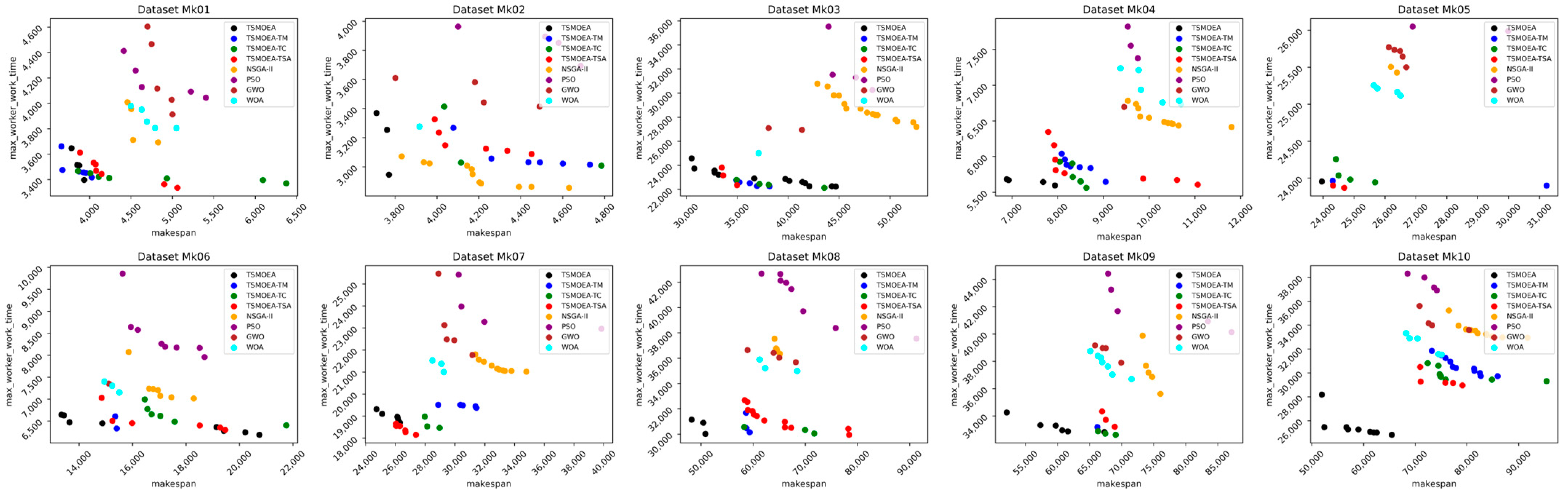
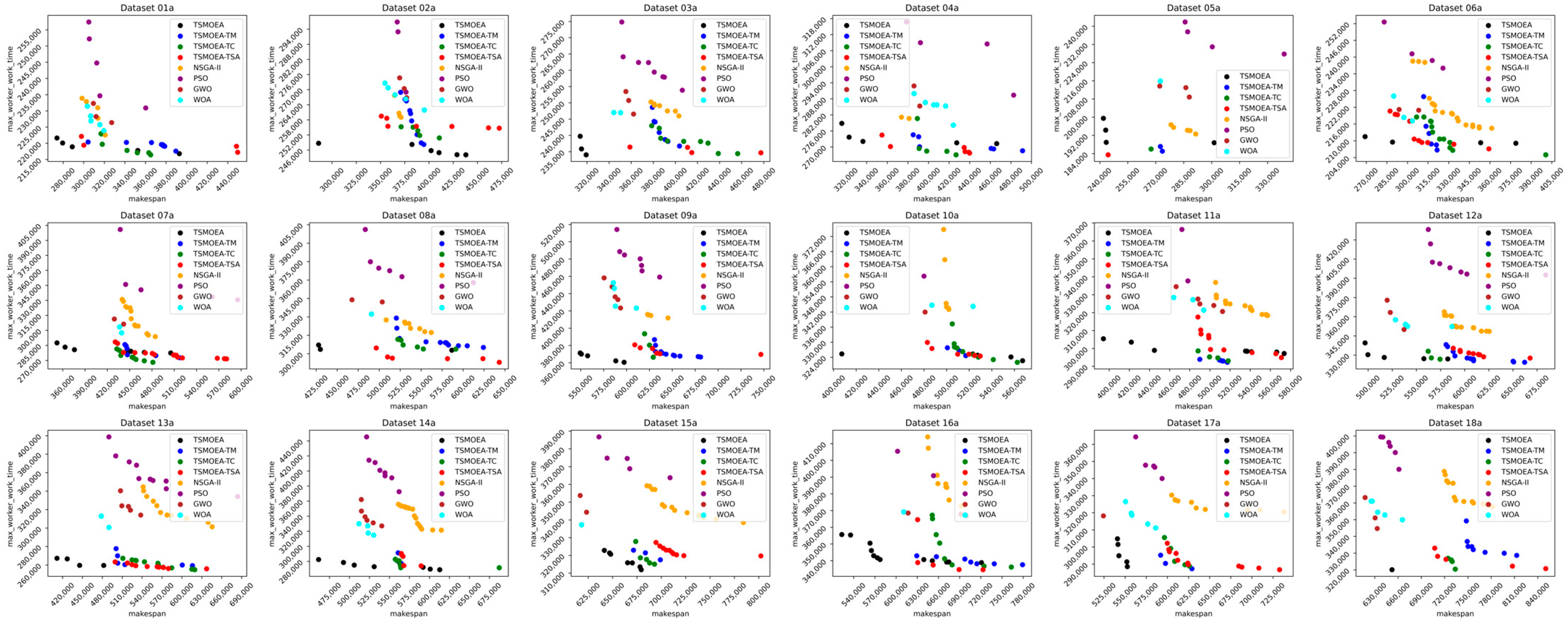
To more clearly compare the effects of the five algorithms on different datasets, scatter plots of the Pareto front solutions obtained by each algorithm are shown in Figure 11 and Figure 12.

Overall, the TSMOEA algorithm proposed in this paper exhibited better optimization ability and algorithmic stability in solving the DRCFJSP-VS, effectively solving this problem.

6. Conclusions

In conclusion, this study has made significant progress in addressing the dual-resource constrained flexible job shop scheduling problem with variable sublots (DRCFJSP-VS) by integrating variable sub-batching alongside dual constraints on human and machine resources. The proposed MILP model and two-stage multi-objective evolutionary algorithm (TSMOEA) effectively optimize scheduling under these complex conditions. The TSMOEA incorporates an adaptive mutation operator and adaptive crossover, and it handles dual-resource constraints, which significantly enhance the solution quality for real-world scheduling problems.

However, this study has limitations. It did not consider buffer management between machines, which could lead to blockages. Given that buffer capacity can greatly influence sublot splitting, its inclusion could further improve the robustness of the model. Additionally, unforeseen events, such as worker illness or fatigue, were not incorporated, potentially impacting processing efficiency.

Future research should consider integrating buffer constraints and dynamically adjusting sublot splitting strategies according to buffer capacity. Furthermore, incorporating workers’ adaptability to unforeseen circumstances is essential for improving the practical applicability and flexibility of scheduling solutions, particularly in dynamic environments.