Data-Driven Soft Sensor Model Based on Multi-Timescale Feature Fusion for Crystal Quality Prediction in Czochralski Process

Abstract

The accurate real-time prediction of the crystal quality index v/G is an important reference for the real-time monitoring of the growth quality status and the process optimization adjustment of semiconductor silicon single crystals. This paper proposes a data-driven crystal quality indicator v/G soft sensor prediction model based on multi-timescale feature fusion to achieve the effective prediction of the crystal quality indicator v/G. Firstly, the characteristics of the crystal quality index v/G in the growth process of Czochralski silicon single crystal are analyzed. Secondly, the crystal quality index v/G is broken down into several natural components using something called complete ensemble empirical mode decomposition with adaptive noise (CEEMDAD), which provides more stable data. On this basis, each intrinsic mode component is reconstructed according to the sample entropy. Then, the maximum mutual information coefficient (MIC) method is applied to identify the characteristic variables most closely associated with each reconstructed component of the crystal quality index v/G from the process-influencing factors. Then, a long short-term memory network with a self-attention mechanism is used to establish a prediction model of the reconstructed components to extract the multi-timescale feature information from the different components of the crystal quality index v/G. Finally, the prediction results of the crystal quality index v/G are obtained by fusing each subsequent prediction model. According to the actual field data, the comprehensive experimental results validate the efficacy of the proposed soft sensor modeling method for the crystal quality index v/G. Compared with the single model, the proposed prediction model has a smaller MAE, RMSE, and prediction performance index and a higher HR prediction hit rate.

1. Introduction

Semiconductor silicon single crystal (SSC) is the key material for the fabrication of integrated circuit chips [1]. At present, the Czochralski (Cz) method is the main technology for preparing high-quality semiconductor SSC. However, the advancements in chip performance introduce more stringent demands regarding the quality of semiconductor SSC [2,3]. Therefore, understanding how to detect or predict the crystal’s quality in real time during the preparation of Cz-SSC can not only help the industrial site to evaluate the current growth state of SSC to optimize the crystal growth process but also affect the smooth operation of the SSC growth control system. This is of great significance for improving the production yield of semiconductor SSC manufacturing enterprises.

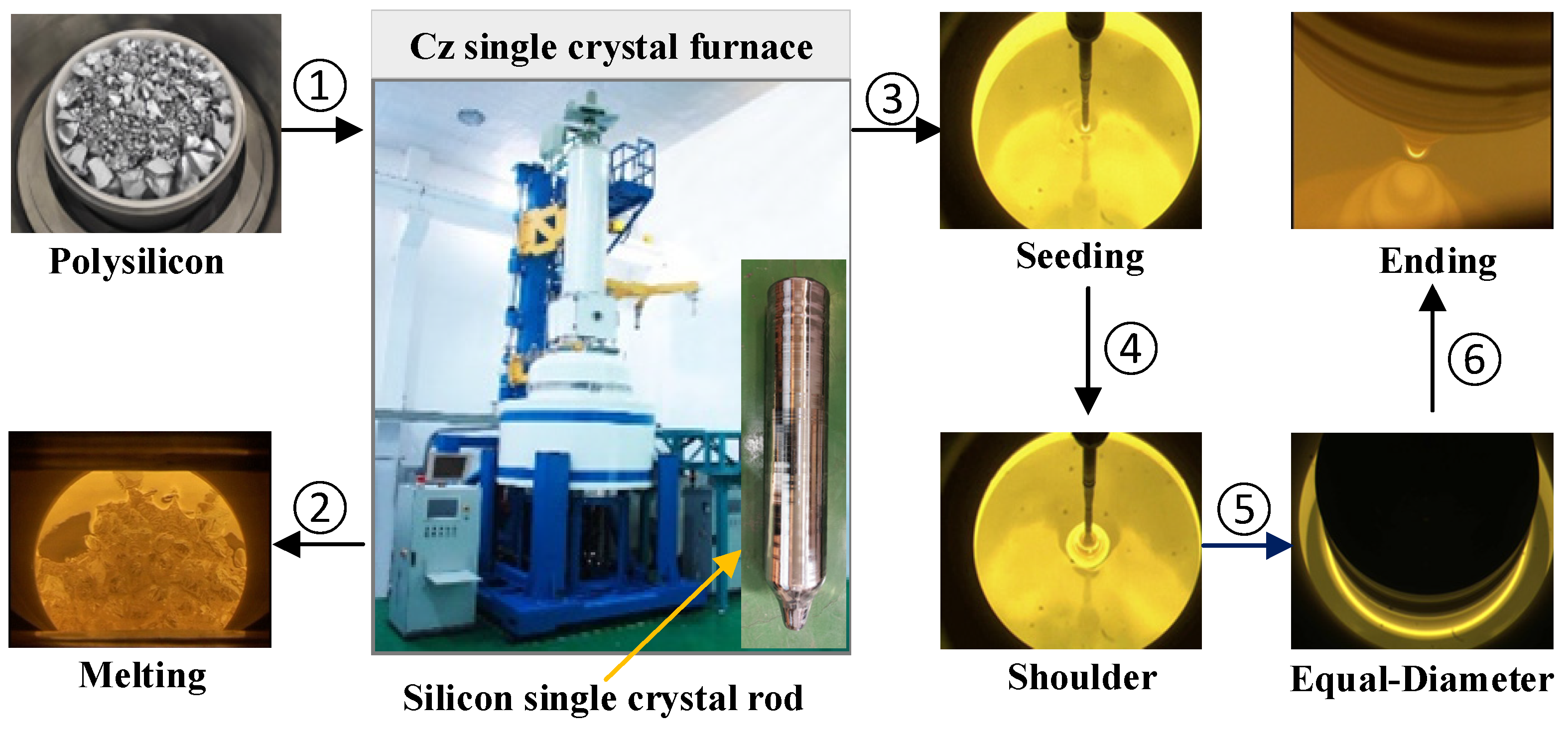
The essence of Cz-SSC growth is a complex physical change process of continuous solid–liquid phase transition. The whole growth process of SSC is completed in a single crystal furnace with a high temperature, vacuum, and magnetic field environment. Figure 1 shows the growth process of Cz-SSC. Firstly, a quartz crucible should be used to contain the high-purity polysilicon, which is subsequently heated and melted with the aid of a graphite heater in a controlled argon atmosphere. When the temperature of the melt tends to be stable (the melting point is about 1412 °C), the rotating seed rod can be inserted into the silicon melt. The melt will crystallize on the seed crystal during a slight temperature drop. By slowly pulling up the seed crystal, the SSC rod hanging on the seed crystal will begin to form. Finally, by adjusting the temperature, the SSC can be grown with a constant diameter size [4]. The whole growth process of the Cz-SSC includes four main stages: seeding, shouldering, equal-diameter, and ending. Among them, the equal-diameter growth phase is central to the entire SSC development process, as it influences both the quality of the final SSC product and the efficiency of the subsequent processing stages [5]. It can be seen that in the growth process of Cz-SSC, ensuring that the quality index of the grown SSC meets the industry requirements from the beginning to the end will be a challenging task for enterprise production.

In the growth process of Cz-SSC, the crystal quality index is mainly reflected in two aspects: shape size and crystal defect. Among them, the shape size mainly refers to the crystal diameter. The crystal defect index mainly refers to the primary point defects inside the crystal, including vacancy enrichment and the self-interstitial, which are formed during the crystallization of SSC. The prediction of the crystal diameter mainly includes the prediction modeling method, based on the first principle [6], and the data-driven prediction modeling method [7]. Among them, the first-principle-based crystal diameter model is constructed based on the principles of physics and heat transfer, which gives the first-principle model a strong theoretical foundation and enables it to accurately describe the inter-relationships between physical variables. However, since the Cz process is an extremely complex physical and chemical reaction process involving gas, liquid, and solid phases and their coupling, it is difficult to quickly establish these models for estimating or predicting the crystal diameter. Thanks to the effective use of distributed control systems and the industrial internet, the Cz-SSC growth system has gathered a significant amount of experimental data that illustrate the conditions of the crystal growth process. In this case, the data-driven modeling method is becoming a powerful candidate for characterizing the state of the complex Cz-SSC growth process [8]. At present, there have been many studies on the prediction modeling of crystal diameter index, but there are few reports on the study of crystal defects. For crystal defects, it is usually desirable to grow SSC native point defects in a reasonable range, ensuring that the crystal has the least “crystal originated particles” and dislocation clusters. Unfortunately, there is currently no effective technical means to directly detect the native point defects of SSC during the growth of Cz-SSC. Consequently, the v/G criterion theory introduced by Voronkov in 1982 was employed to determine whether the main point defects of the SSC extracted from the melt are characterized by an abundance of vacancies or self-interstitials [9,10]. Here, v is the pulling rate of the crystal, and G is the temperature gradient of the crystal growth interface. Since the mid-1990s, the theory of the v/G criterion has served as the foundation for creating silicon crystals and wafers that are free from intrinsic point defect clusters, commonly referred to as “perfect silicon” [11]. Therefore, the v/G value can be utilized as the primary index to evaluate the quality of SSC, and its real-time prediction is pivotal to ensure the sustained growth of high-quality SSC. More importantly, understanding how to realize the accurate prediction of the v/G value in the whole growth process of Cz-SSC is very important to guide the field engineers to adjust the crystal growth process parameters correctly.

Although the v/G value index can evaluate the quality of SSC well [12,13], it cannot be directly measured by hard sensors. Therefore, data-driven soft sensor modeling technology has become an effective means. Compared with traditional hard sensors, soft sensors use advanced modeling techniques to estimate or predict target variables by modeling existing industrial process data [14]. The soft sensor modeling approach, which is based on data, does not necessitate the precise and detailed prior knowledge of crystal growth. Instead, it can anticipate crystal quality parameters solely by utilizing historical data from the operational process. To this end, Wan et al. [15] used the deep learning stacked autoencoder to realize the online prediction task for v/G value variables of difficult crystal qualities according to the easy-to-measure process variables, which showed more accurate prediction results than the shallow network. Currently, the deep learning method has just started being utilized in the modeling research of the Cz-SSC growth process, especially in the prediction of the v/G value index. The existing v/G value index prediction modeling method, based on deep learning, belongs to a single model and may learn features that are independent of specific key variables during model training. It is worth noting that in the Cz process, the sampling frequency and action time of different process variables are different, resulting in multiple timescale data comprehensively affecting the v/G value change process. Therefore, the comprehensive effect of multi-timescale data in the growth process of Cz-SSC must be considered to improve the accuracy of the existing v/G value prediction model. In addition, a data-driven soft sensor modeling method must be developed for the v/G value in the growth process of Cz-SSC, which can realize the real-time online prediction of the change in the crystal quality index v/G and overcome the limitation of the original point defect of SSC not being directly detected by physical sensors.

Inspired by data-driven soft sensor modeling, to solve the above issues, this paper proposes a data-driven soft sensor model based on multi-timescale feature fusion for the prediction of the v/G value. The proposed soft sensor modeling method aims to address the limitations of the traditional model, namely the single prediction result and the absence of time-related feature extraction, with the objective of enhancing the processing of nonlinear and multi-timescale data. The simulation data in this paper are derived from actual semiconductor SSC growth experimental data. The data-driven soft sensor model is focused on the crystal quality index v/G in the equal-diameter growth stage of the Cz process, and the simulation results confirm that the extracted multi-timescale data features can improve the accuracy of the v/G soft sensor model. The main contributions of this study are summarized as follows:

(1)

The v/G data components with different frequencies are obtained by the CEEMDAD decomposition method. Then, different frequency components are reconstructed based on sample entropy, and v/G data sub-sequences with different timescale features are obtained. Finally, based on the MIC method, the characteristic variables with strong correlations with v/G component sequences at different timescales are obtained.

(2)

By adding a self-attention mechanism to the LSTM network, the time–dependence relationships between the v/G data sub-sequences of different timescale features can be effectively captured. The model (referred to as LSTM-SA) has been demonstrated to fully extract the inherent nonlinear and temporal features present in v/G data, thereby achieving enhanced prediction accuracy.

(3)

The LSTM-SA prediction sub-models corresponding to different timescale features are fused to reduce the variance of a single model, enhance the generalization ability, make it more reliable, and further improve the overall prediction performance of the crystal quality index v/G prediction model.

This paper is structured as follows: Section 2 presents a description of the v/G criterion along with the design of the prediction strategy in the Cz process. The procedure for implementing the data-driven soft sensor model that utilizes multi-timescale feature fusion is detailed in Section 3. The results from the experiments and their analyses can be found in Section 4. Lastly, Section 5 presents the conclusions of the research.

2. v/G Criterion Description and Prediction Strategy of Cz Process

2.1. The v/G Criterion Description of Cz Processes

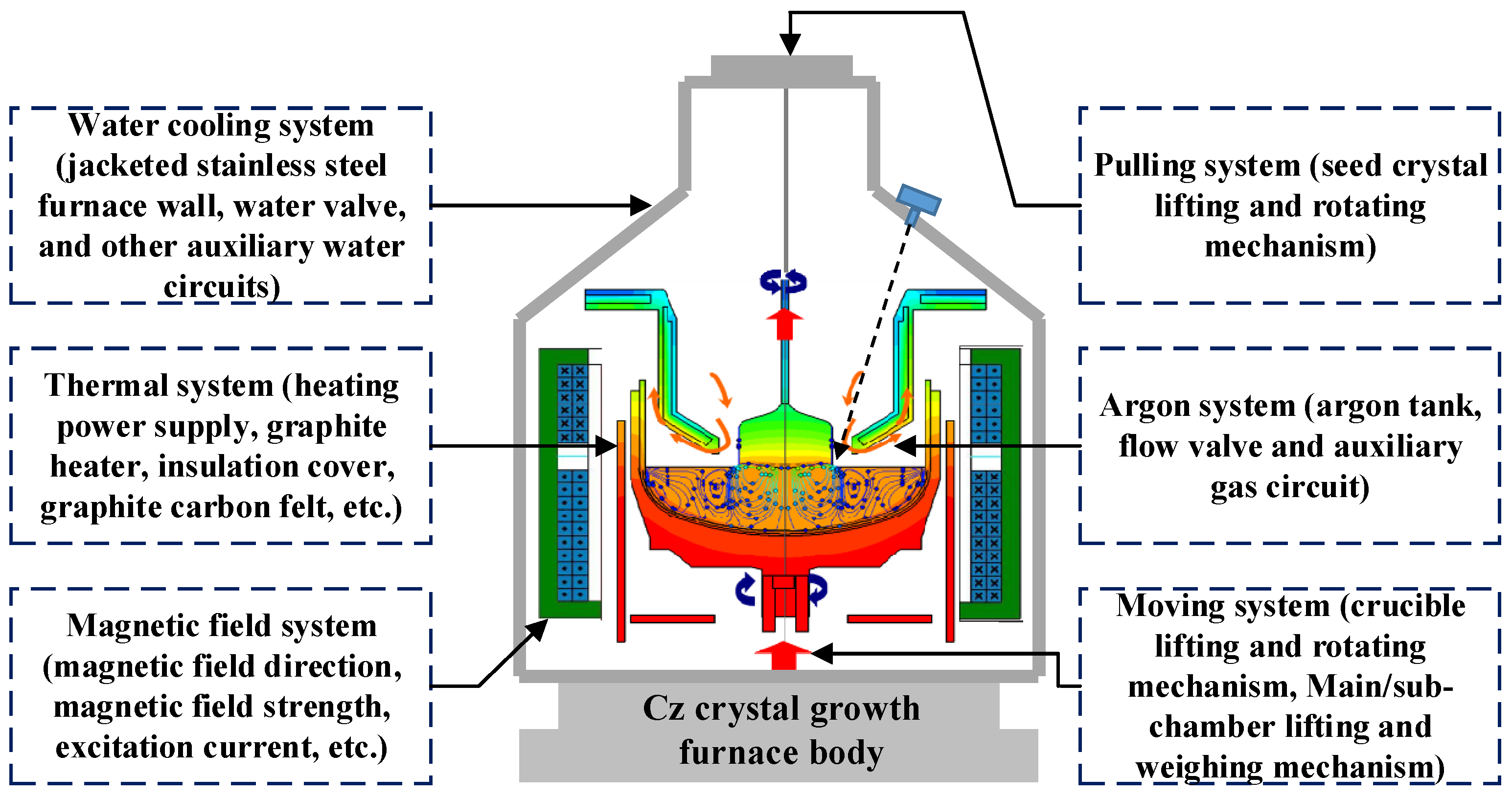
The Cz-SSC industry is a typical nonlinear dynamic process industry. The goal of Cz crystal growth operation is to grow high-quality silicon single crystal products with low production costs under the condition of the stable operation of the single crystal furnace. Figure 2 shows the crystal growth state inside the single crystal furnace, which involves the complex multi-field coupling relationship and the complex environment in the high temperature and closed furnace. Therefore, in such a complex furnace environment, efficiently, stably, and reliably realizing the growth process of high-quality SSC is very difficult.

At present, with the further narrowing of the integrated circuit linewidth, the native point defects in the crystal have an increasing impact on the performance of integrated circuit chips. The traditional macroscopic target (such as the crystal diameter or thermal field temperature) detection results have had difficulty reflecting the primary point defects inside the crystal, which is not conducive to the improvement of crystal quality. Therefore, understanding how to detect the crystal micro-quality index in real time during the Cz process has become an important research direction in the process control of high-quality semiconductor SSC. Based on this, Voronkov proposed the so-called “v/G criterion”, namely $v/G={\mathsf{\Gamma }}_{crit}$, in 1982. It can determine whether the primary point defects within the SSC are enriched with vacancies or self-interstitials. At the same time, Voronkov pointed out that a “v/G” of between 1 and $2.2\times {10}^{-3}$ (${\text{cm}}^2{\mathrm{K}}^{-1}{\min }^{-1}$) can grow perfect SSC. The “v/G criterion” points out that when $v/G>{\mathsf{\Gamma }}_{crit}$, the grown crystals are vacancy-rich, which leads to the appearance of “crystal source particles” and adversely affects the gate oxidation performance of the device. When $v/G<{\mathsf{\Gamma }}_{crit}$, the crystal is self-interstitial-enriched, which will produce dislocation clusters. When $v/G={\mathsf{\Gamma }}_{crit}$, the formed intrinsic point defect clusters are much smaller, which will not affect the performance of the back-end device.

Based on the above, in the process control of Cz-SSC, it is generally anticipated that the critical value ${\mathsf{\Gamma }}_{crit}$ of “v/G” is within the expected range. It can be clearly seen that the ${\mathsf{\Gamma }}_{crit}$ is directly associated with the crystal pulling rate and the axial temperature gradient. The mathematical relationship of the axial temperature gradient, $G$, is described as follows [6]:

$$G={\displaystyle \frac{T_{mel}-T^{*}}{h_{men}}}$$

(1)

where $T_{mel}$ indicates the melt temperature, $T^{*}$ indicates the melting point temperature, and $h_{men}$ is the height of the meniscus. However, in the actual industry, due to the limitations of physical structures and measurement technology, the meniscus height cannot be directly measured by hard sensors. To this end, ref. [16] showed an equation in which the meniscus height, $h_{men}$, is a function of the crystal radius, $r_{cry}$, and the crystal tilt angle, ${\alpha }_c$.

$$h_{men}=a\sqrt{{\displaystyle \frac{1-\sin ({\alpha }_0+{\alpha }_c)}{1+\frac{a}{\sqrt{2}{r}_{cry}}}}}$$

(2)

$$a=\sqrt{{\displaystyle \frac{2\gamma }{p_{mel}g}}}$$

(3)

$${\dot{r}}_{cry}=v\tan (\phi )$$

(4)

where ${\rho }_{mel}$ is the melt density, and $\gamma$ indicates surface tension. $g$ indicates the acceleration of gravity. ${\alpha }_0$ is the crystal growth angle, usually ${11}^0$.

According to the above Equations (1)–(4), it can be seen that the v/G value is related to the $v$, the $r_{cry}$, and the $T_{mel}$. However, in the Cz-SSC growth field, the crystal radius, $r_{cry}$, is obtained indirectly by CCD camera and image processing, and the melt temperature, $T_{mel}$, is obtained by non-contact infrared temperature sensors. Furthermore, there is a delay in obtaining the v/G value by the means of calculation, which is not conducive to real-time online control. More importantly, only the current v/G value can be obtained based on the above formula, and it is difficult to predict future trends. This will not be helpful to the on-site operator judging the future crystal quality change trend, thus causing them to fail to perform the correct crystal growth process adjustment action in time. Therefore, to solve these issues, understanding how to realize the soft sensor modeling of the difficult-to-measure crystal quality index v/G based on the easy-to-measure process variable data has become the focus of this paper. The results of this study can provide reliable and real-time crystal quality index v/G prediction data, assist field operators and control systems to make accurate control actions, and ensure the healthy growth of high-quality SSC.

2.2. v/G Prediction Strategy Design

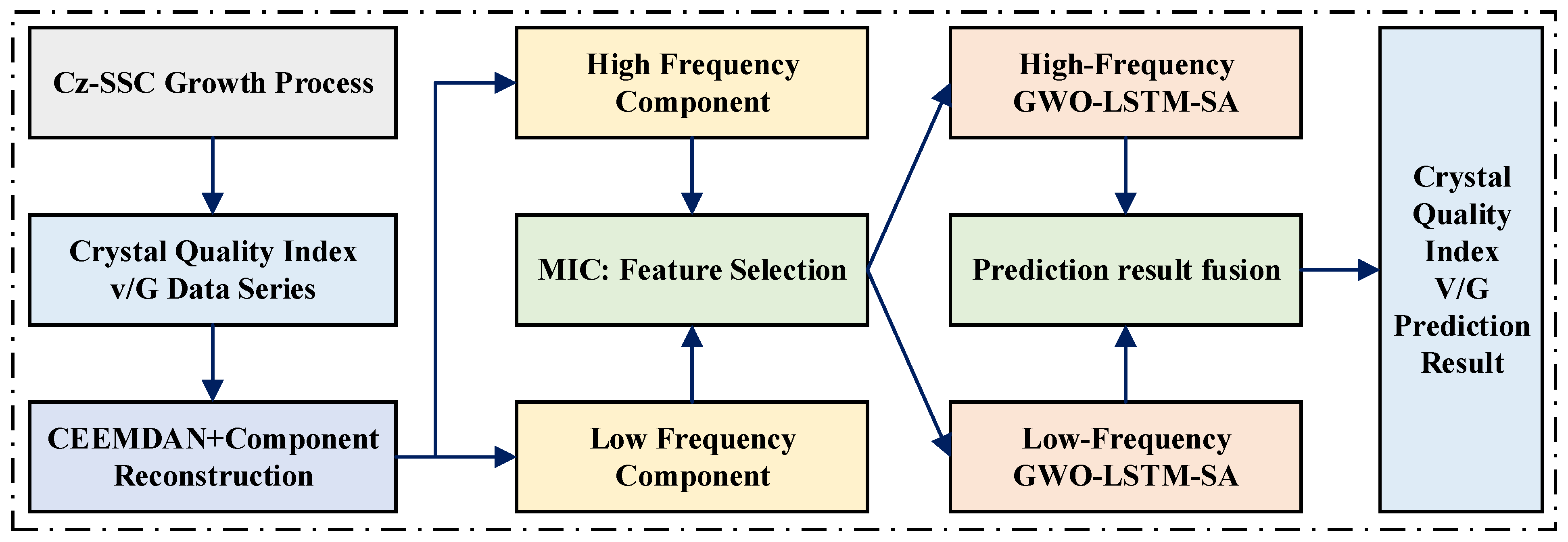
Considering that the existing data-driven v/G prediction methods mainly focus on the modeling of a single timescale, the prediction accuracy caused by the difference in the process variables in different time distributions is ignored. The crystal quality index v/G value is not only affected by other variables in Cz process but also by the previous v/G value. The previous v/G value affects the current v/G value on a short timescale, while other variables affect the current v/G value on multiple timescales. Therefore, in order to precisely predict the future v/G value, it is necessary to take into account the nonlinear and non-stationary characteristics of the v/G value data and the multi-timescale characteristics of influencing factors, so as to construct a data-driven v/G soft sensor prediction model, which will have a reliable application value in the control of the Cz-SSC growth process. Based on these analyses, this paper designs a scheme to predict the v/G index, as shown in Figure 3.

The model first uses the CEEMDAD decomposition method to decompose the v/G value time series step by step and then reconstructs the components according to the sample entropy of each component. At the same time, the timescale of each influencing factor is aligned with the timescale of the v/G value. Then, the correlation between the reconstructed components and the influencing factors is analyzed. According to the characteristics of different components and their influencing factors, The LSTM network prediction models with a self-attention mechanism are established sequentially, and the parameters of the prediction model are fine-tuned using the grey wolf optimization (GWO) algorithm. Finally, the predicted values of each component are fused to obtain the final crystal quality index v/G predicted value. It is worth noting that in the actual prediction process, the v/G values are predicted one by one, and the recursive prediction is carried out in combination with the feature quantity. When the number of prediction steps reaches a sliding step, the data sequence is decomposed again by sliding a step, and the components and features are incorporated into the prediction model in order to facilitate the continuation of the prediction process.

3. Soft Sensor Modeling Based on Multi-Timescale Feature Fusion

3.1. CEEMDAD Decomposition and Component Reconstruction

The crystal quality index v/G sequence contains multiple timescale components. It is an effective way to understand the characteristics of v/G by decomposing it into the sub-sequences of different timescales. The CEEMDAD can adaptively decompose signals based on the multi-timescale characteristics of signals and overcome the problem of modal aliasing in empirical mode decomposition and the problem of residual noise in decomposed signals [17]. Compared with ensemble empirical mode decomposition (EEMD) and complete ensemble empirical mode decomposition (CEEMD), CEEMDAD can improve the accuracy and stability of signal decomposition and has the highest decomposition efficiency [18]. Therefore, this paper uses the decomposition method based on CEEMDAD to decompose the crystal quality index v/G sequence into multiple components with different frequencies. The implementation steps of the CEEMDAD decomposition algorithm are as follows:

The white noise, $w^i(k)$($i=1,\cdots ,n$), and standard deviation, ${\epsilon }_0$, are added to the crystal quality index v/G data, $y(k)$, where $k$ is the sampling time.

$$y^i(k)=y(k)+{\epsilon }_0{w}^i(k)$$

(5)

The empirical mode decomposition (EMD) method is used to decompose $y^i(k)$, and then the decomposed components are averaged to calculate the first IMF, $im{y}_1(k)$, and the first residual, $r_1(k)$:

$$im{y}_1(k)={\displaystyle \frac{1}{n}}{\displaystyle {\sum }_{i=1}^{n}im{y}_1^i}(k)$$

(6)

$$r_1(k)=y(k)-im{y}_1(k)$$

(7)

Add the first residual $r_1(k)$. $r_1(k)+{\epsilon }_{1}EM{D}_1(w^i(k))$ can be decomposed by EMD to obtain $im{y}_2(k)$ and the second residual $r_2(k)$ of CEEMDAN, as shown in Equations (8) and (9):

$$im{y}_2(k)={\displaystyle \frac{1}{n}}{\displaystyle {\sum }_{i=1}^{n}EM{D}_1}(r_1(k)+{\epsilon }_{1}EM{D}_1(w^i(k)))$$

(8)

$$r_2(k)=r_1(k)-im{y}_2(k)$$

(9)

where $EM{D}_j$ is the $j$th IMF.

The calculation of the rest of the IMF is the same as step 3. Add new $w^i(k)$($i=1,\cdots ,n$) and ${\epsilon }_m$ to the new residual signal, as shown in Equations (10) and (11):

$$im{y}_k(t)={\displaystyle \frac{1}{n}}{\displaystyle {\sum }_{i=1}^{n}EM{D}_1}(r_{m-1}(k)+{\epsilon }_{m-1}EM{D}_{m-1}(w^i(k)))$$

(10)

$$r_m(t)=r_{m-1}(k)-im{y}_m(k)$$

(11)

where $m=2,3,\cdots ,M$. Here, $M$ denotes the sum of all the IMF components.

In instances where the number of residual extreme points does not exceed two, the CEEMDAN algorithm reaches a state of termination. Finally, the original crystal quality index v/G data $y(k)$ can be expressed as Equation (12):

$$y(k)=R(k)+{\displaystyle {\sum }_{m=1}^{M}im{y}_m}(k)$$

(12)

Figure 4 shows the 15 sub-sequences obtained by the CEEMDAD decomposition of the crystal quality index v/G sequence. The frequencies of the 15 sub-sequences are different, and the frequencies gradually decrease from IMF1 to IMF15, indicating that the crystal quality index v/G data sequence contains components of multiple timescales. Moreover, from the perspective of each component sequence, each has different degrees of the irregular change trend, and the fluctuation degree of the curve from IMF1 to IMF15 gradually decreases, indicating that the crystal quality index v/G data sequence is nonlinear and non-stationary.

Through the above CEEMDAD decomposition method, components of different frequencies can be obtained. However, for the crystal quality index v/G data sequence containing industrial noise, the CEEMDAD decomposition cannot fully deal with the influence of the noise on each component, and the proportion of the noise in each component is inconsistent, resulting in large differences in each component. It is evident that in order to enhance the efficacy and precision of predictions, the sample entropy must be utilized to assess the order magnitude of each constituent and to facilitate its reconstruction. Sample entropy can reflect the complexity of non-stationary signals. The large entropy value indicates that the disorder in the original signal is high and the characteristics of the noise signal are obvious. The small entropy value indicates that the trend and periodicity of the original signal are high. Therefore, the sample entropy is introduced to divide the threshold of the information component, and it is used as the criterion to distinguish the high-frequency component from the intermediate-frequency component and the low-frequency component across all the components, which can effectively identify the boundary of the v/G time series signal component.

Assuming that the time series of a component obtained by CEEMDAD decomposition is expressed as $Y=\{y_1,y_2,\cdots ,y_n\}$, it is reconstructed into the $d$-dimensional sequences $y_d(i)$ and $y_d(j)$. The distance between $y_d(i)$ and $y_d(j)$ is calculated by Equation (13), and the number of $B(i)$ whose distance is less than the threshold, $\gamma$, is counted. Then, the ratio $B^d(\gamma )$ is calculated by Equations (14) and (15), and the dimension of the sequence is extended from $d$ to $d+1$. Repeat the above steps, replace $d$ in Equations (13) and (14) with $d+1$, and calculate $B_i^{d+1}(\gamma )$. Finally, $B^{d+1}(\gamma )$ is obtained by Equation (16), and then the sample entropy, $SE$, can be obtained by Equation (17). The specific calculation method is as follows [19]:

$$D_d(Y_i,Y_j)=\max \left\{\left|y_d(i),y_d(j)\right|\right\}$$

(13)

$$B_i^d(\gamma )={\displaystyle \frac{1}{M-d}}B(i)$$

(14)

$$B^d(\gamma )={\displaystyle \frac{1}{M-d+1}}{\displaystyle \sum _{i=1}^{M-d+1}{B}_i^d(\gamma )}$$

(15)

$$B^{d+1}(\gamma )={\displaystyle \frac{1}{M-d}}{\displaystyle \sum _{i=1}^{M-d}{B}_i^{d+1}(\gamma )}$$

(16)

$$SE(d,\gamma ,M)=-\ln \left({\displaystyle \frac{B^{d+1}(\gamma )}{B^d(\gamma )}}\right)$$

(17)

According to the above calculation results, the sample entropy values shown in

Table 1. The sample entropy (SE) values of different components.

Component	IMF1	IMF2	IMF3	IMF4	IMF5	IMF6	IMF7	IMF8
SE value	2.32	1.43	2.69	2.08	1.28	0.86	0.73	0.67
Component	IMF9	IMF10	IMF11	IMF12	IMF13	IMF14	IMF15	----
SE value	0.60	0.41	0.22	0.23	0.01	0.004	0.0003	----

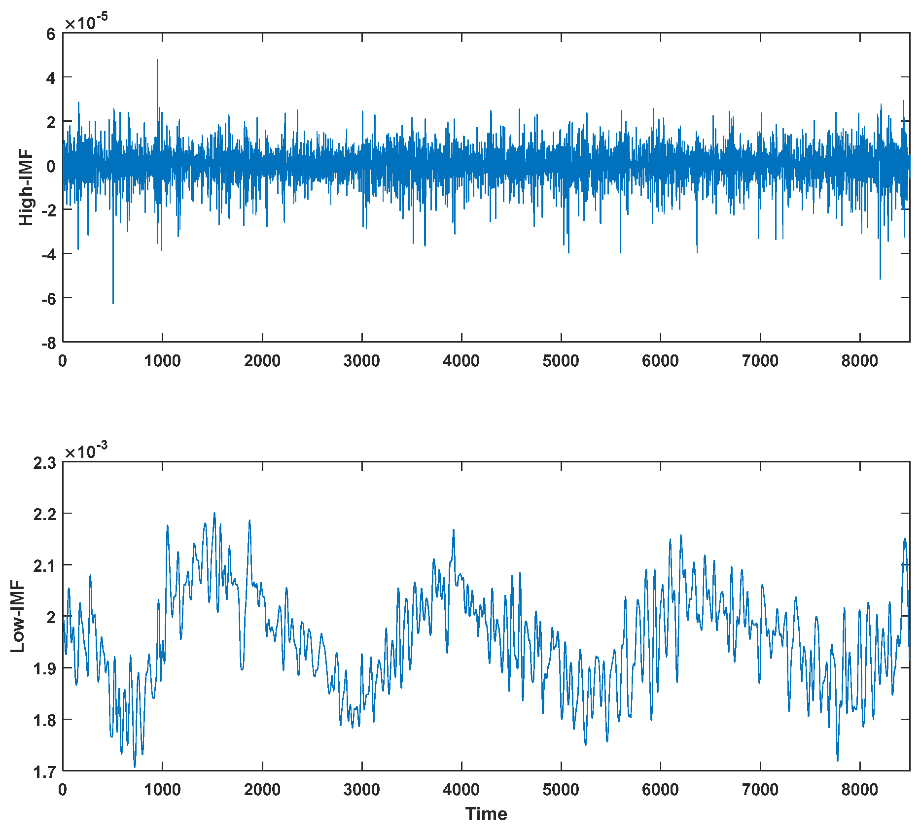
can be obtained. Figure 5 shows the reconstruction components. Here, the components with a sample entropy value of higher than 1 are summed as the high-frequency sequence, and the components with a sample entropy value of lower than 1 are summed as the low-frequency sequence. The high-frequency sequence has the characteristics of a short fluctuation period and a high frequency. Compared with the high-frequency sequence, the frequency of the low-frequency sequence decreases, with regular and periodic fluctuations. The low-frequency sequence reflects the long-term trend change in the v/G data sequence of the crystal quality index.

3.2. MIC-Based Feature Variable Selection

In the actual Cz-SSC growth process, there are many characteristic variables that affect the change in the crystal quality index v/G. Therefore, understanding how to select the most representative characteristic variables to reduce the complexity of the subsequent model construction and improve the modeling accuracy is very important. Therefore, in order to quantitatively describe the degree of correlation between the process variables and the crystal quality index v/G, this paper uses the MIC as a feature variable selection method [20]. In comparison with mutual information, the MIC has been shown to exhibit higher levels of accuracy and is considered to be an excellent method for the calculation of data correlation. The advantage of the MIC lies in its universality and balance, and it is a more reliable analysis method in statistical analysis.

The concept of mutual information is explained by the following equation:

$$I(X,Y)={\displaystyle \sum _{x\in X}{\displaystyle \sum _{y\in Y}p(x_i,y_j)}}{\log }_2{\displaystyle \frac{p(x_i,y_j)}{p(x_i)p(y_j)}}$$

(18)

where $p(x_i,y_j)$ is the joint probability of variable $x_i$ and target variable $y_j$. $p(x_i)$ and $p(x_j)$ represent the marginal distribution probabilities of the $i$th variable $x_i$ and the $j$th target variable $y_j$, respectively.

The concept of the MIC involves discretizing the relationship between variables $X$ and $Y$ in a 2D space, represented through a scatter plot, $G_{<x_i,y_j>}$. Then, the current 2D space is divided into certain interval numbers in any $<x_i,y_j>$ direction. Next, we examine the scatter points currently present in each square, representing the calculation of the joint probability. The following gives the calculation formula of the MIC:

$$MI{C}_{<x_i,y_j>}=\underset{x_i,y_j<B(n)}{\max }\left\{{\displaystyle \frac{I(X,Y){|}_{G_{<x_i,y_j>}}}{{\log }_2\min (x_i,y_j)}}\right\}$$

(19)

where $B(n)$ is a function of the number of samples, $n$. In general, when $B(n)=n^{0.6}$, the MIC works well in practice. A higher MIC value indicates a stronger correlation between the two variables.

A large amount of detection data that can reflect the crystal growth state are recorded in the historical database of the Cz silicon single crystal furnace. According to the crystal growth process mechanism of the Cz silicon single crystal furnace, the installed sensor detection equipment, and the field expert experience, the process variable factors that affect the prediction of the crystal quality index v/G are preliminarily determined, as shown in

Table 2. Description of different process variables.

Variable	Description	Variable	Description
$x_1$	Heater power	$x_8$	Argon flow rate
$x_2$	Thermal field temperature	$x_9$	Crystal length
$x_3$	Pulling speed	$x_{10}$	Liquid level position
$x_4$	Crystal rotation speed	$x_{11}$	Crystal diameter
$x_5$	Crucible lifting speed	$x_{12}$	Furnace pressure
$x_6$	Crucible rotation speed	$y$	v/G value
$x_7$	Crystal weight	---	---

.

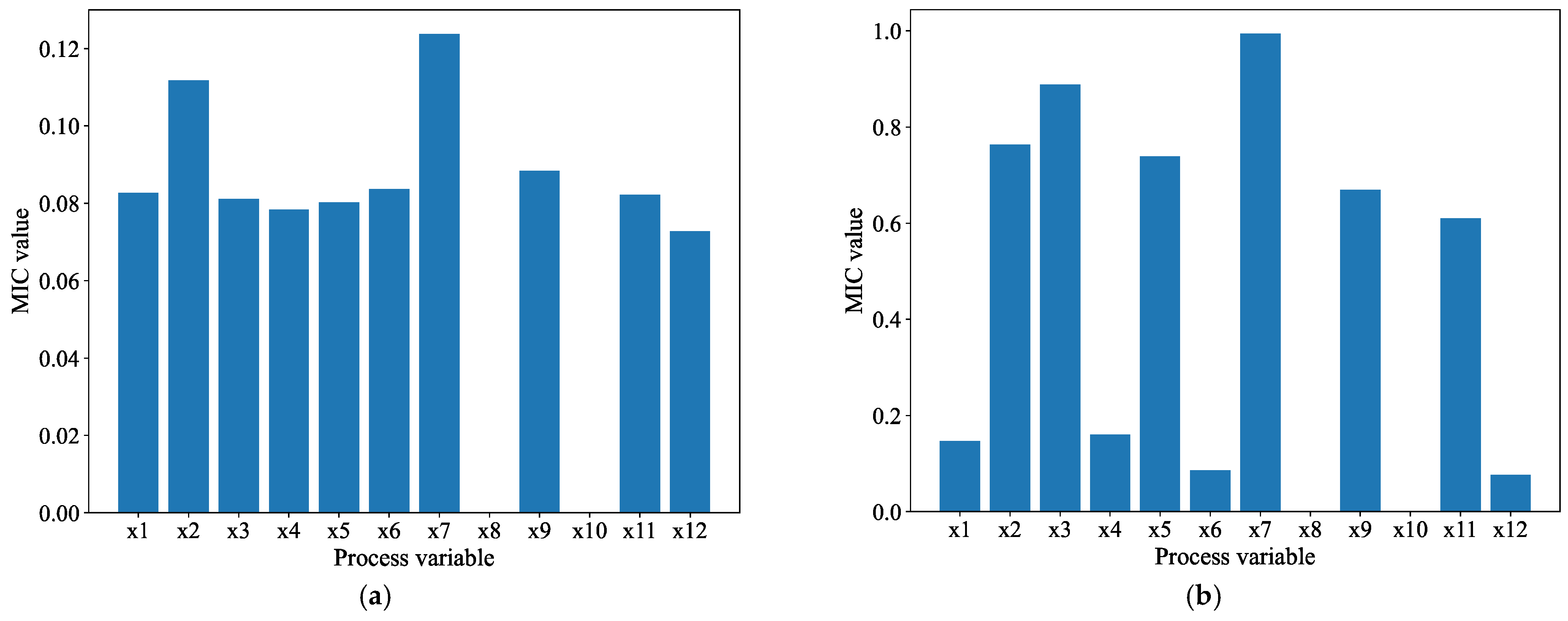
In order to quantitatively describe the correlation between the process variables selected by the expert’s experience, shown in Table 2, and the crystal quality index v/G reconstruction component, the above the MIC method is used to calculate the correlation between the two variables, as shown in Figure 6a,b. Specifically, Figure 6 shows the correlation between the MIC coefficients of the high-frequency components, the low-frequency components, and the influencing factors, respectively.

According to Figure 6a, except for $x_8$ and $x_{10}$, the other process variables have a great influence on the high-frequency component of the v/G. In Figure 6b, compared with the other process variables, $x_2$, $x_3$, $x_5$, $x_7$, $x_9$, and $x_{11}$ have a greater impact on the low-frequency component of the v/G. Therefore, the high-frequency sequence selects $x_1\sim x_7$, $x_9$, $x_{11}$, and $x_{12}$ as the input of the prediction model, and the low-frequency sequence selects $x_2$, $x_3$, $x_5$, $x_7$, $x_9$, and $x_{11}$ as the input.

3.3. Long Short-Term Memory Network Based on SA

(1)

Standard long short-term memory network (LSTM)

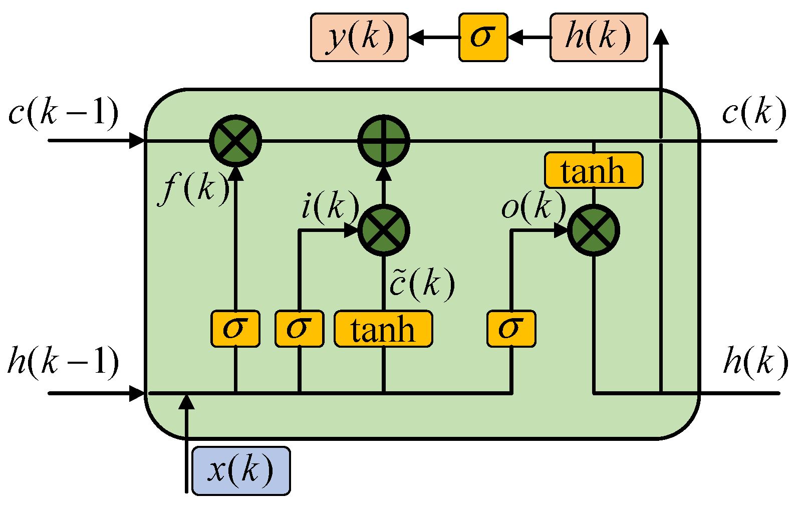
LSTM is a special form of a recurrent neural network (RNN). It is capable of capturing long-term dependencies and is well-suited for handling significant events with extended intervals and delays in time-related data sequences. It is often used for nonlinear prediction modeling [21,22]. The outstanding feature of LSTM is the use of a gate structure to regulate the flow of information. The gate determines which data are crucial for memory or forgetting, allowing the relevant information to be transmitted along the long sequence chain so that it can make accurate predictions. The standard LSTM network has three main gates, namely, the forgetting gate, the input gate, and the output gate. The forgetting gate regulates which state information from the previous unit should be kept or discarded in the current unit’s state, while the input gate decides the amount of new information to be added to the cell state. The output gate determines whether the current value in the adjustment unit contributes to the output. The structure of the LSTM with these three gates is illustrated in Figure 7.

In Figure 7, LSTM includes the input gate, forgetting gate, internal state update, and output gate. The basic update rules of the LSTM network in a unit can be expressed as follows:

(1)

Input gate:

$$i_k=\sigma \left(W_{xi}{x}_k+W_{hi}{h}_{k-1}+b_i\right)$$

(20)

where $i_k$ is the output of the input gate, $x_k$ is the current input value, and $h_{k-1}$ is the output value of the previous moment. $W_i$ and $W_{hi}$ are the input gate weight matrix and the recursive weight matrix, respectively. $b_i$ is the input gate bias, and $\sigma (\cdot )$ is the sigmoid function.

(2)

Forgetting gate:

$$f_k=\sigma \left(W_f{x}_k+W_{hf}{h}_{k-1}+b_f\right)$$

(21)

where $f_k$ is the output, $W_f$ and $W_{hf}$ are the weight matrix and the recursive weight matrix, respectively, and $b_f$ is the offset of the forgetting gate.

(3)

Internal unit state update:

$$c_k=f_k\times c_{k-1}+i_k\times \tanh (W_c{x}_k+W_{hc}{h}_{k-1}+b_c)$$

(22)

where $c_k$ and $c_{\mathrm{k}-1}$ are the current internal unit state and the internal unit state at the previous moment, $W_c$ and $W_{hc}$ are the internal unit state weight matrix and the recursive weight matrix, and $b_c$ is the bias of the internal unit state.

(4)

Output gate:

$$o_k=\sigma (W_o{x}_k+W_{ho}{h}_{k-1}+b_o)$$

(23)

$$h_k=o_k·\tanh (c_k)$$

(24)

where $o_k$ is the output of the output gate, $W_o$ and $W_{ho}$ are the output gate weight matrix and the recursive weight matrix, respectively, and $b_o$ is the bias.

(2)

Self-attention mechanism (SA)

SA is a resource allocation mechanism that mimics the human brain. The SA mechanism is a special attention mechanism that allows the model to consider the relationship between each element in the sequence and all other elements when dealing with a sequence [23,24]. This mechanism is particularly effective in capturing the internal correlation of data and also reduces the need for external information. Figure 8 shows the structure of the self-attention mechanism, which is mainly composed of three vectors: query (q), key (k), and value (v). For a query, the attention mechanism calculates the similarity between the query and the keyword and assigns higher weights to the values with high similarity.

Define the query vector as $Q={[q_1,q_2.\cdots ,q_L]}^T$, the key vector as $K={[k_1,k_2.\cdots ,k_L]}^T$, and the value vector as $V={[v_1,v_2.\cdots ,v_L]}^T$, where L is the time step. The calculation formula of SA is as follows:

$$Attention(Q,K,V)=softmax\left({\displaystyle \frac{Q{K}^T}{\sqrt{d_k}}}\right)V$$

(25)

where the softmax function applies normalization to the attention score. $d_k$ is the scale factor. Equation (25) determines the weight distribution of the value by the similarity between the query and the key, so as to obtain the attention score. These attention scores determine the weight of each sample in the sequence and give higher weights to more relevant entities.

In summary, SA is a mechanism for allocating weight parameters aimed at helping the model capture critical information. Specifically, given a set of <key, value> pairs and a target vector (query), the SA mechanism calculates the similarity between the query and each key, determines the weight coefficients for the keys, and computes the final attention value by summing the weighted values.

(3)

SA-based LSTM model

It is well known that the introduction of the advantages of deep network modeling has improved the accuracy of the prediction of the key performance indicators of industrial processes. However, there are still some problems in directly establishing the online prediction model of the crystal quality index v/G based on the LSTM deep network. Firstly, the trained LSTM network will extract the abstract feature representation of each dimension process variable of the input sample indiscriminately to complete the crystal quality index v/G prediction task. In fact, for the Cz-SSC growth process, especially when the operating conditions change frequently, the importance of the process variables affecting the crystal quality index v/G presents a dynamic change rule. Therefore, the modeling idea of using only the conventional LSTM network cannot fully describe the dynamic Cz-SSC process. In addition, the conventional LSTM network has difficulty focusing on the importance of the input process variables. Therefore, to address the above issues and enhance the prediction accuracy of the crystal quality index v/G, we integrated the SA mechanism with the LSTM (referred to as LSTM-SA) and leveraged SA to strengthen the LSTM network. In short, the introduction of the self-attention mechanism has enabled the handling of features on different timescales, which is crucial for capturing the dynamics and temporal relationships of the crystal quality index v/G as they evolve over time.

The LSTM-SA architecture is depicted in Figure 9. The LSTM-SA network model consists of five layers: an input layer, an LSTM layer, an SA layer, a fully connected layer, and an output layer. The input layer feeds sample data points into the model. The LSTM layer processes the input data using a long short-term memory hidden layer, converting it into high-level abstract features. The SA layer computes a weight vector, emphasizing the more significant weights in the hidden state information, and applies weighting to all hidden states of subsequent time steps. In the fully connected layer, every neuron is linked to all the neurons in the preceding layer to facilitate the information exchange between them. The output layer utilizes feature vectors to predict the time series data. It is worth noting that in the LSTM-SA network structure, the SA mechanism module is embedded in the back end of the deep LSTM network to calculate the attention score of each process variable of the input sample in real time after passing through the LSTM layer, so as to give a higher weight to the key part of the input data. Thus, the accuracy of the prediction is improved.

In summary, integrating the SA mechanism into the LSTM network helps to mine credible and clear relationships between the variables, so that we can use the production data to make accurate crystal quality index v/G predictions. For the Cz-SSC growth process, there are many process variables that affect the crystal quality index v/G, and it is difficult for the conventional LSTM network to focus on the process variables that have a greater impact on the v/G index from these variables, so the v/G prediction accuracy will be degraded over time. Although the LSTM network works well when dealing with long-term sequence data, when it is integrated with the SA mechanism, even if the data has noise, it can adjust the input importance at different times by learning dynamic weights, making the model pay more attention to the process variables of the key time points required for v/G prediction, so as to predict the target variables more accurately.

3.4. The Hyperparameters of the LSTM-SA Model Are Optimized Based on GWO

It is well known that the performance of the above LSTM-SA network depends on the setting of multiple network parameters. Among them, the number of unit layers, the number of hidden nodes, the learning rate, and the batch scale parameters of the LSTM network have the greatest impact on the model performance. Therefore, in order to avoid the time-consuming cost of manually adjusting network parameters, this paper uses the grey wolf optimization (GWO) algorithm to optimize the above four parameters. The GWO algorithm has the advantages of global convergence and a fast convergence speed [25], which can ensure that the LSTM-SA model can converge to the global optimum.

The optimization goal of the LSTM-SA network parameters based on GWO is to make the predicted value of the model as close as possible to the actual value. In other words, the objective function is to minimize $g(y,\widehat{y})={\displaystyle \frac{1}{N}}{\displaystyle {\sum }_{k=1}^N{(y_k-{\widehat{y}}_k)}^2}$. $\widehat{y}$ is the predicted value, and $y$ is the actual value. The fitness function of the GWO algorithm can be set to

$$fitness={\displaystyle \frac{1}{N}}{\displaystyle {\sum }_{k=1}^N{(y_k-{\widehat{y}}_k)}^2}$$

(26)

The GWO algorithm determines the optimal parameters for the LSTM-SA network model by calculating Equation (26) and updating the positions of the wolf pack. These optimal parameters are then used to build a v/G prediction model for the crystal quality indicator. The flow of the crystal quality indicator v/G prediction model based on GWO-based LSTM-SA (called GWO-LSTM-SA), proposed in Figure 10.

Step 1: The function of the data preprocessing module is to eliminate outliers, add missing values, and normalize the data with respect to the crystal quality index v/G and the sample data of the process variables collected by the Cz-SSC growth control platform. Afterwards, the cleaned dataset is divided into a training set and a test set.

Step 2: GWO initialization, including the number of gray wolf populations, the number of iterations, and the upper and lower bounds of the parameters to be optimized. The to-be-optimized parameters of the LSTM-SA network are converted to the position coordinates of the wolf population, and the training sample set is selected to train the model of LSTM-SA.

Step 3: Calculate the wolf pack individual fitness value; the grey wolf fitness function is set to the above Equation (26). It is evident that the smaller the fitness function value, the more it is preferable. Update the wolf pack individual position according to the fitness value. The optimal solution for the number of LSTM layers, hidden nodes, learning rate, and batch scale parameter of the LSTM-SA network is achieved when the search reaches the maximum iterations or the global optimal position.

Step 4: The optimal GWO-LSTM-SA network model obtained is tested on the sample set to predict the crystal quality index v/G.

4. Cz-SSC Growth Process Simulation Experiment and Result Analysis

4.1. Data Set Description and Pre-Processing

To verify the effectiveness of the method proposed in this paper, 8300 sets of sample data were selected from the 12-inch Cz-SSC growth, with a sampling time of 2 s. In some scenarios, the data collected during the experimental process will be erroneous due to the failure of the sensor equipment or the computer entry error, etc., and also the interference of the onsite Cz-SSC process may make a lot of noise appear in the measurement data. Therefore, before modeling, the data need to be preprocessed to obtain standard, clean, and continuous data for the subsequent modeling.

The abnormal data caused by a sensor equipment failure or computer input error are directly eliminated by the $3\sigma$ criterion. Regarding the noise in the data, it is processed by mean filtering. There are large differences in the dimensions of different process variables for the samples in the dataset. Therefore, it is necessary to standardize the data before modeling to eliminate the influence of the different dimensions on the model. In this paper, Equation (27) is used to normalize the data.

$${\widehat{x}}_i={\displaystyle \frac{x_i-\overline{x}}{x_{\max }-x_{\min }}}$$

(27)

where ${\widehat{x}}_i$ is the result of the standardization of the $i$th process variable. $x_{\max }$ and $x_{\min }$ are the maximum and minimum values of the $i$th process variable sample, respectively.

For each component sequence obtained by CEEMDAN decomposition, the first 70% of the data is used for model training, 20% of the data is employed for the testing of the model, and the final 10% of the data is allocated for the verification of the model.

4.2. Evaluation of Model Prediction Performance

To assess the predictive capacity of the model, the discrepancy between the modeled values and the observed values is quantifiable by the mean absolute error (MAE) and the root mean square error (RMSE). The MAE and RMSE are defined as follows:

$$MAE={\displaystyle \frac{1}{N}}{\displaystyle {\sum }_{k=1}^N\left|y_k-{\widehat{y}}_k\right|}$$

(28)

$$RMSE=\sqrt{{\displaystyle \frac{1}{N}}{\displaystyle {\sum }_{k=1}^N{(y_k-{\widehat{y}}_k)}^2}}$$

(29)

where $y_k$ represents the actual observed value and ${\widehat{y}}_k$ represents the predicted value of the model. $N$ is the number of samples. The smaller the statistical indicators MAE and RMSE are, the better the performance of the model. It is the considered opinion of experts that the absolute value of the error between the predicted value and the actual observed value within the range of $0.15\times {10}^{-4}$ is an acceptable result, which is more conducive to ensuring that the crystal quality meets the standard. In order to show the prediction effect of the model more intuitively, the prediction hit rate of the model is defined as

$$HR={\displaystyle \frac{1}{N}}{\displaystyle \sum _{k=1}^N(H(k))}\times 100\%$$

(30)

where $H(k)$ is the Heaviside function of the k-th sample [26], defined as

$$H(k)=\{\begin{array}{l}1, \left|y_k-{\widehat{y}}_k\right|\le 0.15\times {10}^{-4}\\ 0, otherwise\end{array}$$

(31)

4.3. Crystal Quality v/G Index Simulation Prediction Results and Analysis

In order to better demonstrate the detailed fitting of the predicted values to the actual values, Figure 11 only shows the prediction result of the validation set, and Figure 11a–c show the prediction effect of the high-frequency component, the low-frequency component, and the fused v/G, respectively. Here, the parameters of the prediction model optimized by GWO are set as follows: the quantity of neurons in the hidden layer of the neural network, the amount of network unit layers, the learning rate, and the batch scale parameter of the high-frequency component LSTM-SA model are 34, 3, 0.005, and 30, respectively. The quantity of neurons in the hidden layer of the neural network, the quantity of network unit layers, the learning rate, and the batch scale parameter of the low-frequency component LSTM-SA model are 73, 1, 0.0089, and 74. The training process of all the models was done in the deep learning framework PyTorch 2.1 with a computer CPU of intel(R) Core(TM) i9-14900KF with 3.20 GHz and 32 GB of RAM.

From the above prediction effect of each component, it can be seen that the model is able to effectively predict each component, and the actual value of the v/G can be accurately predicted by fusing the prediction results of the high-frequency and low-frequency sequences, as shown in Figure 11c. Although the overall prediction performance of the v/G is good, the prediction accuracy of the peaks and valleys of some components is relatively low, which is mainly due to the fact that the very high or very low v/G values are usually closely related to the abnormal working conditions of the Cz process, and thus the predictability is poor.

Table 3. Comparison of predictive performance indexes of different components of v/G.

v/G Component	MAE	RMSE	HR
$y_h$	4.80 × 10−6	6.76 × 10−6	88.64%
$y_l$	4.46 × 10−6	5.44 × 10−6	99.64%
$y$	6.34 × 10−6	8.48 × 10−6	92.53%

gives a comparison of the prediction performance metrics for the high-frequency component, low-frequency component, and fusion sequences of the v/G. $y_h$ and $y_l$ represent the high-frequency component sequences and low-frequency component sequences, respectively. The evaluation metrics, the MAE and the RMSE, of the low-frequency component are lower than those of the high-frequency component, and the hit rate HR is higher, which indicates that the low-frequency sequence is better fitted. The evaluation metrics for the high-frequency components, i.e., the higher MAE and RMSE and the lower HR, are consistent with the fact that the high-frequency components fluctuate on a larger scale and are not easy to predict. It is because of the fluctuating characteristics of the high-frequency component that the fused v/G prediction performance index is weaker than that of the low-frequency component.

To validate the effectiveness of the proposed prediction model, comparisons were made with other prediction models based on the following criteria. In order to test the difference in the prediction performance between the decomposition fusion model and the single model, a single SVM model, LSTM model, and LSTM-SA prediction model were introduced for comparison. According to the results shown in Figure 12, the single-timescale prediction is not as accurate as the multi-timescale prediction. It can only roughly follow the trend of the expected output, ignoring the detailed information of the v/G. Compared with other models, the proposed model has a higher accuracy in both the prediction value and the direction, and the numerical discrepancy is smaller. At the same time, the prediction results of the proposed model have a more consistent upward or downward trend with the actual values. The comprehensive comparison results further verify that the prediction accuracy of the multi-timescale prediction model is better.

To facilitate a more comprehensive comparison of the prediction performance of different models,

Table 4. The prediction performance of each model for v/G under three evaluation indexes.

Model	MAE	RMSE	HR
SVM	2.84 × 10−5	3.10 × 10−5	15.66%
LSTM	9.11 × 10−6	1.12 × 10−5	84.22%
LSTM-SA	7.82 × 10−6	9.92 × 10−6	88.31%
Proposed	6.34 × 10−6	8.48 × 10−6	92.53%

shows the prediction performance evaluation indexes. The evaluation indexes, the MAE and the RMSE, of the three single prediction models are larger than those of the proposed models. Among them, the evaluation indexes of the SVM are worse than the other models. Compared with the LSTM-SA model, the MAE and the RMSE indexes of the proposed model are reduced by 18.9% and 14.5%, respectively, while the HR index is increased by 4.8%. This result further verifies the effectiveness of the proposed multi-timescale fusion model.

4.4. Discussion of Simulation Results

In our study, the proposed deep learning model based on multi-timescale feature fusion combines LSTM and a self-attention mechanism to effectively capture the long-term dependencies and the feature importance in time series data. This gives our method a clear advantage in dealing with crystal quality metric v/G prediction, especially in complex industrial process data that are difficult to handle using traditional methods (e.g., SVM and LSTM). Compared with the existing methods, the model proposed in this paper not only improves the prediction accuracy but also demonstrates a better stability and generalization ability on different datasets. At the same time, this method is able to better portray and predict the trend of the crystal quality index v/G by integrating different timescale features, thus providing guidance to field operators and assisting the control system to make accurate control actions.

In general, it can be seen that for complex industrial process objects such as Cz-SSC, the deep learning prediction method based on data-driven crystal quality variables will become the current and future research hotspot. Although the method proposed in this paper shows its effectiveness in simulation experiments, it still has some limitations. In particular, in a highly noisy data environment, the model may be disturbed to some extent, leading to a decrease in the prediction accuracy. Future research can focus on how to further improve the robustness and adaptability of the model through data augmentation, optimal feature selection, or improved training strategies. In addition, the combination of other deep learning techniques or the fusion of multimodal data will potentially further improve the performance of the model in real industrial applications.

5. Conclusions

In this paper, considering the nonlinear, non-stationary, and multi-timescale characteristics of the v/G index in the growth process of Cz-SSC, an integrated learning soft sensor prediction model of the crystal quality index v/G that integrates multi-timescale characteristics was proposed. Firstly, CEEMDAD was used to decompose the v/G data sequence, and then each component was reconstructed according to the sample entropy. Based on this, the characteristic variables closely related to the reconstructed component were selected by the MIC. Then, an LSTM network prediction model based on an attention mechanism was established for the time feature components of different scales. Finally, by ensemble learning the predicted values of each sub-sequence component, the crystal quality index v/G prediction results with multi-timescale features were obtained. The effectiveness of the proposed soft sensor method was verified through simulation comparison experiments. In future research, considering the change in working conditions under the repeated operation, the transfer learning problem of the crystal quality index v/G should be studied and applied to the actual growth control process of Cz-SSC, which will provide guidance for the optimization of the high-quality silicon single crystal growth process. In summary, the proposed prediction model has the capacity to function as a soft sensor, thereby providing real-time crystal quality index v/G prediction information for the actual Cz-SSC production process, so as to make reasonable decisions for the optimization of single crystal furnace operation.