Abstract
Economic performance in modern manufacturing enterprises is often influenced by random dynamic events, requiring real-time scheduling to manage multiple conflicting production objectives simultaneously. However, traditional scheduling methods often fall short due to their limited responsiveness in dynamic environments. To address this challenge, this paper proposes an innovative online rescheduling framework called the Dual-Level Integrated Deep Q-Network (DLIDQN). This framework is designed to solve the dynamic multi-objective flexible job shop scheduling problem (DMOFJSP), which is affected by six types of dynamic events: new job insertion, job operation modification, job deletion, machine addition, machine tool replacement, and machine breakdown. The optimization focuses on three key objectives: minimizing makespan, maximizing average machine utilization (), and minimizing average job tardiness rate (). The DLIDQN framework leverages a hierarchical reinforcement learning approach and consists of two integrated IDQN-based agents. The high-level IDQN serves as the decision-maker during rescheduling, implementing dual-level decision-making by dynamically selecting optimization objectives based on the current system state and guiding the low-level IDQN’s actions. To meet diverse optimization requirements, two reward mechanisms are designed, focusing on job tardiness and machine utilization, respectively. The low-level IDQN acts as the executor, selecting the best scheduling rules to achieve the optimization goals determined by the high-level agent. To improve scheduling adaptability, nine composite scheduling rules are introduced, enabling the low-level IDQN to flexibly choose strategies for job sequencing and machine assignment, effectively addressing both sub-tasks to achieve optimal scheduling performance. Additionally, a local search algorithm is incorporated to further enhance efficiency by optimizing idle time between jobs. The numerical experimental results show that in 27 test scenarios, the DLIDQN framework consistently outperforms all proposed composite scheduling rules in terms of makespan, surpasses the widely used single scheduling rules in 26 instances, and always exceeds other reinforcement learning-based methods. Regarding the metric, the framework demonstrates superiority in 21 instances over all composite scheduling rules and maintains a consistent advantage over single scheduling rules and other RL-based strategies. For the metric, DLIDQN outperforms composite and single scheduling rules in 20 instances and surpasses other RL-based methods in 25 instances. Specifically, compared to the baseline methods, our model achieves maximum performance improvements of approximately 37%, 34%, and 30% for the three objectives, respectively. These results validate the robustness and adaptability of the proposed framework in dynamic manufacturing environments and highlight its significant potential to enhance scheduling efficiency and economic benefits.
1. Introduction
The flexible job shop scheduling problem (FJSP) is a common challenge in production scheduling and extends the classical job shop scheduling problem (JSP). JSP is a combinatorial optimization problem (COP) that is NP-hard [1]. In JSP, each job consists of a series of operations, with each operation assigned to a specific machine. In contrast, FJSP introduces a machine selection mechanism, allowing each operation to be assigned to any machine from a set of compatible options, increasing scheduling flexibility and complexity.
Most research on FJSP focuses on static production environments. However, real-world production is often uncertain, with dynamic events such as order changes, machine breakdowns, and task adjustments being unavoidable [2]. These disruptions can cause deviations from the original plan, rendering existing schedules ineffective and negatively impacting production efficiency and resource utilization. As a result, developing dynamic scheduling methods for multi-objective FJSP is crucial. These methods not only enhance theoretical models and algorithms but also offer significant practical value.
In practical manufacturing environments, dynamic real-time scheduling methods help manage uncertainty by improving system flexibility and robustness. They allow quick adjustments to job sequences and resource allocations, minimizing the impact of disruptions like machine breakdowns or order changes. Real-time scheduling optimizes multiple objectives, such as minimizing makespan, maximizing machine utilization, and reducing job tardiness. This multi-objective optimization improves efficiency, balances resource use, and ensures smooth operation despite dynamic disturbances.
Moreover, real-time scheduling supports continuous decision-making in highly automated production environments. It allows systems to quickly respond to changing conditions, reducing the need for human intervention and decision delays. This enhances operational efficiency and stability. In smart manufacturing, real-time scheduling helps businesses quickly recover from disruptions, improving customer satisfaction while boosting competitiveness, efficiency, and resource utilization.
The dynamic multi-objective flexible job shop scheduling problem (DMOFJSP) has been extensively studied in recent years, with numerous solutions emerging from years of exploration. Traditional methods for solving DMOFJSP generally fall into two categories: meta-heuristic algorithms and dispatching rules [3]. Meta-heuristic methods encompass a variety of algorithms, such as genetic algorithms (GA) [4,5], particle swarm optimization (PSO) [6], simulated annealing (SA) [7], grey wolf optimization (GWO) [8], ant colony optimization (ACO) [9,10], and tabu search (TS) [11]. These methods typically decompose dynamic scheduling problems into a series of static sub-problems, which are then solved sequentially. Although these methods can generate solutions close to the global optimum, their high computational complexity necessitates recalculating an optimal solution whenever a dynamic event occurs. This often results in prolonged computation times, hindering quick responses to dynamic changes and limiting their suitability for real-time scheduling.
Dispatching rules are widely used in dynamic job shop scheduling, where they prioritize jobs and machines based on specific criteria to allocate and process jobs. Known for their computational efficiency and simplicity, these rules are highly responsive in dynamic environments. However, many dispatching rules have limitations, often being too myopic to yield optimal long-term results [12]. In different shop configurations, no single dispatching rule consistently outperforms others [13,14]. A promising approach to balance time efficiency and solution quality involves dynamically selecting the most appropriate rule at each decision point. This enables short-term optimization of multiple objectives, ensuring timely scheduling while improving overall shop efficiency.
To select the most appropriate rule at each scheduling decision point, the DMOFJSP can be modeled as a Markov Decision Process (MDP), providing a formal framework for decision-making under uncertainty. In this framework, an intelligent agent chooses the optimal action from the action space based on the current state features of the environment. This involves selecting from predefined scheduling rules to optimize the scheduling objectives. Recently, reinforcement learning (RL), a proven method for solving MDP problems [15], has made significant strides in dynamic real-time scheduling. For instance, Aydin and Oztemel [16] developed an enhanced Q-learning algorithm that trains an agent based on real-time shop floor conditions. The agent selects the most appropriate dispatching rule from three candidates, aiming to minimize mean tardiness in a dynamic job shop with new job insertions. Bouazza et al. [17] applied Q-learning to solve the dynamic flexible job shop scheduling problem with new job insertions. Two Q-matrices were used to store the probabilities for machine selection and scheduling rules, with the goal of minimizing the weighted average waiting time. More relevant research findings will be discussed in detail in Section 2.
Traditional reinforcement learning (RL) has made strides in dynamic scheduling, yet two critical challenges persist. Firstly, early studies primarily depended on Q-learning or SARSA algorithms [15,18,19], which employ Q-tables to record Q-values for state–action pairs. However, in real-world production scenarios, state features are usually continuous, leading to a rapid expansion—or even an infinite growth—of the state space. For intricate scheduling problems, the sheer volume of state–action combinations renders Q-table storage and computation unfeasible. Secondly, classical RL faces difficulties in managing continuous or high-dimensional state spaces. A common workaround is discretizing these spaces into finite intervals [20], but this approach sacrifices precision by overlooking minor state variations. Furthermore, identifying the optimal discretization strategy is complex, as it can significantly influence outcomes. Additionally, traditional RL is constrained in handling multi-objective optimization and adaptability, limiting its efficacy in complex production settings. These methods often struggle to reconcile conflicting objectives and lack the agility to respond to unforeseen disruptions, such as equipment failures or urgent task insertions.
In recent years, deep reinforcement learning (DRL), capable of directly handling continuous state spaces, has emerged as a promising alternative to traditional RL methods [21,22]. Among DRL methods, the Deep Q-Network (DQN) is one of the most recognized. It maps continuous states to the maximum Q-values for each action, enabling the selection of optimal actions at decision points, and has been widely applied in real-time dynamic scheduling. However, designing a single RL agent to optimize multiple objectives in multi-objective rescheduling problems remains highly challenging. Each objective corresponds to a distinct reward function and strategy, making it difficult for a single agent to balance them effectively. To address this issue, hierarchical reinforcement learning (HRL) provides a promising solution [23,24]. HRL leverages hierarchical temporal and spatial abstraction, where a high-level controller learns strategies for different objectives over extended time scales, while a low-level executor determines specific actions in real-time to achieve the high-level goals. By allowing the high-level controller to adaptively adjust optimization objectives (i.e., reward functions) and the low-level executor to select suitable scheduling rules, HRL facilitates balanced optimization across multiple objectives throughout the scheduling process.
Given the reasons outlined above, this study proposes a real-time dynamic scheduling framework based on hierarchical deep reinforcement learning (HDRL) to effectively address the complex scheduling challenges in real-world production environments. The framework integrates multiple optimization techniques and employs an integrated DQN structure, specifically designed to solve the dynamic multi-objective flexible job shop scheduling problem (DMOFJSP), which involves six types of dynamic disturbances: new job insertions, job cancellation, job operation modification, machine addition, machine tool replacement and machine breakdown. The model simultaneously optimizes three key objectives: makespan, average machine utilization, and average job tardiness rate, providing more accurate and efficient scheduling solutions.
Building upon the motivations discussed above, this paper introduces a model called the Dual-Level Integrated Deep Q-Network (DLIDQN) to solve the dynamic multi-objective flexible job shop scheduling problem (DMOFJSP). The key contributions of this study are as follows:
- State Feature Extraction: Six state features are extracted and normalized to the range [0, 1] to accurately represent the system’s state at each rescheduling point. These features are specifically designed to account for six types of dynamic events: new job insertions, job cancellation, job operation modification, machine addition, machine tool replacement and machine breakdown. By normalizing state features, the model’s adaptability and convergence speed can be significantly improved.
- Composite Dispatching Rule Design: Three job selection rules and three machine assignment rules are formulated, resulting in nine composite dispatching rules through pairwise combinations. These rules constitute the agent’s action space, addressing both job sequencing and machine allocation tasks. They exhibit strong generalization capabilities, making them suitable for scheduling problems across various production configurations.
- Dual-Level Integrated Deep Q-Network (DLIDQN): This paper proposes a Dual-Level Integrated Deep Q-Network (DLIDQN) framework, which combines various customized network architectures and employs a dual-level structure to enhance the efficiency and accuracy of scheduling decisions. The framework consists of high-level and low-level IDQN agents. The high-level IDQN is responsible for strategy decision-making, analyzing state features to set optimization goals for the low-level agent (using different reward functions). The low-level IDQN operates at the execution layer, calculating the Q-values for each dispatching rule and selecting the optimal scheduling action based on the optimization goals set by the high-level agent. At each rescheduling point, the framework dynamically adjusts strategies through an efficient collaboration mechanism, maximizing cumulative rewards, thereby significantly improving decision-making efficiency and enhancing adaptability to dynamic environmental changes.
- Multi-Objective Optimization and Local Search Algorithm: This paper optimizes three key indicators: makespan, average machine utilization, and average job tardiness rate. Two high-level optimization goals are defined to balance these objectives, each with its own reward function during training. To further improve scheduling performance and stability, a specialized local search algorithm is introduced to ensure the quality and stability of the scheduling solution.
Finally, extensive experiments conducted on the dataset developed in this study validate the effectiveness and advantages of the proposed model, highlighting its capability and practicality in addressing dynamic scheduling problems across various scenarios.
The remainder of this paper is organized as follows: Section 2 reviews dynamic scheduling methods based on classical RL and DRL. Section 3 introduces the theoretical foundations of RL, including Q-learning and deep Q-learning, and defines various architectures of IDQN. Section 4 establishes the mathematical model of DMOFJSP. Section 5 details the key elements of MDP, including the definition of states, actions, and rewards, describes the implementation of the local search algorithm, and provides the specific implementation details of DLIDQN. Section 6 presents and analyzes the experimental results. Finally, Section 7 summarizes this research and suggests directions for future work.
2. Literature Review
In research on the application of reinforcement learning (RL) to dynamic job shop scheduling problems, several effective models have been developed, though methodological challenges remain. Early studies predominantly employed traditional RL algorithms (such as Q-learning) to tackle these problems. For instance, Wei and Mingyang [25] proposed a set of composite scheduling rules encompassing both job and machine selection, specifically for dynamic job shop scheduling with random job arrivals. Using the Q-learning algorithm, they developed agents capable of intelligently identifying and selecting appropriate scheduling rules during each rescheduling process. Zhang et al. [26] modeled the scheduling problem as a semi-Markov Decision Process (semi-MDP) and applied Q-learning to learn the optimal choice among five heuristic rules. Chen et al. [27] introduced a rule-driven approach for multi-objective dynamic scheduling, where Q-learning was employed to learn optimal weights within a discrete value range to form composite scheduling rules. Shahrabi et al. [28] applied Q-learning to optimize the parameters of the variable neighborhood search (VNS) algorithm in dynamic job shop environments, addressing challenges such as random job arrivals and machine failures. Shiue et al. [29] proposed a reinforcement learning (RL)-based real-time scheduling mechanism, where agents were trained via Q-learning to select the most appropriate scheduling rule from a predefined set. Targeting the minimization of earliness and tardiness penalties in a job shop with new job insertions, Wang [30] developed a dynamic multi-agent scheduling model and employed a weighted Q-learning algorithm to train the agents. Both studies predominantly relied on Q-learning, utilizing Q-tables to determine the optimal scheduling rule for each state. However, in real-world production environments, the state space is often continuous or infinite, rendering the construction and maintenance of large Q-tables impractical. A typical workaround is to discretize the continuous state space, though this approach often compromises accuracy to some degree.
Deep reinforcement learning (DRL), which combines the strengths of deep learning and reinforcement learning, has become an effective approach for addressing complex dynamic job shop scheduling problems. Among DRL-based models, Deep Q-Network (DQN) methods have been widely applied in this area. Waschneck et al. [31] proposed a dynamic scheduling strategy using multiple DQN agents, each focused on optimizing the scheduling rules for a specific work center while also considering interactions with other agents to improve machine utilization. Altenmüller et al. [32] developed a DQN-based framework to address job scheduling problems with strict deadlines. Luo [33] addressed dynamic scheduling problems involving new job insertions, aiming to minimize delays. His method utilized DQN to train intelligent agents capable of selecting the optimal rule from six predefined composite scheduling rules at each decision point, using seven continuous state features. Luo et al. [34] proposed a two-level Deep Q-Network (THDQN) algorithm to optimize both total weighted tardiness and average machine utilization. According to Luo et al. [35], they developed a hierarchical deep reinforcement learning framework to address the multi-objective flexible job shop scheduling problem with partial no-wait constraints, training it using a multi-agent PPO algorithm. Li et al. [36] introduced a hybrid Deep Q-Network (HDQN) algorithm that effectively solves multi-objective problems in dynamic flexible job shop scheduling with insufficient transportation resources. In the flexible job shop scheduling problem with random job arrivals, Zhao et al. [37] enhanced the DRL method by incorporating an attention mechanism to optimize the total tardiness objective. Wu et al. [38] proposed a dual-layer DDQN method that utilizes decision points to select scheduling rules, aiming to reduce both maximum completion time and total tardiness in dynamic flexible job shop scheduling with random workpiece arrivals. Table 1 summarizes and compares the results of these Q-learning and DQN-based studies with those of the current work.

Table 1.
Existing reinforcement learning-based research on the dynamic job shop scheduling problem.
3. Preliminaries
3.1. Definition of RL and Q-Learning
In reinforcement learning (RL), common problems are modeled as a Markov Decision Process (MDP), represented by the quintuple . In this model, S denotes the set of states s, A the set of actions a, P represents the transition probabilities between states, R is the reward received when taking action a in state s, and is the discount factor that balances the importance of future rewards. Within the MDP framework, an agent interacts with its environment based on a policy , aiming to maximize the total expected return over time. At each time step t, the agent observes the current state , selects an action according to the policy , transitions to a new state based on the state transition probability , and receives an immediate reward .
The core objective of reinforcement learning is to find the optimal policy that maximizes the expected value of future discounted rewards when selecting action a in state s and acting according to the policy , as demonstrated in Equation (1).
where the discount factor decays over time, balancing the importance of short-term and long-term rewards.
, also known as the Q-function or action-value function, was proven by Bellman [39] to satisfy the Bellman optimality equation under the optimal policy , as shown in Equation (2). This equation forms the theoretical foundation of the Q-learning algorithm.
3.2. Definition of Deep Q-Learning
Q-learning requires continuous updates and maintenance of a Q-table that stores the Q-values for each state–action pair when addressing decision-making problems. Q-learning performs well when the state space is small. However, as the state space grows, the size of the Q-table increases, consuming significant resources and causing a sharp decline in decision-making efficiency. To overcome the curse of dimensionality in standard Q-learning, Mnih et al. [40] introduced the concept of a Deep Q-Network (DQN). DQN uses the state features at time step t (typically continuous values) as input to a deep neural network, which outputs the Q-values corresponding to each action in state . The size of the output layer corresponds to the number of actions. This enables DQN to efficiently handle complex decision-making processes in continuous state spaces.
To overcome the limitations of standard Q-learning, deep Q-learning (DQL) introduces two key improvements. First, DQL incorporates an experience replay mechanism, which stores the agent’s experiences at each time step t (, , , ) in an experience replay pool. When updating the neural network, a random batch of past experiences is sampled from this buffer for training. This method reduces the correlation between consecutive data, enhancing the stability of the training process. Second, DQL introduces an independent target network . During training, the weights of the target network remain fixed and are only updated by copying the evaluation network’s weights every C steps. The loss between the target network’s output and the evaluation network’s output y is used to update the evaluation network’s parameters, with the calculation of y provided in Equation (3).
The target value , as given in Equation (4), is calculated where represents the maximum Q value the target network can obtain in state .
3.3. Definition of IDQN
The Integrated Deep Q-Network (IDQN) algorithm combines the strengths of DQN, double DQN (DDQN), noisy DQN (NDQN), prioritized experience replay (PER), and dueling DQN (D3QN) frameworks. It models states using neural networks, mitigates Q-value overestimation through DDQN, improves exploration diversity by introducing noise, accelerates training via prioritized experience replay, and enhances Q-value estimation accuracy with the dueling structure. Crucially, these optimization techniques are complementary, effectively enhancing overall performance while mitigating individual weaknesses.
The standard DQN tends to overestimate Q-values because it uses the same Q-values for both action selection and evaluation [41]. To address this issue, Van Hasselt et al. [42] proposed the double DQN (DDQN) algorithm. This algorithm employs two DQN networks: the online Q network is responsible for selecting the action with the highest Q-value, while the target network is used to estimate the state–action value, which is then used to compute the target value , as defined in Equation (5). By decoupling action selection from evaluation, DDQN effectively mitigates the overestimation problem, leading to a more stable learning process.
Noisy DQN (NDQN) enhances exploration diversity by introducing noise into the parameters of the Q-network. At the beginning of each episode, Gaussian noise is added to each parameter of the Q-network , resulting in . Here, and represent the mean and standard deviation, respectively, which are parameters to be learned, while denotes random noise, with each element independently sampled from a standard normal distribution . The next action is selected using , as shown in Equation (6).
In classic DQN, experience replay samples randomly from the experience pool. However, the TD errors of different samples may vary. The TD error in the Q-network is defined as the difference between the target value provided by the target network and the estimated value produced by the online network. Priority Experience Replay (PER) DQN assigns a priority to each sample based on its TD error. The loss function, which incorporates the sample priorities, is defined in Equation (7), where represents the weight.
In the DQN algorithm, is influenced by both the state and the action, though the impact of these two factors is not equal. Dueling DQN decomposes the Q-network into two separate components: one calculates the action advantage function , while the other computes the state value function . These components are then combined to form the state–action value function. The ’advantage’ refers to how one action compares to others within the current state. If the advantage is greater than zero, it indicates that the action outperforms the average; if it is less than zero, it suggests that the action under performs the average. This approach assigns higher values to actions with greater advantages, which facilitates faster convergence. The function is then expressed as shown in Equation (8).
4. DMOFJSP Formulation
The dynamic multi-objective flexible job shop scheduling problem (DMOFJSP) addressed in this paper, which involves six disturbance events, is defined as follows: There are n jobs, , to be processed on m machines, . Each job consists of operations, with the j-th operation of job denoted as . Each operation corresponds to a set of compatible machines, (), from which any machine can be selected for processing the operation. The processing time of operation on machine is denoted as , and the actual completion time is represented by . The relevant notations are presented in Table 2.
Table 2.
List of relevant notations.
This study chooses makespan, average machine utilization rate (), and average job tardiness rate () as optimization goals because they are critical in production scheduling. These goals also account for the impact of dynamic events and the capabilities of the DLIDQN model. Makespan is important for measuring production efficiency, as disruptions like new job insertion and machine breakdown can extend production time. Minimizing makespan helps DLIDQN reduce delays caused by these events and improves system responsiveness. shows how well resources are allocated. Events like machine addition or replacement can cause fluctuations, but DLIDQN dynamically adjusts resource use to avoid both under-utilization and overload. affects delivery times and is influenced by events like job modification or deletion. By focusing on these goals, DLIDQN effectively manages dynamic environments, improving the robustness and practical value of the scheduling system.
To simplify the problem, the following predefined constraints must be satisfied.
- Each machine is capable of processing only one operation at a given time.
- All operations within each job are required to adhere to a predetermined priority sequence and must be processed without interruption.
- Job transportation times and machine setup time are disregarded in this study.
- Each job is assigned a specific delivery deadline. Jobs not completed by their deadlines are classified as late, with their delays duly recorded.
- The arrival times of jobs may differ. When a new job is introduced, all ongoing operations are allowed to finish before the remaining operations and the newly added job proceed to the scheduling stage to formulate a revised production plan.
- If a task must be canceled, the system ceases the current process and shifts all remaining tasks to the scheduling stage in order to devise a fresh production plan.
- Job operation modification involves expanding the existing job by introducing new operations. Once the current operation is completed, the additional operations will be integrated into the job, and all remaining tasks will be transferred to the rescheduling phase to develop a new production plan.
- The process of machine addition refers to the system’s ability to deploy additional machines. After the completion of current tasks by all machines, the system will assess the average machine utilization . If is higher than a given threshold, new machines will be introduced and integrated into the new scheduling plan.
- Machines are capable of switching between different processing types by replacing tools. During the tool replacement process, machines enter a conversion state and temporarily halt operations. The processing time for a machine accounts for the additional time required for tool changes.
- When a machine experiences a breakdown, it transitions into a repair state. If alternative machines are unavailable, the affected job enters a blocked state. Upon completion of the machine repair, the job exits the blocked state, and all jobs re-enter the scheduling phase with an updated production plan.
- If no available machine is able to process the current operation, the job enters a blocked state. Once the final operation of the job is completed, the job transitions into a finished state, and no further processing is carried out.
When the operation has not been assigned to a specific machine, its processing time cannot be represented by . Instead, the average processing time of operation across all machines in its compatible machine set is used, denoted as , as shown in Equation (9).
The estimated completion time for the remaining operations of job is the theoretically calculated time required to complete all unfinished operations, which is the sum of the average processing times of all remaining operations. The details are shown in Equation (10).
The due date of job is defined as the job’s arrival time plus the product of the job’s due date tightness () and the estimated completion time of all remaining operations. The formula is given in Equation (11).
At the current decision point, indicates the total processing time of the completed operations for job , while refers to the number of operations that have been completed for job up to this point. This formula can be found in Equation (12).
The completion rate of job is used to describe the job’s completion status, defined as the ratio of the processing time of completed operations to the estimated total processing time. The formula is provided in Equation (13).
denotes the completion time of the most recently scheduled operation on machine . It represents the time at which the latest operation assigned to machine finishes. The corresponding formula is given in Equation (14).
The machine utilization represents the operational efficiency of machine , indicating the proportion of machine ’s working time in the total running time. Its mathematical definition is illustrated in Equation (15).
The processing tardiness rate of job represents the difference between the estimated completion time of all operations and the job’s deadline , divided by the total theoretical processing time of the job. It is defined in Equation (16).
This study optimizes three metrics: minimizing the maximum job processing time (makespan) , minimizing the inverse of the average utilization of all machines , and minimizing the average job processing tardiness rate . The mathematical formulation of the objective functions is as follows:
5. Methods for DMOFJSP
This section begins by defining the key attributes of the MDP, including state features, candidate composite scheduling rules (i.e., actions), and the reward function configuration. Next, it details the DLIDQN network architecture, which incorporates two deep neural networks for hierarchical decision-making and integrates a real-time scheduling framework to address dynamic events. Finally, a local search algorithm leveraging machine idle time is introduced to refine the scheduling results further.
5.1. Definition of State Features
Reinforcement learning requires the agent to select the next action based on the current environmental state, highlighting the importance of accurately representing the environment through state features. In intricate real-world scenarios, this study identifies six normalized ratios, each within the range [0, 1], as inputs to the network. By scaling features to the same range, the model becomes more robust to dynamic events like machine breakdowns and job insertions. It is less affected by changes in scheduling scale or event frequency, which improves adaptability. This approach creates a uniform data distribution and avoids gradient instability caused by varying feature scales. It also ensures fair treatment of all features, preventing bias toward specific objectives. Additionally, reducing input variation helps the model explore the policy space more efficiently, especially in complex scenarios with dynamic disturbances. Detailed definitions of these features are provided below.
5.1.1. Detailed Definitions and Formula Explanations
(1) The average utilization rate of machines, denoted as , is defined in Equation (18).
(2) The standard deviation of machine utilization rate is outlined in Equation (19).
(3) The average completion rate of jobs is given by Equation (20).
(4) The standard deviation of job completion rate is provided in Equation (21).
(5) The average processing tardiness rate of jobs is expressed in Equation (22).
(6) The standard deviation of job processing tardiness rate is shown in Equation (23).
5.1.2. Impact of State Feature Changes on Scheduling Decisions
To illustrate more intuitively how changes in the above state features impact scheduling decisions, we provide three examples. These examples focus on the variations in average machine utilization rate (), average job completion rate (), and average job processing tardiness rate () and explore how these changes drive the dynamic adjustment of scheduling strategies.
- Changes in : If the increases from 50% to 80%, the scheduling system may adjust accordingly. For example, the system may determine that machine resources are being well-utilized and decide to increase the workload by scheduling more jobs. Additionally, the system may assign new jobs to machines with lower utilization rates to balance the workload and avoid overloading specific machines.
- Changes in : When the increases, it means most jobs are nearly finished. In this case, the scheduling system may shift focus to newly inserted or unstarted jobs, prioritizing them over those that are almost complete. The system may also delay the start of some new jobs to prevent congestion, which helps improve resource allocation and overall efficiency.
- Changes in : If the increases, it indicates potential delays, possibly due to machine breakdowns or resource shortages. The scheduling system may respond by prioritizing jobs with higher tardiness rates, ensuring that critical tasks are completed on time. It may also reassign resources, such as moving delayed jobs to idle machines or prioritizing repairs on affected machines, to reduce overall delays and improve performance.
5.2. Definition of Proposed Composite Dispatching Rules
Two critical sub-tasks in scheduling are operation sequencing and machine allocation. The agent addresses these sub-tasks based on state features. Single dispatching rules, due to their myopic nature (Nie et al., 2013), often fail to perform well across diverse configurations, necessitating the use of composite dispatching rules for action selection. Accordingly, this study designs three dispatching rules for sub-task 1 and three additional rules for sub-task 2. By pairing these two types of rules, a total of nine composite dispatching rules are formed. Detailed descriptions of each dispatching rule are provided below.
5.2.1. Scheduling Rule 1 for Sub-Task 1
First, let represent the set of unfinished jobs. Sort the jobs in this set based on their completion rate , prioritizing jobs with the lowest completion rate for execution. Simultaneously, the calculated job completion rate is weighted by an urgency coefficient. This rule preferentially selects jobs with relatively low completion rates but high urgency, effectively reducing the average job processing tardiness rate . The specific procedure is detailed in Algorithm 1.
| Algorithm 1: Procedure for Dispatching Rule 1 in Sub-task 1 |
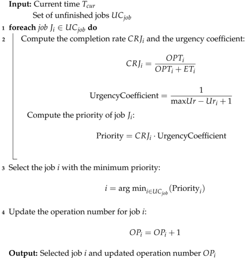 |
5.2.2. Scheduling Rule 2 for Sub-Task 1
For rule 2 of sub-task 1, begin by defining the set of unfinished jobs, . From this set, extract the delayed jobs , where the delivery deadline has been exceeded, to form a set of tardy jobs, . If delayed jobs exist, prioritize those with the longest overdue time and highest urgency. If no delayed jobs are present, select jobs from the set which exhibit a smaller difference between their overdue time and estimated completion time, combined with high urgency. The detailed procedure is outlined in Algorithm 2.
| Algorithm 2: Procedure for Dispatching Rule 2 in Sub-task 1 |
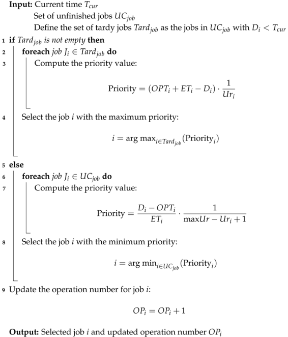 |
5.2.3. Scheduling Rule 3 for Sub-Task 1
The third dispatching rule for sub-task 1 involves randomly selecting a job and processing its next operation. The procedure is expressed in Algorithm 3.
| Algorithm 3: Procedure for Dispatching Rule 3 in Sub-task 1 |
|
Input: Current time Set of unfinished jobs
|
5.2.4. Scheduling Rule 1 for Sub-Task 2
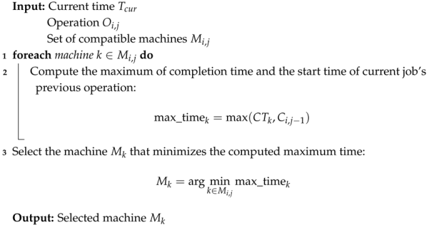
After selecting the operation to be processed, a set of available machines from its compatible machine set , which are neither broken down nor undergoing tool changes, can be identified. The goal of the second sub-task is to allocate the operation to a suitable machine . Rule 1 selects the machine that can provide service the earliest for operation , thereby enhancing the average machine utilization rate . The detailed procedure is illustrated in Algorithm 4.
| Algorithm 4: Procedure for Dispatching Rule 1 in Sub-task 2 |
 |
5.2.5. Scheduling Rule 2 for Sub-Task 2
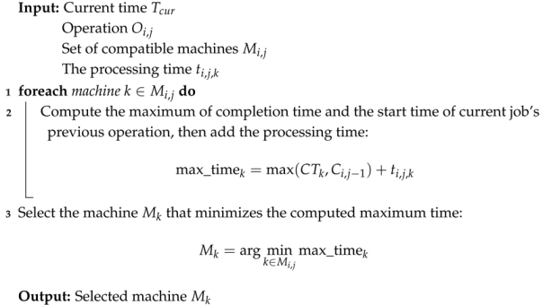
The second scheduling rule of sub-task 2 builds on the first rule by combining the processing time of operation on machine with the earliest available time. This rule takes both the availability time and processing capability into account. The process is outlined in Algorithm 5.
| Algorithm 5: Procedure for Dispatching Rule 2 in Sub-task 2 |
 |
5.2.6. Scheduling Rule 3 for Sub-Task 2
To enhance the robustness of the scheduling process and avoid local optima, a random selection rule is recommended as the third rule for sub-task 2. The step-by-step procedure can be found in Algorithm 6.
| Algorithm 6: Procedure for Dispatching Rule 3 in Sub-task 2 |
Input: Current time Operation Set of compatible machines Output: Selected machine |
By combining the rules of sub-task 1 and sub-task 2, nine composite scheduling rules are generated. This design enhances the flexibility and diversity of the scheduling strategies. The job sequencing and machine allocation rules address multiple scheduling needs, such as job delays, machine availability, and urgency, while also handling the impact of six dynamic events on the system. These combined rules form various scheduling strategies, allowing the system to adapt to complex production scenarios and improving its overall adaptability.
Although the rule set contains only nine composite rules, they effectively cover the main production scheduling needs. First, rules 1 and 2 prioritize jobs with higher delays and urgency, ensuring timely scheduling and proper prioritization. They address the conflict between job completion rate and deadlines, especially when dynamic events, such as job insertion or modification occur, enabling quick strategy adjustments. Second, rules 1 and 2 consider machine availability and job processing time to select the most suitable machines. This improves machine utilization () and reduces production bottlenecks, especially when dynamic events like machine breakdowns or tool changes affect the system, ensuring optimal resource allocation.
5.3. Definition of Reward Function
In the deep Q-learning algorithm, when different actions are executed in state , the agent transitions to a new state , and this process generates a corresponding reward . The magnitude of the reward directly influences the agent’s strategy selection, determining how it will choose the next action in subsequent states. To achieve multi-objective optimization, this study uses a Dual-Level Integrated Deep Q-Network structure and switches between different reward mechanisms. However, using makespan as the optimization goal leads to a sparse reward problem in reinforcement learning. In DMOFJSP, makespan is only determined once all operations for each job are completed. This means that the agent cannot obtain immediate feedback on makespan during the early stages of scheduling. The agent only receives a final reward based on the maximum completion time when all jobs are finished. Before that, there is little reward signal related to makespan optimization, making it difficult to learn effective strategies. To address this, the study uses job tardiness rate () and machine utilization rate () as the main reward mechanisms. These two objectives provide timely feedback after each decision, helping the agent make better choices faster and improving the scheduling strategy, which indirectly helps reduce makespan.
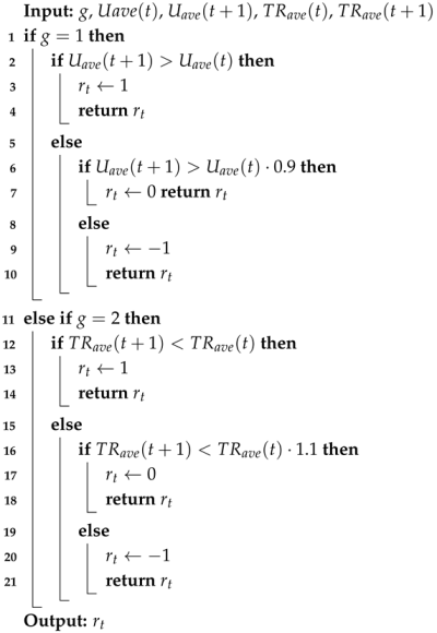
Specifically, the high-level IDQN first receives the state features as input, and based on this input, it outputs different goal values . When the high-level IDQN selects a goal value g, the low-level IDQN chooses distinct reward algorithms depending on the selected goal. If , the reward algorithm is based on the average machine utilization rate , as defined in Equations (13) and (16). If , the reward algorithm focuses on the average job processing tardiness rate , defined in Equations (14) and (20). The detailed execution process of these two distinct reward algorithms is outlined in the pseudocode in Algorithm 7.
| Algorithm 7: Reward Calculation Based on or |
 |
This multi-objective optimization approach enables the agent to flexibly choose different reward mechanisms, allowing it to balance machine utilization and job tardiness rates in complex dispatching tasks, ultimately optimizing overall scheduling performance.
5.4. Local Search Algorithm
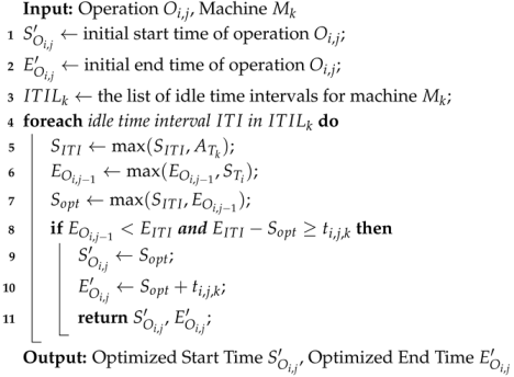
This study uses a unique local search algorithm to determine the processing time interval for operation on machine . The algorithm focuses on selecting idle time intervals for local optimization, which is essential for solving the DMOFJSP. This problem involves dynamic events, such as job insertions and machine breakdowns, making the scheduling process complex and uncertain. Idle time intervals, which represent machine downtime, provide a flexible optimization space. By scheduling jobs within these intervals, machine utilization is maximized, resource wastage is avoided, and scheduling conflicts caused by unexpected events are reduced. The local optimization targets the best idle time intervals, ensuring proper job sequencing and resource allocation. This reduces computational load and speeds up the optimization process. Overall, this method enhances the system’s adaptability and stability in dynamic environments, effectively addressing varying scheduling needs while optimizing objectives like minimizing makespan, maximizing , and minimizing .
The search process is detailed in Algorithm 8. We create an idle time interval list for machine , consisting of idle time intervals, denoted as . Next, we search through the list for idle time intervals that satisfy the following conditions: we search for intervals where the end time is later than the end time of operation , and the duration is long enough to accommodate the processing time of . Once a suitable idle time interval is found, we schedule operation within that interval. During scheduling, we ensure that the start time of the idle time interval is no earlier than the availability time of machine , and the end time of the previous operation is later than the start time of the job. These time constraints are crucial for ensuring the feasibility and effectiveness of the scheduling plan.
| Algorithm 8: Local Search Process |
 |
5.5. The Network of the DLIDQN
The proposed DLIDQN framework integrates multiple network structures, consisting of two IDQNs. Each IDQN is primarily composed of a dueling DQN model and includes noisy layers to enhance exploration capabilities. The higher-level IDQN model consists of three hidden layers, each with ten nodes. It takes a 6-dimensional state feature as input and outputs a Q-value that combines the state value and advantage function, where the state value branch outputs one node, and the advantage function branch outputs two nodes, corresponding to the two high-level optimization goals (i.e., the two forms of reward functions). The lower-level IDQN model is more complex, containing seven hidden layers, each with 50 nodes. With a 7-dimensional state feature (six state features and one high-level goal) as input, it calculates the final Q-value by combining the state value and the advantage function. The advantage function branch produces nine nodes, each corresponding to one of the nine composite scheduling rules. Both models use the ReLU activation function and are optimized with the mean square error (MSE) loss function and the Adam optimizer. At each rescheduling event, scheduling rules are executed to generate a new state, and a reward algorithm is selected based on the goal values to obtain corresponding rewards. The state, action, reward, new state, reward function targets, and completion indicator are stored for prioritized experience replay to update the network parameters. Figure 1 illustrates the structure of the proposed DLIDQN and the overall algorithm process.
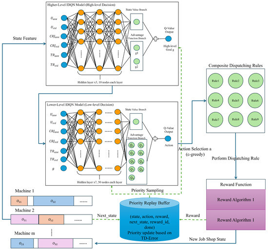
Figure 1.
The structure of DLIDQN and the overall algorithm process.
6. Numerical Experiments
A detailed account of the numerical experiments used to assess the effectiveness and generalization of the DLIDQN framework is provided in this section, along with an analysis of the results. We first introduce the parameter settings of the dataset and algorithms used during the training and testing process. After completing the training, we evaluate the DLIDQN model against each composite dispatching rule introduced in this study, as well as commonly adopted classic dispatching rules. To further highlight the strengths of the proposed model, we compare DLIDQN with three other deep reinforcement learning algorithms that utilize the same action space of nine composite dispatching rules. Through experiments and visualizations, the high performance and strong generalization capability of the DLIDQN model are confirmed.
6.1. Training Process
This section explains the model training process, which is carried out over 200 runs using randomly generated data. To ensure the model can adapt to different workshop configurations, the initial number of jobs, machines, operations per job, and new job insertions are varied randomly during each training session. New jobs arrive according to a Poisson distribution, with the time between consecutive job insertions following an exponential distribution . Other environmental parameters are also randomly updated within a specified range. The instance parameters used during training are listed in Table 3. The number of machines available for each operation is randomly generated, with a maximum of to ensure at least two machines are always available.
Table 3.
Parameter settings for various production configurations in the training process.
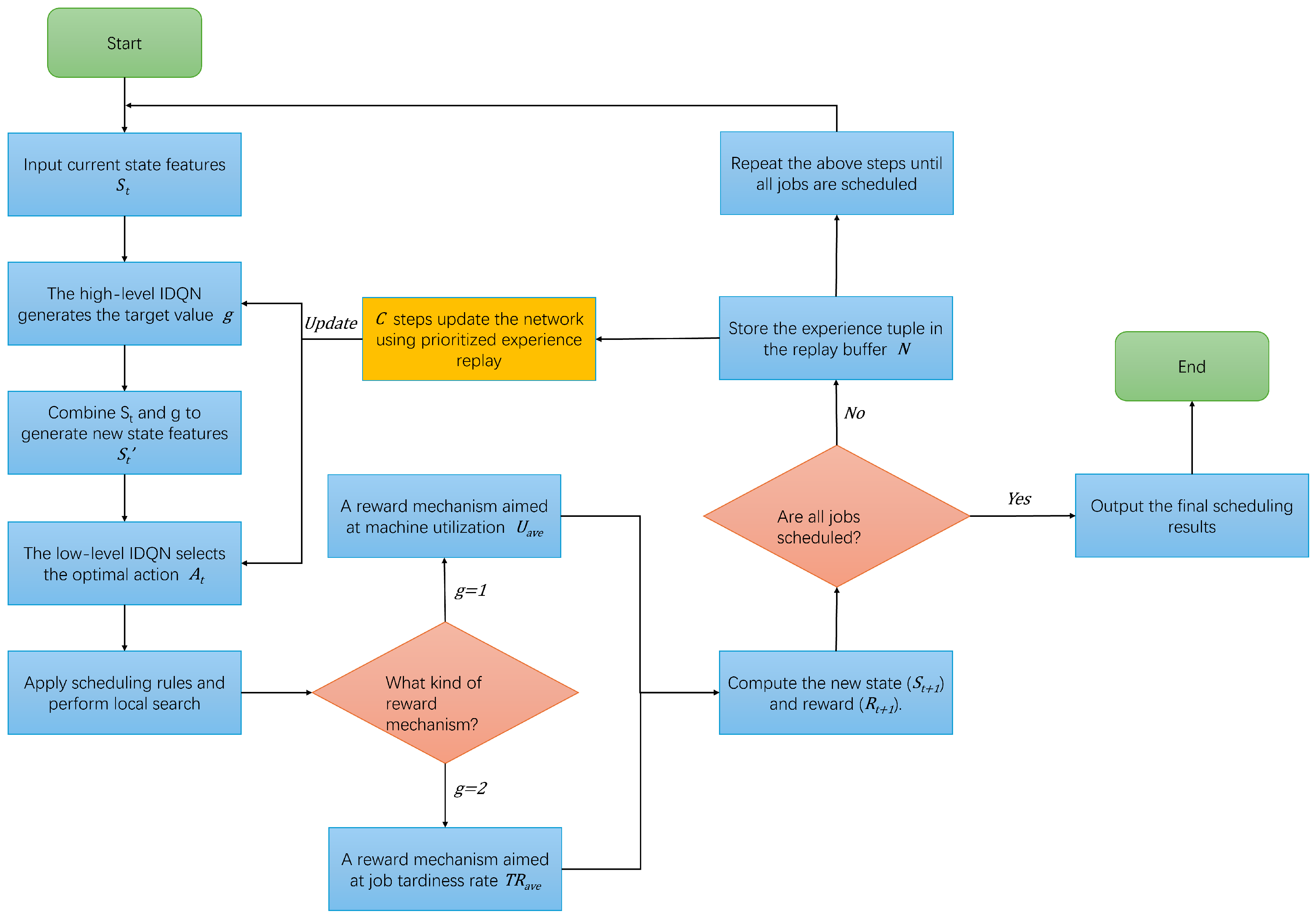
Figure 2 illustrates the training logic flow of the DLIDQN model. During the training process, the dual IDQN models collaborate to optimize performance. First, the high-level model receives the state feature and generates the target value g, then combines and g to create a new state , which is passed to the low-level model. The low-level model selects action based on , applies the scheduling rules, and uses a local search algorithm to improve the results. Next, the new state is calculated, and the reward is obtained. If all jobs are scheduled, the final results are output, marking the end of the training. Otherwise, the tuple is saved in the replay buffer. After the defined step count is reached, the prioritized experience replay mechanism is used to update the network parameters, continuing the process until all jobs are scheduled.
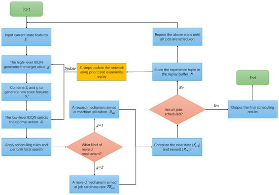
Figure 2.
Dynamic multi-objective scheduling workflow of DLIDQN.
Table 4 lists the parameter settings for the training algorithm. Most of these parameters are based on pre-experimental results, while some use common default values from deep reinforcement learning algorithms. Specifically, the buffer capacity is set to 2000. When the capacity is exceeded, old data will be overwritten to make space for new data. The learning rate () is set to 0.001, balancing convergence speed and model stability. Pre-experimental results show that a high learning rate can cause instability, while a low learning rate slows convergence, making it hard to achieve good results in a limited number of iterations. The target network update frequency (C) is set to 200 steps. Regular updates help stabilize the training process and reduce fluctuations. The experiments also found that too low of an update frequency causes significant fluctuations, while too high of a frequency can slow down convergence.
Table 4.
Hyperparameter settings for the training algorithm.
A test instance containing 16 machines, with set to 70 and 40 new job insertions, was prepared to validate the DLIDQN model obtained after each training round. During testing, the curve of makespan for each training round and the average makespan over every 20 training rounds are shown in Figure 3. The graph shows the trend of average makespan achieved by DLIDQN during each training epoch. The green “Makespan” curve represents the makespan for each epoch, with some fluctuations. The red “Average Makespan Obtained Every 20 Training Epochs” line demonstrates a steady decline as training progresses.
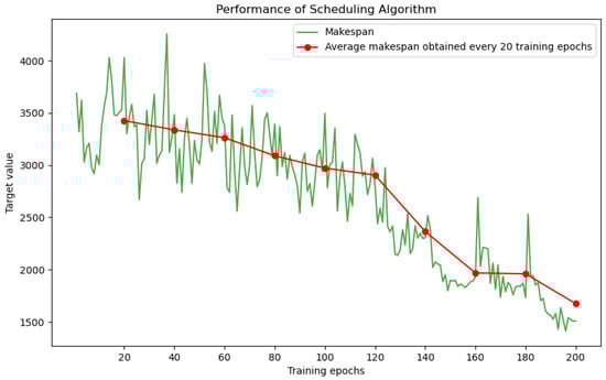
Figure 3.
Average makespan achieved by DLIDQN at each training epoch. The green “Makespan” curve represents the makespan recorded for each epoch. The red “Average makespan obtained every 20 training epochs” line indicates the average makespan over every 20 epochs.
In the first 100 epochs, the makespan decreases quickly, indicating that the model is learning the key features of the task. Between 100 and 200 epochs, the decline slows, suggesting that the model is entering a fine-tuning phase. After 200 epochs, the makespan stabilizes, and further training does not significantly improve performance.
Comparing the performance across different epochs shows that there is still room for improvement after 100 epochs. However, after 200 epochs, the makespan reaches its lowest point. The small performance gap between 150 and 200 epochs indicates that 200 epochs are enough to cover the task’s complexity and achieve effective learning. Moreover, the use of diverse training instances ensures the model’s ability to generalize and perform well in different production environments. Therefore, 200 training epochs are sufficient for the model to reach optimal training and provide strong scheduling performance.
6.2. Testing Settings
After completing model training, the evaluation phase begins, with all test samples generated randomly. Table 5 shows the specific parameters for each test sample. The initial number of jobs is set to 20, 30, or 40, with the number of operations per job assigned arbitrarily and processing times for each operation determined randomly. The number of machines is initialized to 8, 12, or 16 units, and the number of dynamic events is selected randomly from 30, 50, or 70, with event types also allocated at random. Other parameters related to jobs and machines follow the same setup as in the training stage. A total of 27 distinct test configurations were established, each tested 20 times independently. These test configurations cover different task scales, machine numbers, and dynamic event distributions, validating the robustness of the DLIDQN model in complex dynamic environments. The results show that despite significant randomness and uncertainty in the input parameters, the model consistently produces high-quality scheduling results. This demonstrates that the DLIDQN model can adapt to changes in task scale, processing time fluctuations, and disruptions from dynamic events. This robustness highlights the model’s wide applicability and reliability in real-world production environments.
Table 5.
Parameter settings for various production configurations in the testing process.
The testing was implemented in Python, running in a Python 3.8 environment on a computer with an Intel i7-9750H processor, 24 GB of RAM, and a GTX 1650Ti graphics card. In this setup, we compared the performance of our DLIDQN algorithm against the baseline algorithms using the same set of test cases.
6.3. Comparisons with the Proposed Composite Dispatching Rules
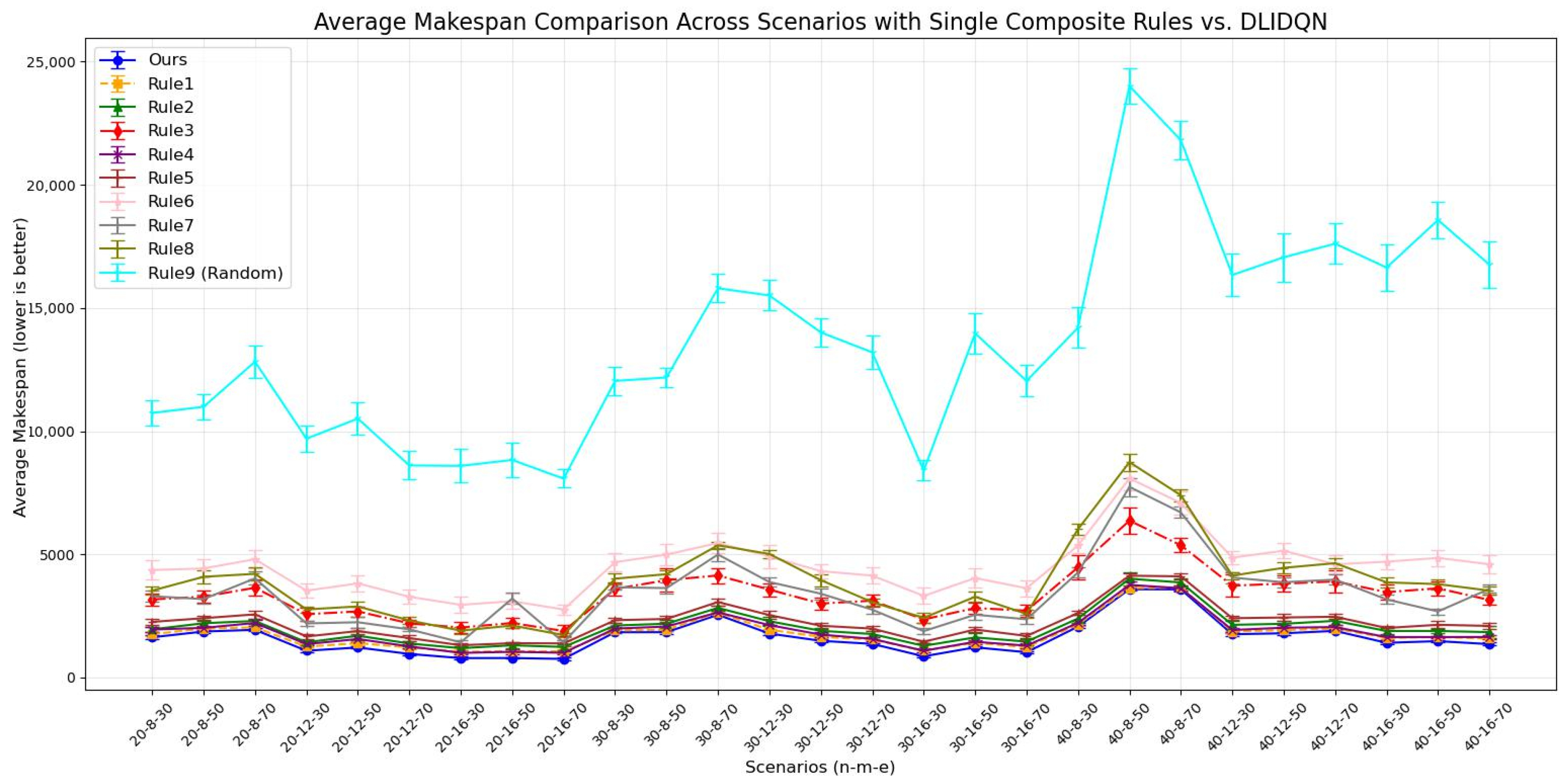
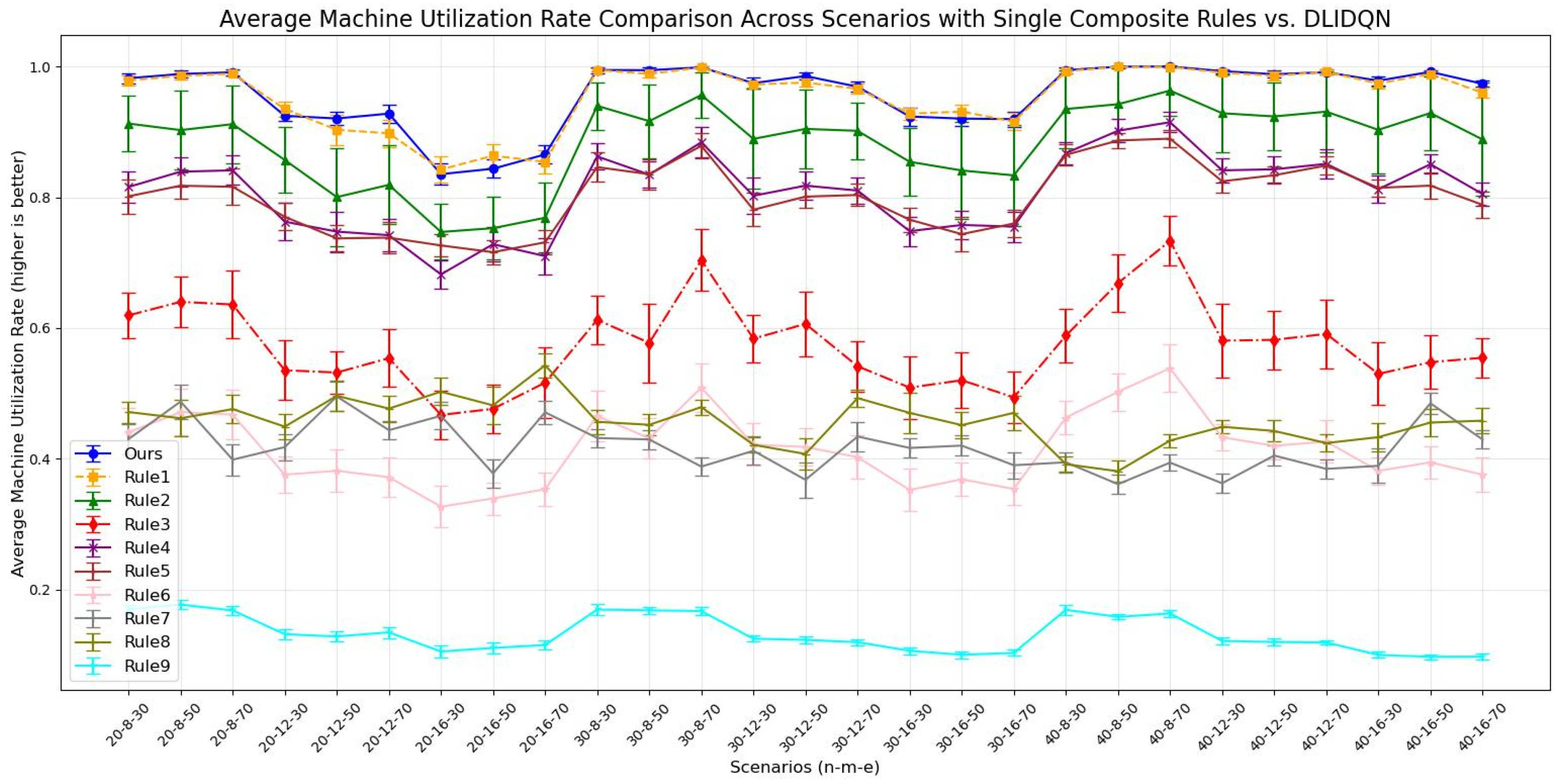
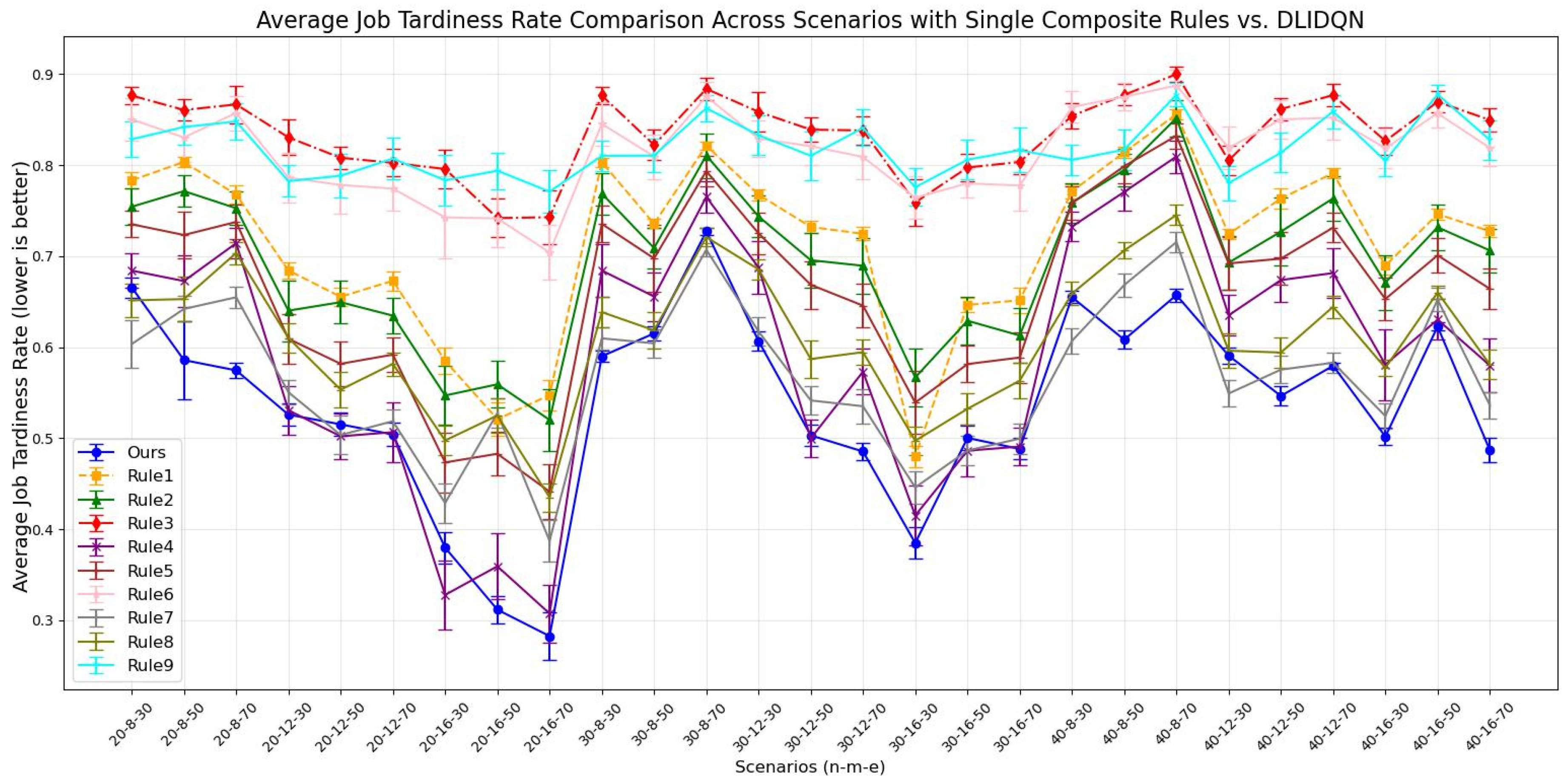
To assess the performance of DLIDQN, this study conducted 20 independent experiments on each of 27 test instances with various parameter configurations, comparing DLIDQN with the proposed nine composite scheduling rules. During the experiments, we calculated the mean and standard deviation of makespan, , and across 20 runs for each instance and summarized the results in Table 6, Table 7 and Table 8, where the best performance values are highlighted in bold. To more intuitively present the data in the tables, we created corresponding line charts (Figure 4, Figure 5 and Figure 6) to compare the performance of single composite rules and DLIDQN across different scenarios. These line charts clearly illustrate DLIDQN’s advantages in key metrics such as average makespan, average utilization, and average turnaround time, further demonstrating its superior performance under various parameter configurations.
Table 6.
Analysis of the averages and standard deviations of makespan across 20 runs for single composite rules vs. DLIDQN.
Table 7.
Analysis of the averages and standard deviations of across 20 runs for single composite rules vs. DLIDQN.
Table 8.
Analysis of the averages and standard deviations of across 20 runs for single composite rules vs. DLIDQN.

Figure 4.
Average makespan comparison across scenarios with single composite rules vs. DLIDQN.
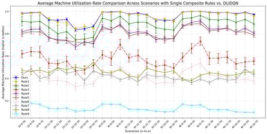
Figure 5.
Average machine utilization rate comparison across scenarios with single composite rules vs. DLIDQN.
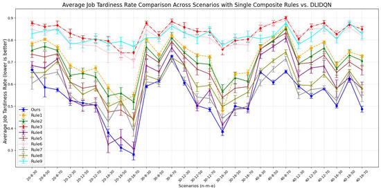
Figure 6.
Average job tardiness rate comparison across scenarios with single composite rules vs. DLIDQN.
The results show that DLIDQN, with its action space covering nine scheduling rules, can flexibly select the best rules for composite scheduling. This allows it to outperform most single scheduling rules in various production environments. In comparisons with the random strategy (Rule 9), DLIDQN performs better in nearly all test cases. However, in some scenarios, its performance is slightly lower than certain single rules. For example, in the metric, DLIDQN falls short of Rule 1 in six instances. Rule 1 prioritizes urgent jobs by calculating their completion rate and urgency coefficient. It also selects machines that can start jobs earlier, minimizing idle time. Similarly, DLIDQN’s is slightly worse than Rules 4 and 7 in some cases, as these rules also prioritize urgent jobs. Single scheduling rules are simple and clear, requiring fewer calculations. This makes them faster and more efficient in certain test cases, avoiding the complexity and computational costs of DLIDQN while achieving better performance in specific scenarios.
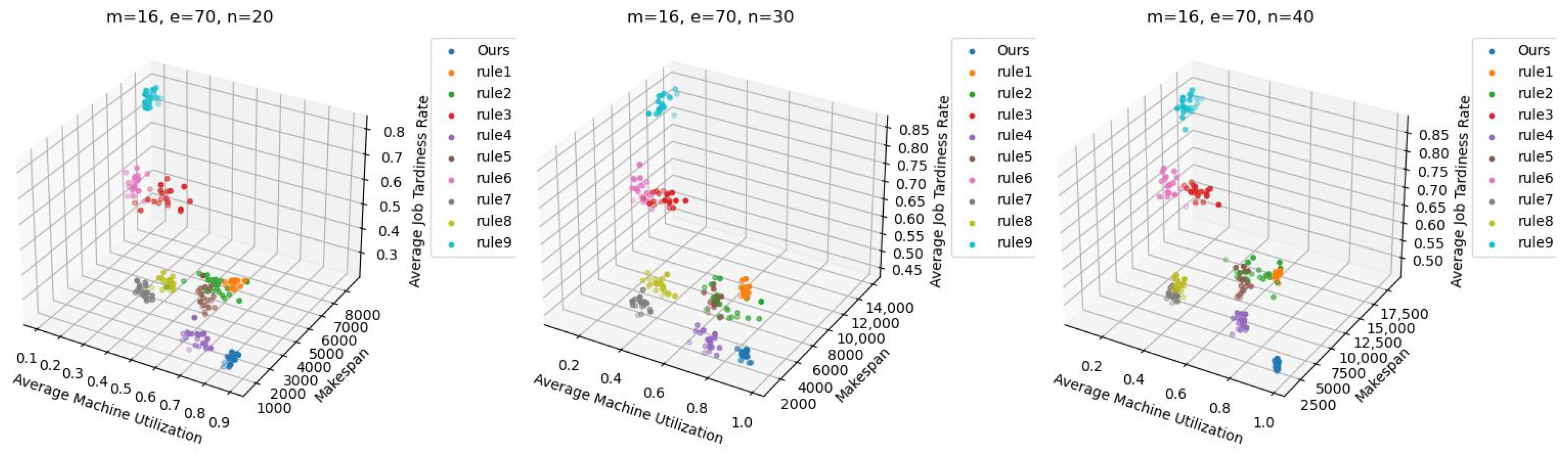
DLIDQN may require more computation and strategy exploration during learning, which can lead to suboptimal performance in some cases. However, no single scheduling rule can consistently achieve optimal results across various production environments. This demonstrates DLIDQN’s strong adaptability and excellent performance when handling untrained production configurations. Figure 7 shows the three-dimensional Pareto front for DLIDQN and composite scheduling rules in three test cases, further proving the superiority of the DLIDQN model.
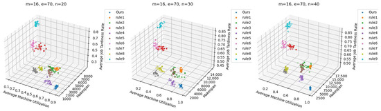
Figure 7.
Pareto fronts obtained by DLIDQN and the proposed composite dispatching rules after 20 runs on three representative instances.
6.4. Comparisons with Classic Dispatching Rules
We compared DLIDQN with five widely recognized classic dispatching rules to more comprehensively validate its superiority, followed by a detailed explanation of each rule.
- First In First Out (FIFO): Decide the next operation to start based on the arrival time of jobs, selecting the next operation for the job that arrived first.
- Earliest Due Date (EDD): Sort jobs by their due dates and choose the next operation for the job with the earliest due date to ensure timely delivery.
- Shortest Processing Time (SPT): Schedule based on the estimated shortest time required to complete each job, selecting the next operation for the job with the shortest processing time.
- Longest Processing Time (LPT): Opposite to SPT, choose the job with the longest processing time, typically used for optimizing resource allocation to expedite the processing of tasks that have been waiting longer.
- Most Remaining Processing Time (MRT): Consider jobs with the most remaining processing time (those with the longest remaining time) to balance the overall schedule.
It should be noted that the aforementioned classic scheduling strategies lack explicit machine assignments when handling job allocations, making them difficult to adapt to the flexible job shop scheduling problem (FJSP) addressed in this paper. To overcome this shortcoming, we established a supplementary machine assignment principle: for each job, we select the earliest available machine from its compatible set for job allocation, allowing for a fair performance comparison between these classic strategies and our method.
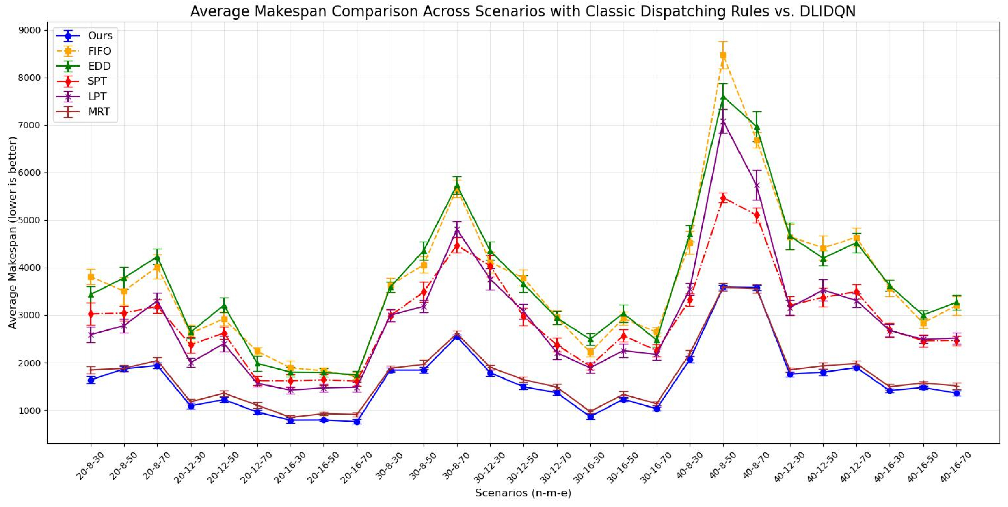
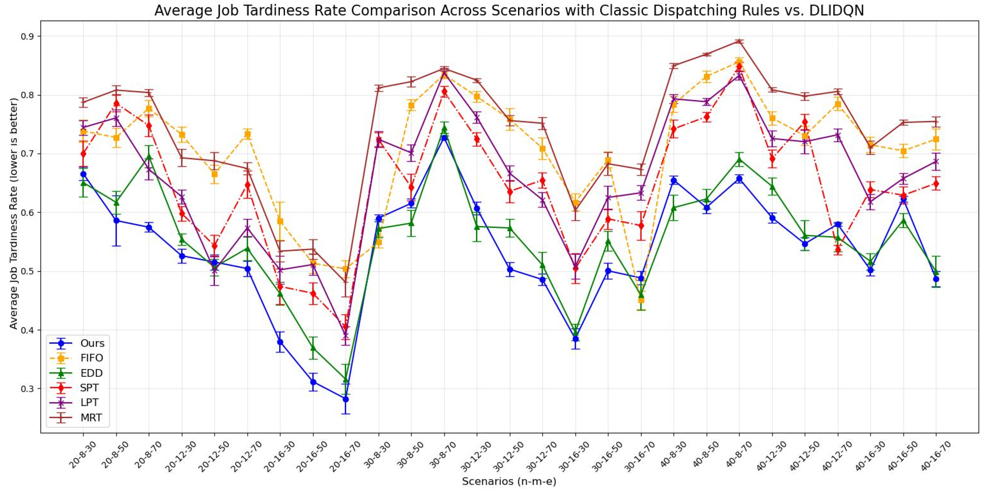
We independently conducted 20 experiments for each test instance, and the results are summarized in Table 9, Table 10 and Table 11. These tables provide the averages and standard deviations for three key performance indicators: makespan, average machine utilization (), and average tardiness rate (). The optimal values are highlighted in bold. The line charts corresponding to the tables are shown in Figure 8, Figure 9 and Figure 10. After analyzing the data, we found that our algorithm performs better than traditional scheduling strategies in most test cases across all three performance metrics. Although in some scenarios, the DLIDQN framework performs slightly worse than EDD in terms of , this is because EDD prioritizes jobs with the earliest due dates, effectively reducing tardiness risk. In cases where due dates are closely distributed or many jobs are urgent, EDD’s focus on due dates helps lower the average tardiness rate. In comparison, the framework uses dynamic rule selection to optimize multiple objectives, so it does not always prioritize the most urgent jobs. However, it achieves the best performance in most instances. In certain specific cases, the difference in between the framework and the optimal value is small. Therefore, the experimental results show that the proposed composite scheduling rules are effective in reducing tardiness and improving machine utilization.
Table 9.
Analysis of the averages and standard deviations of makespan across 20 runs for classic dispatching rules vs. DLIDQN.
Table 10.
Analysis of the averages and standard deviations of across 20 runs for classic dispatching rules vs. DLIDQN.
Table 11.
Analysis of the averages and standard deviations of across 20 runs for classic dispatching rules vs. DLIDQN.

Figure 8.
Average makespan comparison across scenarios with classic dispatching rules vs. DLIDQN.
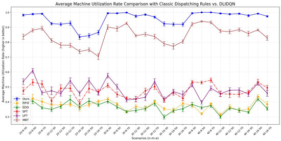
Figure 9.
Average machine utilization rate comparison with classic dispatching rules vs. DLIDQN.
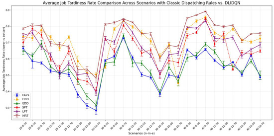
Figure 10.
Average job tardiness rate comparison across scenarios with classic dispatching rules vs. DLIDQN.
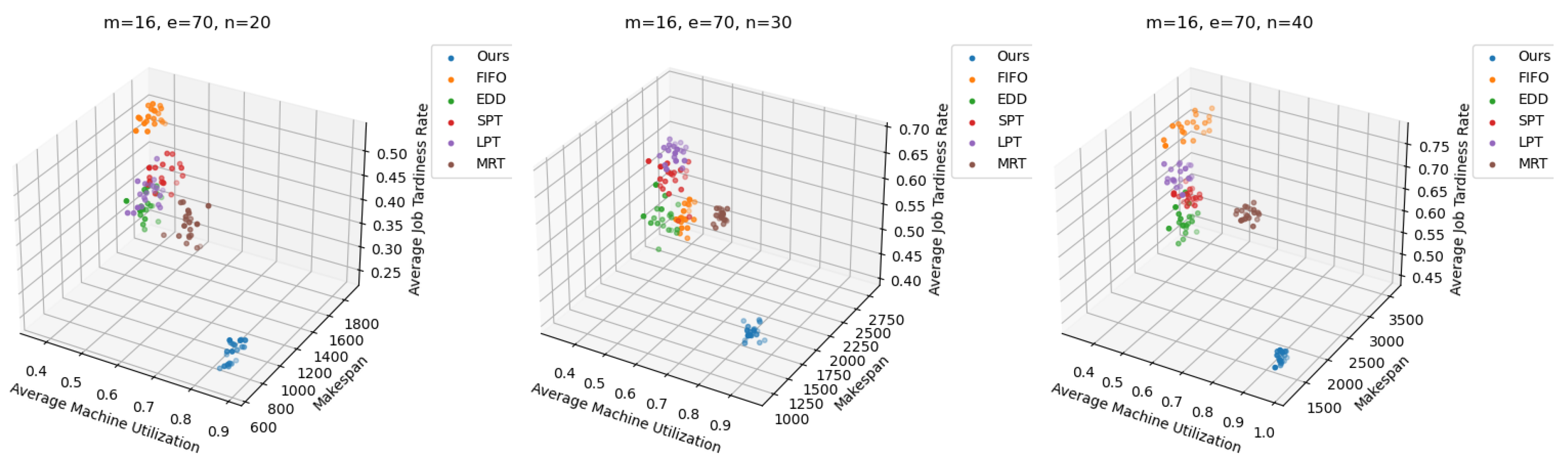
Furthermore, as shown in Figure 11, the Pareto optimal front clearly highlights DLIDQN’s advantage over other well-known dispatching rules in a range of representative instances.

Figure 11.
Pareto fronts obtained by DLIDQN and well-known classic dispatching rules after 20 runs on three representative instances.
6.5. Comparisons with Other RL-Based Scheduling Algorithms
In order to demonstrate the superiority of our method for multi-objective optimization tasks, we carried out a comprehensive comparison, evaluating DLIDQN against three mainstream reinforcement learning-based training algorithms. These three algorithms are DQN (the classic Deep Q-Network), dueling double DQN (D3QN, an improved architecture of double DQN), and HDMDDQN, a novel two-layer deep double Q-network training method proposed by Wang et al. (2022) [43].
DQN, as the control group, features a simple design, relying on a single RL agent for rule selection without higher-level scheduling objectives. Details of its reward mechanism are provided in Algorithm 9. For fairness, all methods share the same action space as DLIDQN, consisting of nine composite scheduling rules. We compared the means and standard deviations of makespan, , and across various production environments. The results are presented in Table 12, Table 13 and Table 14. The optimal values are highlighted in bold. The line charts corresponding to the tables are shown in Figure 12, Figure 13 and Figure 14.
| Algorithm 9: DQN Reward Algorithm |
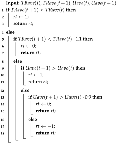 |
Table 12.
Analysis of the averages and standard deviations of makespan across 20 runs for other RL-based algorithms vs. DLIDQN.
Table 13.
Analysis of the averages and standard deviations of across 20 runs for other RL-based algorithms vs. DLIDQN.
Table 14.
Analysis of the averages and standard deviations of across 20 runs for other RL-based algorithms vs. DLIDQN.
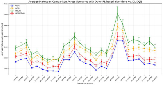
Figure 12.
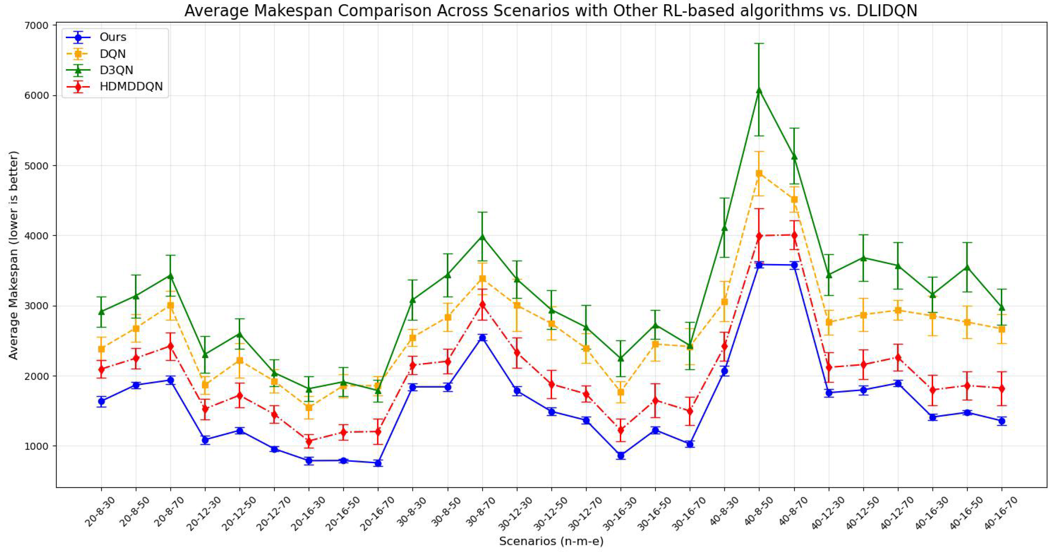
Average makespan comparison across scenarios with other RL-based algorithms vs. DLIDQN.
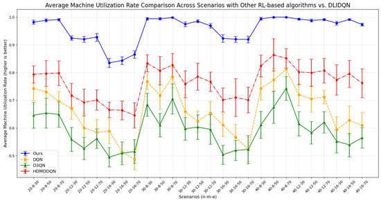
Figure 13.
Average machine utilization rate comparison across scenarios with other RL-based algorithms vs. DLIDQN.
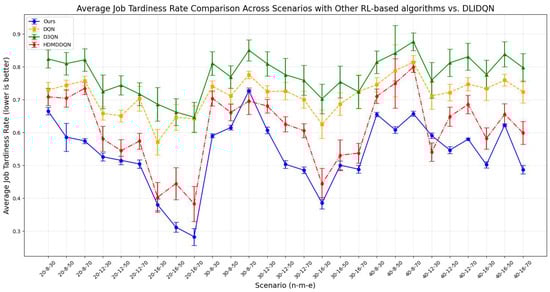
Figure 14.
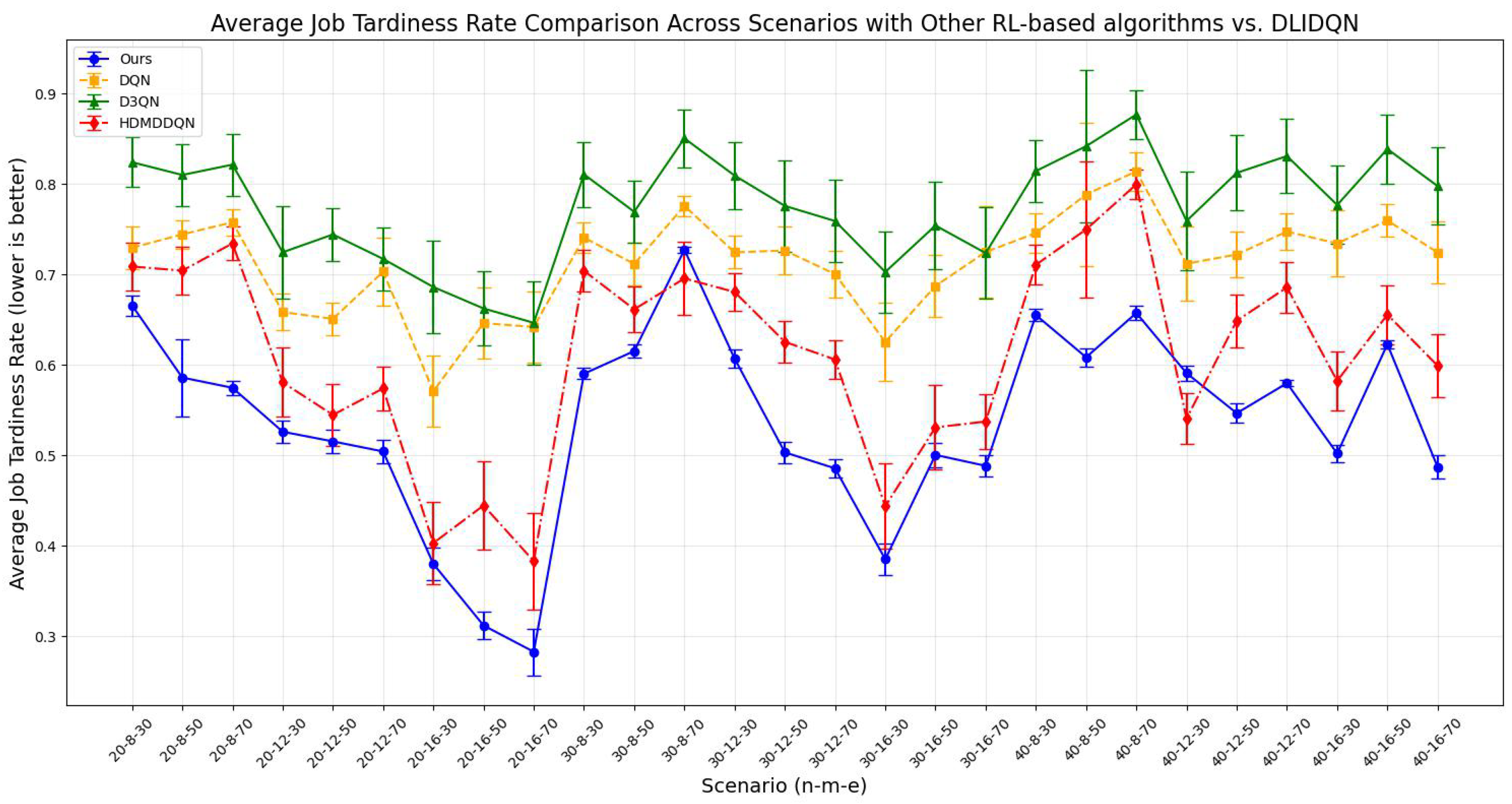
Average job tardiness rate comparison across scenarios with other RL-based algorithms vs. DLIDQN.
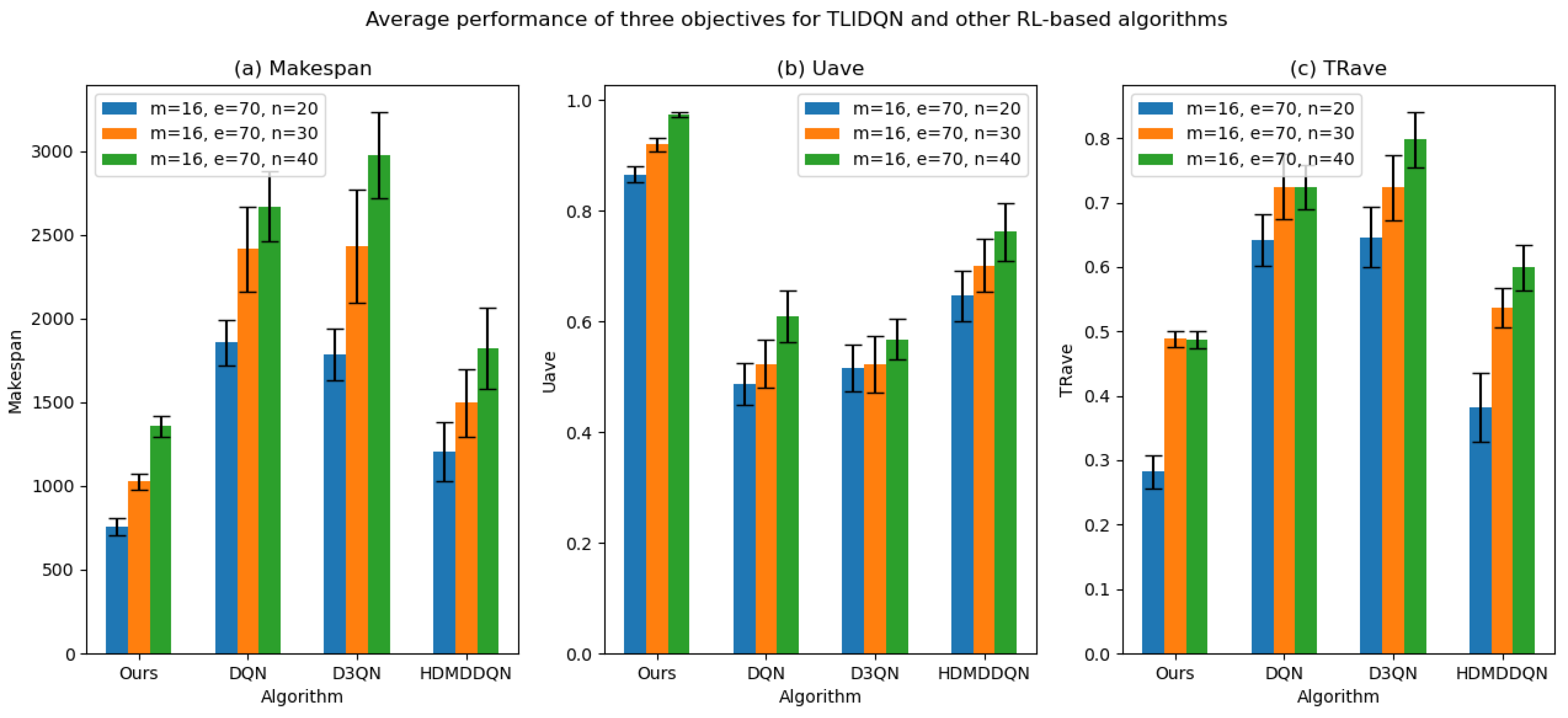
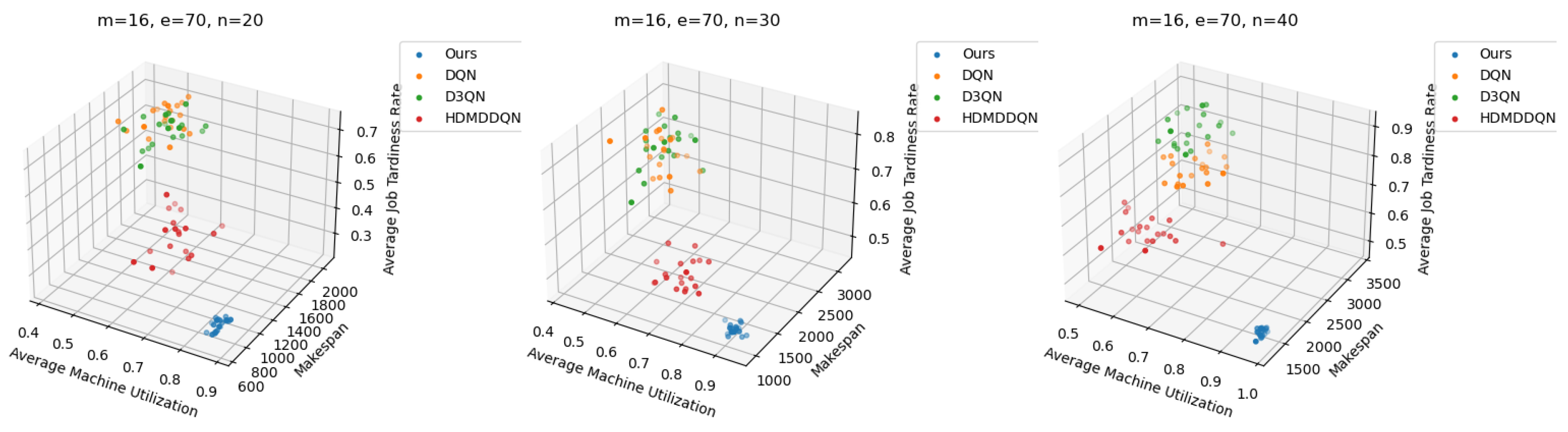
The comparison results show that DLIDQN demonstrates a significant advantage over other RL training methods in the vast majority of test instances. Through performance comparisons with the single-layer DQN, we convincingly prove that the proposed two-layer structure is not only indispensable but also exhibits high effectiveness in practical applications. The high-level DQN component of DLIDQN intelligently selects the optimal optimization objective at different rescheduling points, thereby achieving an excellent balance among makespan, , and . Additionally, compared to the other two advanced algorithms with a dual-layer structure, our proposed DLIDQN model, which integrates multiple network structures and a prioritized experience replay mechanism, also displays significant performance advantages, further highlighting the exceptional capabilities of DLIDQN. In Figure 15, the performance of DLIDQN and various RL-based methods is evaluated across multiple representative instances for three objectives. It is clear that DLIDQN outperforms the others in all three objectives. Moreover, a view of Figure 16 indicates that our method remains at the forefront of the Pareto optimal front. The results from the Pareto chart and other graphs show that DLIDQN performs well in reducing completion time, improving resource utilization, and lowering delay rates. This proves its advantage in single-objective optimization and also demonstrates its strong performance in multi-objective optimization, highlighting its efficiency and broad applicability in practical scenarios.
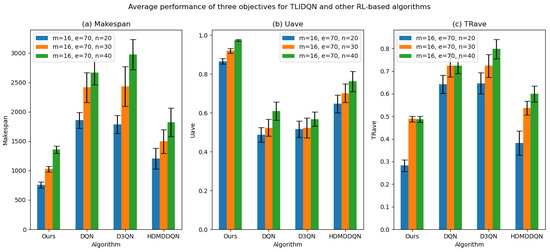
Figure 15.
The average performance of DLIDQN and other RL-based algorithms across three objectives was calculated for three representative instances.
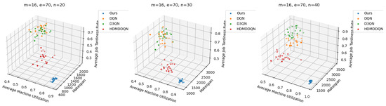
Figure 16.
Pareto fronts obtained by DLIDQN and other RL-based algorithms after 20 runs on three representative instances.
7. Conclusions
This paper presents the Dual-Level Integrated Deep Q-Network (DLIDQN) algorithm, which provides an effective solution to the dynamic multi-objective flexible job shop scheduling problem (DMOFJSP), involving six dynamic events: new job insertions, job cancellation, job operation modification, machine addition, machine tool replacement and machine breakdown. The algorithm implements goal-oriented scheduling through dual IDQN agents. At rescheduling moments, the high-level IDQN dynamically generates an optimization target for the low-level IDQN based on the current state features. The low-level IDQN, guided by this goal and considering the state features, executes the most suitable scheduling rules to ensure the achievement of the specified goals. In addition, DLIDQN integrates the benefits of diverse network architectures, resulting in powerful optimization capabilities. By designing two reward algorithms and six essential state features, as well as developing nine composite scheduling rules, the algorithm demonstrates outstanding performance in optimizing makespan, average machine utilization (), and average job processing tardiness rate ().
To comprehensively assess the performance and generalization ability of DLIDQN, a series of extensive numerical experiments were conducted across various shop configurations. The results indicate that DLIDQN not only outperforms all the proposed composite scheduling rules but also surpasses existing classical scheduling rules and other reinforcement learning-based scheduling methods. Notably, DLIDQN performs exceptionally well in untrained production environments, demonstrating its remarkable algorithmic performance and adaptability.
Future research will focus on exploring the application of advanced policy-based algorithms, such as actor–critic (AC) and Proximal Policy Optimization (PPO), to dynamic multi-objective flexible job shop scheduling problems (DMOFJSP). Additionally, we plan to investigate multi-agent reinforcement learning (MARL) to analyze how multiple agents can achieve their goals through interactive learning in a shared environment. By integrating these insights with policy-based training methods, we aim to further enhance the performance of scheduling algorithms in complex dynamic environments.
Author Contributions
Conceptualization, H.X., J.Z., L.H. and J.T.; methodology, H.X., J.Z. and C.Z.; software, H.X., J.Z. and J.T.; validation, H.X., J.Z. and L.H.; formal analysis, J.Z. and C.Z.; writing—original draft preparation, H.X. and J.Z.; writing—review and editing, L.H., J.T. and C.Z.; visualization, H.X. and J.Z.; supervision, L.H., J.T. and C.Z.; project administration, H.X. All authors have read and agreed to the published version of the manuscript.
Funding
This research received no external funding.
Data Availability Statement
No new data were created or analyzed in this study.
Conflicts of Interest
The authors declare no conflicts of interest.
References
- Garey, M.R.; Johnson, D.S.; Sethi, R. The Complexity of Flowshop and Jobshop Scheduling. Math. Oper. Res. 1976, 1, 117–129. [Google Scholar] [CrossRef]
- Ouelhadj, D.; Petrovic, S. A survey of dynamic scheduling in manufacturing systems. J. Sched. 2009, 12, 417–431. [Google Scholar] [CrossRef]
- Lou, P.; Liu, Q.; Zhou, Z.; Wang, H.; Sun, S.X. Multi-agent-based proactive–reactive scheduling for a job shop. Int. J. Adv. Manuf. Technol. 2012, 59, 311–324. [Google Scholar] [CrossRef]
- Pezzella, F.; Morganti, G.; Ciaschetti, G. A genetic algorithm for the Flexible Job-shop Scheduling Problem. Comput. Oper. Res. 2008, 35, 3202–3212. [Google Scholar] [CrossRef]
- Kundakcı, N.; Kulak, O. Hybrid genetic algorithms for minimizing makespan in dynamic job shop scheduling problem. Comput. Ind. Eng. 2016, 96, 31–51. [Google Scholar] [CrossRef]
- Ning, T.; Huang, M.; Liang, X.; Jin, H. A novel dynamic scheduling strategy for solving flexible job-shop problems. J. Ambient Intell. Humaniz. Comput. 2016, 7, 721–729. [Google Scholar] [CrossRef]
- Cruz-Chávez, M.A.; Martínez-Rangel, M.G.; Cruz-Rosales, M.H. Accelerated simulated annealing algorithm applied to the flexible job shop scheduling problem. Int. Trans. Oper. Res. 2017, 24, 1119–1137. [Google Scholar] [CrossRef]
- Zhu, Z.; Zhou, X. An efficient evolutionary grey wolf optimizer for multi-objective flexible job shop scheduling problem with hierarchical job precedence constraints. Comput. Ind. Eng. 2020, 140, 106280. [Google Scholar] [CrossRef]
- El Khoukhi, F.; Boukachour, J.; Alaoui, A.E.H. The “Dual-Ants Colony”: A novel hybrid approach for the flexible job shop scheduling problem with preventive maintenance. Comput. Ind. Eng. 2017, 106, 236–255. [Google Scholar] [CrossRef]
- Zhang, S.; Li, X.; Zhang, B.; Wang, S. Multi-objective optimisation in flexible assembly job shop scheduling using a distributed ant colony system. Eur. J. Oper. Res. 2020, 283, 441–460. [Google Scholar] [CrossRef]
- Poppenborg, J.; Knust, S.; Hertzberg, J. Online scheduling of flexible job-shops with blocking and transportation. Eur. Ind. Eng. 2012, 6, 497–518. [Google Scholar] [CrossRef]
- Mohan, J.; Lanka, K.; Rao, A.N. A Review of Dynamic Job Shop Scheduling Techniques. Procedia Manuf. 2019, 30, 34–39. [Google Scholar] [CrossRef]
- Baker, K.R. Sequencing Rules and Due-Date Assignments in a Job Shop. Manag. Sci. 1984, 30, 1093–1104. [Google Scholar] [CrossRef]
- Nie, L.; Gao, L.; Li, P.; Li, X. A GEP-based reactive scheduling policies constructing approach for dynamic flexible job shop scheduling problem with job release dates. J. Intell. Manuf. 2013, 24, 763–774. [Google Scholar] [CrossRef]
- Sutton, R.S.; Barto, A.G. Reinforcement Learning: An Introduction; MIT Press: Cambridge, MA, USA, 2018. [Google Scholar]
- Aydin, M.; Öztemel, E. Dynamic job-shop scheduling using reinforcement learning agents. Robot. Auton. Syst. 2000, 33, 169–178. [Google Scholar] [CrossRef]
- Bouazza, W.; Sallez, Y.; Beldjilali, B. A distributed approach solving partially flexible job-shop scheduling problem with a Q-learning effect. IFAC-PapersOnLine 2017, 50, 15890–15895. [Google Scholar] [CrossRef]
- Wei, Y.; Zhao, M. Composite rules selection using reinforcement learning for dynamic job-shop scheduling. In Proceedings of the IEEE Conference on Robotics, Automation and Mechatronics, Singapore, 1–3 December 2004; Volume 2, pp. 1083–1088. [Google Scholar]
- Wang, Y.C.; Usher, J.M. Learning policies for single machine job dispatching. Robot. Comput.-Integr. Manuf. 2004, 20, 553–562. [Google Scholar] [CrossRef]
- Chen, R.; Yang, B.; Li, S.; Wang, S. A self-learning genetic algorithm based on reinforcement learning for flexible job-shop scheduling problem. Comput. Ind. Eng. 2020, 149, 106778. [Google Scholar] [CrossRef]
- Li, Y. Deep Reinforcement Learning: An Overview. arXiv 2017, arXiv:1701.07274. [Google Scholar]
- Wang, L.; Pan, Z.; Wang, J. A Review of Reinforcement Learning Based Intelligent Optimization for Manufacturing Scheduling. Complex Syst. Model. Simul. 2021, 1, 257–270. [Google Scholar] [CrossRef]
- Rafati, J.; Noelle, D.C. Learning representations in model-free hierarchical reinforcement learning. In Proceedings of the AAAI Conference on Artificial Intelligence, Honolulu, HI, USA, 27 January–1 February 2019; Volume 33, pp. 10009–10010. [Google Scholar]
- Li, A.C.; Florensa, C.; Clavera, I.; Abbeel, P. Sub-policy adaptation for hierarchical reinforcement learning. arXiv 2019, arXiv:1906.05862. [Google Scholar]
- Wei, Y.; Zhao, M. A reinforcement learning-based approach to dynamic job-shop scheduling. Acta Autom. Sin. 2005, 31, 765. [Google Scholar]
- Zhang, Z.; Zheng, L.; Weng, M.X. Dynamic parallel machine scheduling with mean weighted tardiness objective by Q-Learning. Int. J. Adv. Manuf. Technol. 2007, 34, 968–980. [Google Scholar] [CrossRef]
- Chen, X.; Hao, X.; Lin, H.W.; Murata, T. Rule driven multi objective dynamic scheduling by data envelopment analysis and reinforcement learning. In Proceedings of the 2010 IEEE International Conference on Automation and Logistics, Hong Kong, China, 16–20 August 2010; pp. 396–401. [Google Scholar] [CrossRef]
- Shahrabi, J.; Adibi, M.A.; Mahootchi, M. A reinforcement learning approach to parameter estimation in dynamic job shop scheduling. Comput. Ind. Eng. 2017, 110, 75–82. [Google Scholar] [CrossRef]
- Shiue, Y.R.; Lee, K.C.; Su, C.T. Real-time scheduling for a smart factory using a reinforcement learning approach. Comput. Ind. Eng. 2018, 125, 604–614. [Google Scholar] [CrossRef]
- Wang, Y.F. Adaptive job shop scheduling strategy based on weighted Q-learning algorithm. J. Intell. Manuf. 2020, 31, 417–432. [Google Scholar] [CrossRef]
- Waschneck, B.; Reichstaller, A.; Belzner, L.; Altenmüller, T.; Bauernhansl, T.; Knapp, A.; Kyek, A. Optimization of global production scheduling with deep reinforcement learning. Procedia CIRP 2018, 72, 1264–1269. [Google Scholar] [CrossRef]
- Altenmüller, T.; Stüker, T.; Waschneck, B.; Kuhnle, A.; Lanza, G. Reinforcement learning for an intelligent and autonomous production control of complex job-shops under time constraints. Prod. Eng. 2020, 14, 319–328. [Google Scholar] [CrossRef]
- Luo, S. Dynamic scheduling for flexible job shop with new job insertions by deep reinforcement learning. Appl. Soft Comput. 2020, 91, 106208. [Google Scholar] [CrossRef]
- Luo, S.; Zhang, L.; Fan, Y. Dynamic multi-objective scheduling for flexible job shop by deep reinforcement learning. Comput. Ind. Eng. 2021, 159, 107489. [Google Scholar] [CrossRef]
- Luo, S.; Zhang, L.; Fan, Y. Real-time scheduling for dynamic partial-no-wait multiobjective flexible job shop by deep reinforcement learning. IEEE Trans. Autom. Sci. Eng. 2022, 19, 3020–3038. [Google Scholar] [CrossRef]
- Li, Y.; Gu, W.; Yuan, M.; Tang, Y. Real-time data-driven dynamic scheduling for flexible job shop with insufficient transportation resources using hybrid deep Q network. Robot. Comput.-Integr. Manuf. 2022, 74, 102283. [Google Scholar] [CrossRef]
- Zhao, L.; Fan, J.; Zhang, C.; Shen, W.; Zhuang, J. A DRL-Based Reactive Scheduling Policy for Flexible Job Shops with Random Job Arrivals. IEEE Trans. Autom. Sci. Eng. 2023, 21, 2912–2923. [Google Scholar] [CrossRef]
- Wu, Z.; Fan, H.; Sun, Y.; Peng, M. Efficient Multi-Objective Optimization on Dynamic Flexible Job Shop Scheduling Using Deep Reinforcement Learning Approach. Processes 2023, 11, 2018. [Google Scholar] [CrossRef]
- Bellman, R. A Markovian decision process. J. Math. Mech. 1957, 6, 679–684. [Google Scholar] [CrossRef]
- Mnih, V.; Kavukcuoglu, K.; Silver, D.; Graves, A.; Antonoglou, I.; Wierstra, D.; Riedmiller, M. Playing Atari with Deep Reinforcement Learning. arXiv 2013, arXiv:1312.5602. [Google Scholar]
- Hasselt, H. Double Q-learning. In Advances in Neural Information Processing Systems 23, Proceedings of the 24th Annual Conference on Neural Information Processing Systems 2010, Vancouver, BC, Canada, 6–9 December 2010; Lafferty, J., Williams, C., Shawe-Taylor, J., Zemel, R., Culotta, A., Eds.; Neural Information Processing Systems Foundation, Inc. (NeurIPS): San Diego, CA, USA, 2010. [Google Scholar]
- Van Hasselt, H.; Guez, A.; Silver, D. Deep reinforcement learning with double q-learning. In Proceedings of the AAAI Conference on Artificial Intelligence, Phoenix, AZ, USA, 12–17 February 2016; Volume 30. [Google Scholar] [CrossRef]
- Wang, H.; Cheng, J.; Liu, C.; Zhang, Y.; Hu, S.; Chen, L. Multi-objective reinforcement learning framework for dynamic flexible job shop scheduling problem with uncertain events. Appl. Soft Comput. 2022, 131, 109717. [Google Scholar] [CrossRef]


Disclaimer/Publisher’s Note: The statements, opinions and data contained in all publications are solely those of the individual author(s) and contributor(s) and not of MDPI and/or the editor(s). MDPI and/or the editor(s) disclaim responsibility for any injury to people or property resulting from any ideas, methods, instructions or products referred to in the content. |
© 2025 by the authors. Licensee MDPI, Basel, Switzerland. This article is an open access article distributed under the terms and conditions of the Creative Commons Attribution (CC BY) license (https://creativecommons.org/licenses/by/4.0/).