Abstract
On-machine measurement (OMM) enables real-time dimensional feedback in production, yet accuracy is often degraded by thermal drift, sensor noise, and environmental disturbances. This motivates intelligent error-prediction methods to ensure reliable, high-precision machining. This study proposes a hybrid deep learning model integrating a Convolutional Neural Network (CNN), a Bidirectional Long Short-Term Memory (Bi-LSTM) network, and a Whale Optimization Algorithm (WOA) for precise OMM error prediction. Initially, raw measurement data underwent preprocessing to remove noise and outliers. Subsequently, we use a CNN to extract features and a Bi-LSTM to model time-dependent patterns. Finally, WOA optimizes model hyperparameters globally, further boosting predictive accuracy. Comparative experiments show that the proposed model reduces RMSE, MAE, and MAPE by approximately 53.58%, 54.96%, and 57.65%, respectively, while improving the R2 score by about 11.17% over baseline methods. Results confirm the method’s superior nonlinear prediction capabilities, significantly enhancing machining accuracy and production efficiency, and demonstrating promising industrial application potential.
1. Introduction
With the growing demand for higher product accuracy in advanced manufacturing, traditional offline measurement methods—due to their inherent latency and high operational costs—are increasingly inadequate for meeting the real-time requirements of complex manufacturing environments. This has created an urgent need for the development of real-time and efficient measurement error prediction techniques [1]. Compared with conventional offline approaches, OMM offers significant advantages by enabling real-time detection of dimensional deviations during the machining process, thereby avoiding production interruptions and additional costs caused by delayed measurements [2]. OMM systems have been widely adopted across various engineering domains, particularly in manufacturing, aerospace, and precision instrumentation industries, where they play a vital role in improving product quality and reducing production costs.
Compared with conventional offline metrology, today’s high-variety, fast-paced, short-cycle production requires real-time, at-the-machine quality control. Removing parts for CMM inspection introduces feedback delays and datum-transfer errors from removal and refixturing. The environmental mismatch between the CMM room and the shop floor also conceals in-process effects such as thermal drift and stiffness loss, hindering timely closed-loop compensation. To address these issues, we adopted on-machine measurement (OMM) with a data-driven prediction framework: a CNN–Bi-LSTM learns local and temporal patterns, while WOA performs global hyperparameter tuning, enabling low-latency prediction of non-stationary errors for online compensation in changeable production environments.
Despite OMM providing more precise, real-time feedback, its accuracy is still subject to various factors that introduce measurement errors. These errors can originate from thermal deformation of the machine tool, loss of rigidity, sensor drift, environmental fluctuations, operator errors, and noise introduced during data processing [3,4,5]. The accumulation and uncertainty of these errors not only compromise the accuracy of measurement results but may also cause dimensional inaccuracies in machined components, thereby affecting overall product quality and production efficiency. Consequently, the effective real-time prediction of these errors and the enhancement of measurement precision have become pivotal research topics in intelligent manufacturing.
The prediction methods for OMM errors can be broadly categorized into physics-based modeling approaches and data-driven prediction methods. In certain component manufacturing scenarios, physics-based modeling often entails high data acquisition costs and suffers from rapid accuracy degradation when machining conditions change. Its practical implementation is significantly constrained by challenges in geometric modeling, thermal deformation analysis, and characterization of force-induced errors [6,7,8]. Although such methods possess strong theoretical foundations and can accurately describe the origins of measurement errors, their practical application typically requires extensive experimental data and high-precision instrumentation. Moreover, for complex and dynamic machining systems, ensuring model accuracy is particularly challenging [9]. These methods usually involve computationally intensive processes, making them unsuitable for real-time prediction applications.
In recent years, data-driven approaches have been increasingly applied to error prediction in on-machine measurement systems [10]. These methods leverage large volumes of historical data to learn the underlying patterns and regularities of measurement errors, enabling accurate error prediction without the need for complex physical modeling [11]. However, when dealing with complex nonlinear errors and large-scale datasets, such methods still face challenges such as high computational complexity and prolonged training times. These limitations pose significant obstacles to achieving real-time performance in practical industrial applications.
This study proposes a hybrid CNN-Bi-LSTM architecture enhanced by a WOA for on-machine measurement error prediction. The model combines the temporal sequence modeling capability of Bi-LSTM with the automatic feature extraction ability of CNN. In addition, it incorporates a WOA for global hyperparameter optimization. The designed hybrid framework is designed to better model the intricate, nonlinear error behaviors that routinely arise in on-machine measurement (OMM) settings. Experimental results demonstrate that the proposed method outperforms conventional approaches in both prediction accuracy and real-time performance under various error sources and exhibits excellent scalability when handling large-scale datasets.
This study makes the following contributions:
Hybrid framework for OMM error prediction—This work pioneers a CNN–Bi-LSTM–WOA architecture that unifies local feature extraction, bidirectional temporal modeling, and global hyperparameter optimization specifically for OMM error prediction.
Fully automatic hyper-parameter tuning—The WOA search jointly optimizes nine critical hyperparameters, cutting RMSE by 41% compared with manual tuning.
Multi-scale feature fusion—Coupling CNN with Bi-LSTM lowers RMSE/MAE/MAPE by 53–58% and raises R2 by 11% versus a unidirectional LSTM, demonstrating superior capture of non-stationary, nonlinear error dynamics.
Verified cross-machine generalization—Using data from a different machining center, the model still reduces RMSE and MAE by 34.9% and 37.7%, respectively, relative to the LSTM baseline, proving applicability to heterogeneous equipment.
The remainder of the paper proceeds as follows:
Section 1 presents the background and motivation and identifies outstanding issues in predicting OMM errors. Section 2 provides a critical review of existing deep learning approaches for OMM error prediction, highlighting their achievements and limitations. Section 3 details the proposed WOA-CNN-Bi-LSTM framework, including the data preprocessing pipeline, network architecture, and the whale-based hyperparameter optimization strategy. Section 4 presents the experimental setup, dataset construction, and quantitative evaluations, followed by a comparative performance analysis with baseline models and alternative optimizers. Finally, Section 5 concludes the study by summarizing the main findings and discussing future research directions, such as advanced feature engineering, lightweight model deployment, and digital twin integration.
2. Literature Review
In recent years, as the pursuit of higher precision and efficiency intensifies in advanced manufacturing, the latency and accuracy limitations of traditional offline measurements have rendered them increasingly impractical in production. In contrast, OMM technology has emerged as a key enabler for improving manufacturing quality, owing to its advantages in real-time responsiveness and high measurement precision [12]. In particular, extensive research has been conducted in the fields of machining error prediction and real-time control, providing both theoretical foundations and practical support for the further advancement of OMM technology.
To gain deeper insights into the mechanisms of error formation and the key influencing factors in OMM, researchers have explored the problem from multiple dimensions, including kinematic modeling, data fusion, and deep learning. Among these, the integration of geometric and positional error modeling remains central to traditional analytical methods. Miao [13] describes the relative tool–workpiece motion in a unified coordinate framework and embeds tool-position/runout and system dynamics into the model, thereby enabling joint prediction of machined surface topography and roughness under varying cutting conditions. Felix [14] proposed a method for synchronizing offline cutting force simulation data with online sensor signals. The synchronized data were then fed into an ensemble machine learning model to achieve real-time prediction of process forces under tool wear conditions. Lin [15] compared multiple regression and artificial neural networks (ANN) for roughness prediction, using data sampled within stable cutting regions to avoid chatter. Bai [16] developed a hybrid deep learning model combining CNN for automatic feature extraction with explicit handcrafted features, achieving reliable multi-class classification based on static cutting parameters and dynamic cutting force vectors. Yao [17] applied regression analysis to predict surface roughness in real time, achieving an average prediction error below 16.28%, thus validating the effectiveness of dynamic compensation strategies. Zhang [18] built a fuzzy neural network to describe the feedback loop between milling forces and deformation, and further integrated reliability functions and Edgeworth expansion to establish a machining accuracy reliability model. This study emphasized the need not only to predict the mean value of machining errors but also to assess their uncertainty and confidence levels, especially in high-end manufacturing scenarios. Teimouri et al. [19] and Wang et al. [20] have used designed experiments coupled with regression modeling to predict surface roughness/topography in milling, providing statistically grounded relations between cutting parameters and quality responses. Although relatively traditional in approach, such models still offer fast and acceptable prediction accuracy within low- to mid-dimensional parameter spaces, making them well suited for rapid optimization in production environments.
These studies collectively provide a solid foundation for advancing OMM technology in the field of machining error prediction. However, due to the complex and uncertain nature of machining environments, traditional statistical or empirical models still exhibit limitations in practice, hence prompting researchers to turn to advanced techniques such as deep learning.
In response, the rise in deep learning techniques—with their strong capabilities in nonlinear mapping and automatic feature extraction—has introduced new perspectives and powerful tools for error prediction in OMM.
With the rapid development of deep learning, researchers have increasingly explored data-driven approaches to address the limitations of traditional methods in dealing with complex nonlinear errors and real-time predictions in industrial environments. CNN is known for its exceptional local feature extraction capabilities and excels in capturing spatial features and localized variations. Meanwhile, LSTM networks have demonstrated strong performance in modeling long-term dependencies in time series and have been widely applied in machining error prediction and monitoring [21]. However, single-model architectures often struggle to cope with complex nonlinear characteristics in real-world industrial scenarios. CNNs inherently lack the ability to capture sequential dependencies, while LSTM networks are prone to low computational efficiency and becoming trapped in local optima when handling large-scale datasets. To address these limitations, hybrid architectures combining CNN and LSTM have been proposed, aiming to leverage the strengths of both networks for high-precision and robust prediction. Li [22] proposed a CNN–LSTM hybrid model for machinery fault detection, in which CNN efficiently extracted spatial features while LSTM captured temporal dependencies, effectively reducing the model’s reliance on large datasets and improving generalization in industrial applications. Wang [23] developed a model combining CNN and Bi-LSTM to extract local and global sequential features, significantly enhancing prediction accuracy and noise robustness, thereby overcoming limitations associated with traditional interpolation and moment-based methods. Building upon this, Recent works integrate attention mechanisms into CNN–RNN hybrids to enhance feature focus under complex, noisy conditions, thereby improving accuracy and robustness in remaining-useful-life (RUL) prediction of rotating machinery—for example, attention-enhanced Bi-LSTM frameworks [24] and long-term temporal attention networks specifically designed for bearing RUL [25].
Despite their advantages, CNN–LSTM models are highly dependent on hyperparameter configurations, and inappropriate settings may hinder model convergence or lead to poor performance. In recent years, the WOA has gained considerable attention in hyperparameter optimization due to its strong global search ability, simplicity of implementation, and fast convergence speed [26]. Previous studies have confirmed the applicability and superiority of WOA in tuning the hyperparameters of CNN and LSTM models. Hou [27] proposed a WOA with quantum encoding and synchronized search mechanisms, which significantly enhanced convergence speed and optimization accuracy, and was successfully applied to gas turbine controller design. Cui [28] applied WOA to optimize deep learning model parameters and, through comparisons with Particle Swarm Optimization (PSO) and Genetic Algorithm (GA), demonstrated that the WOA optimized models achieved higher prediction accuracy and robustness across different time scales. Hou [29] proposed a VMD–WOA–LSTM hybrid for photovoltaic power forecasting, where WOA tunes decomposition/model settings and yields lower RMSE/MAE than conventional baselines. Sapnken [30] developed a WOA-based multivariate exponential smoothing Grey–Holt model for day-ahead electricity price forecasting, reporting improved accuracy over classical and machine-learning competitors.
A hybrid deep-learning architecture integrating a CNN, a Bi-LSTM network, and a WOA are proposed in this study. By effectively combining CNN’s capability for local feature extraction, Bi-LSTM’s strength in modeling temporal dependencies, and WOA’s robust global optimization ability, our model significantly enhances prediction accuracy, efficiency, and generalization performance in machining error prediction tasks.
3. Methodology
Compared with offline inspection, OMM performs measurement within the machining cycle, delivering seconds-to-minutes feedback under the same setup and machine coordinates for closed-loop compensation. Offline routes entail transport and re-fixturing, causing tens of minutes to hours of delay and datum transfer, which precludes real-time correction on the current part. To enhance the capability of on-machine measurement systems in modeling complex error characteristics and improving dynamic prediction performance, this study proposes a multi-module collaborative model that integrates CNN, Bi-LSTM, and WOA. The proposed method employs WOA as the hyperparameter optimization framework, while fully leveraging the strength of CNN in capturing local fluctuation features and the ability of Bi-LSTM to model long-term temporal dependencies. This results in a predictive framework that integrates local perception, global sequence modeling, and adaptive parameter tuning, demonstrating strong generalization capability and real-time prediction performance.
3.1. Data Processing in On-Machine Measurement
In OMM systems, the quality of the input data has a decisive impact on the performance of any prediction model. To guarantee data reliability and transparency, we adopt a two-step preprocessing pipeline consisting of outlier detection and data normalization before model development.
3.1.1. Outlier Detection
Despite initial preprocessing, residual outliers may still occur due to factors such as sensor noise, clamping deviations of the workpiece, or external environmental disturbances. To further ensure data reliability, the mean (μ) and standard deviation (σ) of each numerical feature are calculated, and only those samples that fall within the predefined range are preserved, as expressed in Formula (1).
where and represent the mean and standard deviation of each numerical feature, respectively. The valid data range is defined as , meaning that samples falling outside this interval are considered abnormal and removed.
This 3 rule discards fewer than 1% of the data; the timestamps and raw values of all removed points are documented in a Data-Cleaning Log for reproducibility.
The method effectively excludes extreme outliers, yielding a more stable training dataset and better model generalization and reliability.
3.1.2. Data Normalization
To eliminate the interference caused by differing physical units and value ranges during model training, this study applies the min–max normalization method to scale all input features uniformly. Each feature is normalized to the range , which improves model convergence speed and enhances generalization performance. The normalization formula is defined as follows:
where represents the original value, and denote the maximum and minimum values within the sequence, respectively.
This method preserves the distribution characteristics of the original data while ensuring that all features share the same scale basis during training, thereby enhancing the stability and accuracy of the prediction model under complex measurement conditions.
3.2. CNN-Based Temporal Feature Extraction
CNNs are one of the most representative models in the field of deep learning and have been widely applied to tasks such as image processing, speech recognition, and time-series data modeling. A typical CNN architecture consists of convolutional layers, pooling layers, and fully connected layers, enabling it to automatically learn key features from raw input data [31]. In this study, CNN is employed in the feature extraction phase of on-machine measurement error sequences, with the goal of enhancing the model’s sensitivity to localized temporal fluctuations. The relevant structure and rationale are described as follows:
The convolutional layer is the core component of a CNN and is responsible for extracting local features from input data. The convolution operation is performed using convolutional kernels (or filters). Each kernel slides over the input and performs a matrix operation with the local region, as defined by the following expression:
where is the input, is the output after the convolution operation, denotes the convolution operation, is the convolution kernel, is the bias term, and is the activation function.
The pooling layer reduces the spatial dimensionality of the feature maps, thereby lowering computational complexity and mitigating overfitting. A commonly used operation is max pooling, defined as follows:
where represents the values within the pooling window, and is the pooled output, which takes the maximum value from the window.
The fully connected (FC) layer maps the features extracted by the convolutional and pooling layers to the final output space. The operation of a fully connected layer is typically given by the following:
where is the weight matrix that defines the connection between inputs and outputs, is the input feature vector, is the bias term, is the activation function that introduces nonlinearity, and is the final output of the layer.
Through the above structure, CNN achieves strong capabilities in extracting local features, making it well-suited for capturing short-term fluctuation patterns in measurement error data. However, CNNs are inherently limited in modeling long-range temporal dependencies, which reduces their ability to capture the global temporal trends of error evolution.
To overcome this limitation, this study further incorporates the LSTM network into the architecture. In this hybrid model, CNN is responsible for local pattern extraction, while LSTM models long-term dependencies, thereby jointly improving the accuracy and stability of measurement error prediction.
3.3. Temporal Modeling and Error Prediction Based on Bi-LSTM
The LSTM network is a deep learning model derived from the Recurrent Neural Network (RNN) architecture, specifically designed to handle and predict time-dependent sequential data. Compared with traditional RNNs, LSTM introduces three gating mechanisms—namely the input gate, forget gate, and output gate—which effectively address the issues of vanishing and exploding gradients that commonly arise when modeling long-term dependencies [32]. LSTM is capable of retaining important temporal dependencies within the sequence while suppressing irrelevant noise, enabling it to capture the dynamic evolution of input data over extended time horizons. The architecture of the LSTM network is shown in Figure 1.
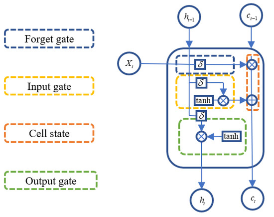
Figure 1.
Structure of an LSTM Cell.
At each time step , the operations within an LSTM cell are as follows:
Specifically, the LSTM uses three gates—forget, input, and output—to modulate information traversal through the cell state. At each time step , the forget gate decides which parts of the previous memory should be retained; the input gate and candidate cell state determine what new information is added; and the output gate controls how much of the updated cell state contributes to the hidden output . The mathematical formulation of these operations is expressed as follows:
where is the sigmoid activation function; denotes the weight matrix of the forget gate; is the hidden state from the previous time step; is the input at the current time step; is the bias term; is the previous cell state, denotes the portion of the state that is forgotten, and represents the new information added to the cell state.
In on-machine measurement scenarios, error data typically exhibit strong temporal dependencies. LSTM networks are capable of modeling the nonlinear evolution between historical and current errors, thereby enabling dynamic prediction.
The LSTM structure can effectively retain critical states from historical measurements and filter out short-term noise disturbances, providing a more accurate basis for real-time error prediction. However, conventional LSTM networks are unidirectional, relying solely on past information and therefore unable to capture potential influences from future states. To overcome this limitation, we employ a Bi-LSTM that learns temporal dependencies in both directions, as illustrated in Figure 2.
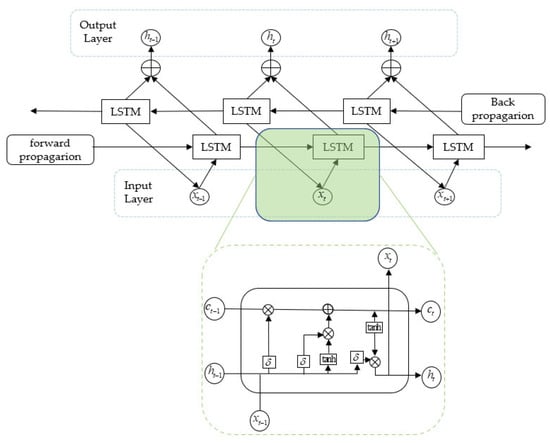
Figure 2.
Bi-LSTM network diagram.
The Bi-LSTM architecture consists of two parallel LSTM networks: one processes the input sequence in the forward direction, while the other processes a time-reversed version of the sequence in the backward direction. The outputs from both directions are then combined to form the final representation at each time step, thereby enhancing the model’s ability to capture complex temporal structures. The output representation at time step can be expressed as follows:
where is the hidden state from the forward LSTM, is the hidden state from the backward LSTM, denotes the concatenation operation.
This bidirectional structure enables the model to exploit both past and future contextual information, improving the accuracy of sequential error prediction in on-machine measurement tasks.
Although Bi-LSTM enhances the modeling performance, its network structure is relatively complex, involving a larger number of parameters. This results in longer training times and a higher risk of falling into local optima or overfitting. To address these challenges, this study further introduces the WOA to perform global optimization of key hyperparameters in the Bi-LSTM model, such as learning rate, number of hidden units, and batch size. The objective is to improve training efficiency and generalization capability, thereby further enhancing the accuracy and robustness of error prediction.
3.4. Whale Optimization Algorithm for Hyperparameter Optimization
Why WOA? Hyperparameter tuning here is a black-box optimization over a mixed discrete–continuous space, where the objective is the validation RMSE after training with early stopping. This objective is non-differentiable, often multi-modal, and noisy. The WOA is well-suited: its population-based encircling/spiral/random moves balance exploration and exploitation on non-convex landscapes; it has few control parameters, easing configuration compared with GA/PSO; it accommodates mixed variables via feasibility mapping; and it parallelizes training-based fitness evaluations under a fixed computed budget. We therefore adopt WOA to select the CNN–Bi-LSTM hyperparameters; implementation details are provided in this subsection.
Other popular metaheuristic optimizers for hyperparameter tuning include Particle Swarm Optimization (PSO) and Genetic Algorithm (GA), which have been widely adopted due to their simplicity and convergence efficiency [33,34].
PSO mimics the collective behavior of bird flocking or fish schooling, while GA evolves candidate solutions through crossover and mutation operations inspired by natural selection.
However, both methods may easily fall into local optima when dealing with highly nonlinear or multi-modal search spaces, motivating the use of the Whale Optimization Algorithm (WOA) for better global exploration.
WOA was first proposed by Mirjalili and Lewis in 2016, inspired by the bubble-net hunting strategy of humpback whales [35]. The algorithm features a simple structure, ease of implementation, and strong global search capability. It simulates the prey-hunting behavior of whales through three main mechanisms: encircling prey, spiral bubble-net attacking, and random search. These mechanisms enable WOA to effectively balance exploration and exploitation during the optimization process, thereby helping the prediction model to achieve better convergence and generalization performance.
3.4.1. Encircling Prey
Humpback whales are capable of identifying the position of their prey and encircling it cooperatively.
In the Whale Optimization Algorithm (WOA), this hunting behavior is mathematically abstracted to describe how the population converges toward the current best candidate solution.
Each whale represents a search agent with a position vector in the solution space at iteration , while the best position found so far is denoted as and regarded as the prey.
The distance vector quantifies how far each whale is from the prey and determines the direction of movement toward it. Accordingly, the encircling mechanism can be formulated as follows:
where
and denote the positions of the current whale and the best whale (prey) at iteration , respectively;
represents the updated position of the whale in the next iteration;
and are coefficient vectors controlling convergence behavior; and is the absolute distance between each whale and the prey in the search space.
The coefficient vectors and are further defined as follows:
Here, are random vectors that introduce stochasticity into the search process, and decreases linearly from 2 to 0 over the course of iterations to gradually shift the algorithm’s behavior from global exploration to local exploitation.
Through this adaptive mechanism, whales dynamically adjust their positions relative to the best solution, effectively modeling the natural encircling behavior observed in humpback whale hunting.
3.4.2. Bubble-Net Attacking
This behavior includes two strategies: shrinking encircling and spiral updating:
- (1)
- Shrinking Encircling: By decreasing the absolute value of the coefficient vector , the search range narrows to , allowing whales to tighten the encircling loop around the prey.
- (2)
- Spiral Updating Position: The position is updated in a logarithmic spiral form as follows:
- (3)
- Search for Prey: When , the whale randomly selects another individual instead of the best solution, encouraging population diversity and preventing premature convergence:
Through the above improvements to the WOA, this study achieves efficient hyperparameter tuning and global optimal solution exploration for the CNN-Bi-LSTM model. The resulting parameter configurations provide a stable and robust foundation for the error prediction model, thereby further enhancing its prediction accuracy and generalization performance.
3.5. WOA-CNN-Bi-LSTM Prediction Model
To enhance the prediction accuracy of machining errors in on-machine measurement (OMM) scenarios, this study proposes a hybrid prediction model that integrates the Whale Optimization Algorithm (WOA) with a Convolutional Bidirectional Long Short-Term Memory network (CNN-Bi-LSTM). Structurally, the model combines the local feature extraction capability of CNN with the bidirectional temporal modeling ability of Bi-LSTM, while WOA is employed to optimize hyperparameters automatically. In this way, the model achieves both the strong representational power of deep learning and the adaptive search capability of meta-heuristic optimization. The overall framework is illustrated in Figure 3.
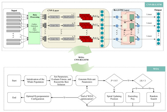
Figure 3.
The overall architecture and optimization process of the integrated CNN-Bi-LSTM model with the WOA.
Figure 3 depicts the end-to-end pipeline. Top block (CNN–Bi-LSTM): time-aligned on-machine measurement (OMM) signals are processed in the Data Processing unit and segmented into windows to form an input tensor of shape (1000, 20, 1, 1) (batch size, height, width, channels). For 1-D convolutions, this is equivalent to [1000, 1, 20] after squeezing the last axis. The windows enter a Conv1D-MaxPool1D-ReLU stack that learns local temporal patterns; the resulting feature maps are passed to a Bi-LSTM layer group to capture long-range dependencies. The output head maps the final representation to the target (regression, linear activation). The turquoise double arrow labeled “WOA–CNN-Bi-LSTM” indicates that the lower optimizer tunes the hyperparameters of this network.
Bottom block (WOA): The Whale Optimization Algorithm searches hyperparameters—including the number of convolutional layers, kernel size and filters per layer, the number of Bi-LSTM layers and hidden units, dropout rate, learning rate, batch size, and search meta-parameters (population size, maximum iterations). The flow begins with initialization of the whale population, proceeds with coefficient updates, candidate generation via encircling/exploration/spiral moves, and fitness evaluation on the validation set, and repeats until the maximum iteration or convergence; the best hyperparameter configuration is returned.; each candidate is trained and evaluated, the fitness is recorded, and the current best solution is kept (elitism). The Generate Relevant Parameters box updates the control variables and distance measures; decisions follow the standard WOA rules: if and the algorithm performs Encircling Prey (exploitation); if and it performs Random Search (exploration); otherwise it executes Spiral Updating Position toward the current best. The loop continues until the End of WOA optimization is satisfied, then outputs the Optimal hyperparameter configuration, which is applied to the top network.
For reproducibility and parameter tuning, the hyperparameters involved in the model are categorized into two groups: structural hyperparameters of the CNN-Bi-LSTM network and optimization meta-parameters of WOA. The former determines the representational capacity and temporal modeling depth of the network, while the latter defines the population size, iteration number, and update strategies of WOA, directly affecting convergence speed and global search ability. The specific settings of these two categories are summarized in Table 1 and Table 2.

Table 1.
Search ranges used by WOA for hyperparameter optimization.
Table 2.
Final optimal hyperparameter settings selected by WOA.
For clarity and reproducibility, we report both the search ranges used by the Whale Optimization Algorithm (WOA) and the final optimal hyperparameters selected after convergence.
Table 1 lists the predefined ranges within which WOA automatically tuned each hyperparameter. During optimization, WOA updated candidates via its encircling, spiral, and random-search mechanisms, using validation RMSE as the fitness function with a fixed random seed.
The final settings chosen by WOA are presented in Table 2.
3.6. Evaluation Indicator
To provide a comprehensive and objective evaluation, we report four standard metrics—RMSE, MAE, MAPE, and R2—which jointly quantify absolute and relative error as well as goodness of fit.
where is the true value, is the predicted value, is the number of samples, and the overline symbol denotes the arithmetic mean of all actual values.
The combination of these evaluation metrics compensates for the limitations of using a single metric and provides a more objective and comprehensive assessment of the error prediction performance. Specifically, RMSE is sensitive to large errors and can effectively identify abnormal predictions; MAE better reflects the overall error level by avoiding the over-amplification of outliers; MAPE standardizes the error magnitude, making it suitable for performance comparison across different models; and R2 offers an overall measure of model fit. Although R2 may have certain limitations when used alone, in combination with the aforementioned error metrics, it enables a more complete evaluation of the model’s prediction accuracy and robustness.
4. Results
To rigorously assess the effectiveness of the proposed WOA-CNN-Bi-LSTM prediction model in the context of OMM error prediction, this chapter conducts a series of experiments and analyses based on a specific machining case. Firstly, an OMM experimental platform for the central casing of a gas turbine is established, from which real machining error data is collected and subjected to systematic cleaning and preprocessing, ensuring the representativeness and consistency of input samples. Based on this, performance evaluation proceeds along three levels: First, a comparison of different network architectures is performed to clarify the contribution of convolutional encoding and bidirectional temporal modeling in capturing complex error patterns. Second, multiple meta-heuristic optimization algorithms are introduced to search for and validate the optimal hyperparameter configuration of CNN-Bi-LSTM, comparing the convergence behavior and prediction accuracy across different strategies. Third, robustness analysis is conducted to assess the generalization performance and stability of the final WOA-CNN-Bi-LSTM model under varied data distributions and machining conditions. Through this validation framework, the chapter aims to systematically demonstrate the rationality and effectiveness of the proposed method from multiple perspectives, including case construction, model comparison, optimizer evaluation, and generalization analysis.
4.1. Case Establishment and Data Acquisition
Before conducting model performance verification, it is essential to rely on a specific machining case to obtain representative data samples. Establishing such a case not only provides on-machine measurement data that reflect real operating conditions but also helps ensure the reliability and reproducibility of model training and testing. To this end, this study selected the central casing of a gas turbine as the research object and constructed the corresponding experimental platform, enabling the acquisition of high-precision error data during actual machining. The following subsection presents a detailed description of the workpiece and experimental platform.
4.1.1. Workpiece and Experimental Platform
In this study, the central casing of a gas turbine was selected as the workpiece. As a representative thin-walled component with a complex geometry, its dimensional accuracy and surface quality are critical to the overall performance of the engine, making it an ideal object for validating the proposed OMM prediction model. The experiments were carried out on a Cincinnati vertical four-axis machining center equipped with a Siemens 840D CNC system (Munich, Germany) and a Renishaw OMP60 touch probe (Wotton-under-Edge, UK), as shown in Figure 4 and Figure 5. This configuration enables fully automated on-machine measurement cycles, allowing real-time acquisition of surface positional errors during machining. Compared with conventional offline inspection, the approach significantly reduces clamping-induced deviations and measurement delays, thereby improving the authenticity and timeliness of the collected data.
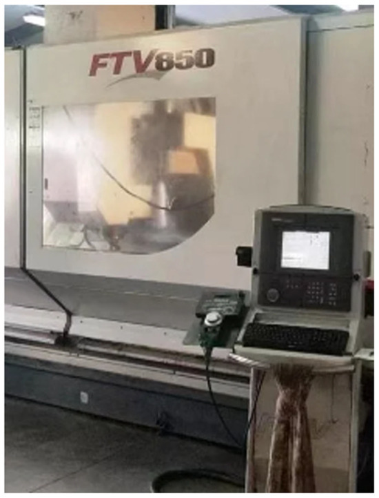
Figure 4.
Cincinnati vertical four-axis machining center (USA).
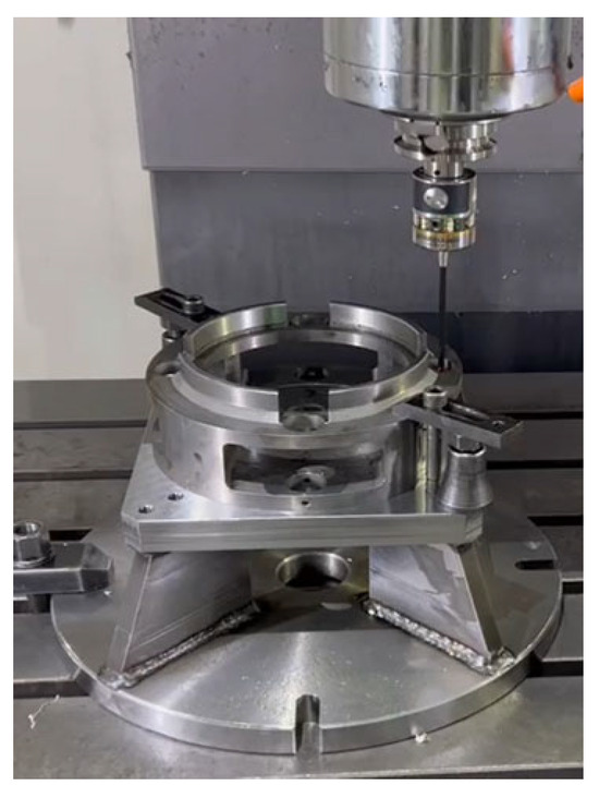
Figure 5.
On-machine measurement process diagram.
Furthermore, all deep learning model training and validation procedures were conducted on a high-performance workstation. The system was configured with an Intel i7-10870 CPU (Santa Clara, CA, USA) and an NVIDIA GeForce RTX 3070 GPU (Santa Clara, CA, USA), providing sufficient computational resources for large-scale data processing and complex neural network training, and ensuring robust support for subsequent experiments.
4.1.2. Data Acquisition and Processing Procedure
In this study, an OMM system was employed during machining to perform real-time inspection of key surface features, ensuring continuous and dynamic acquisition of error information. To ensure the validity and consistency of the input samples, the raw data underwent a series of preprocessing steps prior to modeling. Specifically, obvious outliers were removed to eliminate extreme points that could bias model training; noise smoothing was applied to reduce fluctuations originating from the measurement system; and all error features were standardized to eliminate differences in units and magnitudes, thereby preventing certain features with large values from dominating model weights. This process not only improved data balance but also accelerated the convergence speed and stability of the deep learning models.
After preprocessing, 1000 valid samples were obtained for each of the two workpieces. The entire dataset was randomly split into three subsets—56% for training, 14% for validation, and 30% for testing—to ensure sufficient independent samples for model selection and final evaluation.
Within the training portion, 20% of the data was further separated as a validation subset, which was used exclusively for hyperparameter tuning and early stopping to prevent overfitting.
The remaining 56% of the data was used for actual parameter learning. All data splitting was performed using a fixed random seed to guarantee reproducibility.
This three-way split (training/validation/testing = 56%/14%/30%) ensures reliable performance estimation and consistent convergence during the optimization process.
4.2. Model Performance Evaluation
To comprehensively assess the effectiveness of the proposed WOA-CNN-Bi-LSTM model on real-world OMM data from a gas turbine casing, this section aims to answer two key questions: (1) what to learn—whether the CNN–Bi-LSTM architecture provides substantial advantages over simplified baselines such as LSTM, Bi-LSTM, and CNN-LSTM in modeling OMM error patterns—and (2) how to learn—whether different hyperparameter optimizers (e.g., WOA, GA, PSO, random search) significantly influence model convergence behavior and generalization capability. To this end, the section is organized into three parts: first, a structural comparison (Section 4.2.2) that contrasts CNN-Bi-LSTM with its simplified counterparts under identical preprocessing and training setups to verify the benefits of convolutional feature extraction and bidirectional temporal modeling; second, an optimizer comparison (Section 4.2.3) that evaluates how different global search strategies affect performance stability; and finally, a summary of combined results and robustness analysis (Section 4.2.4) to validate the model’s practical feasibility across heterogeneous machines and under real-time constraints.
4.2.1. Architecture Comparison (What to Learn)
This subsection explores the question of “what to learn” when designing prediction architectures for OMM error data. To address this, we conduct a comparative evaluation under uniform preprocessing and training settings, assessing the proposed CNN–Bi-LSTM model against both temporal and non-temporal baselines. The temporal group includes unidirectional LSTM, bidirectional Bi-LSTM, and CNN-LSTM, while the non-temporal group consists of XGBoost, Random Forest, and GRU—three widely adopted alternatives in industrial prediction tasks. The primary aim is to investigate whether the integration of convolutional operations and bidirectional temporal modeling enhances prediction accuracy and generalization. The comparative results help clarify which architectural choices better support real-time error compensation and intelligent quality control in precision machining environments. Detailed outcomes are visualized in Figure 6.
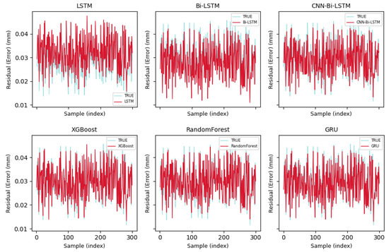
Figure 6.
Prediction performance of all models over the final 30% time segment of the test set.
To more thoroughly assess model performance on the task of error prediction for on-machine measurement (OMM), Figure 6 illustrates the prediction outputs versus ground truth over the final 30% of the test set across six models. Although all models capture the general trend to varying extents, differences emerge in local response sensitivity, spike handling, and systematic bias. Notably, recurrent models such as Bi-LSTM and CNN-Bi-LSTM—especially with their incorporation of bidirectional memory and convolutional feature extractors—demonstrate superior stability and trajectory tracking compared to non-recurrent baselines, suggesting architectural benefits.
Still, visual inspection of predicted curves alone does not fully expose the extent of model bias or generalization robustness. Thus, we further present residual error plots for each model under the same test segment, accompanied by ±1.96 standard deviation bands that represent 95% confidence intervals. As shown in Figure 7, these charts provide quantitative evidence of error volatility, outlier dispersion, and model reliability for downstream decision-making.
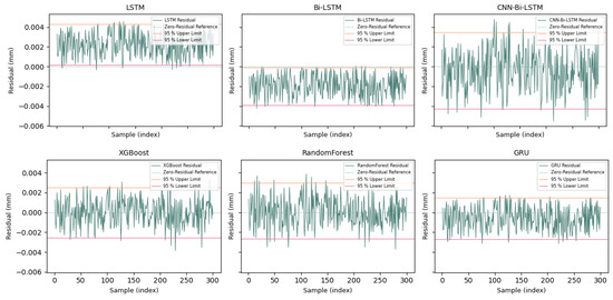
Figure 7.
Residual error sequences with ±1.96 confidence interval across models.
The residual error sequences of six representative models, evaluated on the final 30% segment of the test set, are illustrated in Figure 7. Among these, the top row displays three recurrent neural network variants. In each sub-figure, the residual curve is depicted in green, accompanied by ±1.96 standard deviation bounds shown as pink lines, which represent the 95% confidence interval. A red line indicates zero-residual reference across all subplots.
The CNN-Bi-LSTM model demonstrates tighter residual distribution and lower oscillation, with most predictions falling well within the confidence band, indicating robust generalization. In contrast, models like LSTM and GRU exhibit wider and more erratic deviations, suggesting greater instability or inherent bias. Tree-based methods such as Random Forest and XGBoost show relatively stable trends but occasionally deviate from the center line.
To further enhance performance for practical error compensation in industrial environments, the next section explores the integration of three nature-inspired optimization strategies—WOA, GA, and PSO—into the CNN-Bi-LSTM architecture. Their effects on parameter tuning, prediction accuracy, and runtime efficiency will be thoroughly evaluated, providing valuable insights for model selection and deployment in on-machine measurement scenarios.
4.2.2. Optimizer Evaluation (How to Learn)
To address the core question of “how to learn,” this subsection systematically compares three representative metaheuristic optimization algorithms—WOA, Particle Swarm Optimization (PSO), and Genetic Algorithm (GA)—within a unified CNN-Bi-LSTM framework, all of which have been successfully applied in hyperparameter optimization and time-series prediction tasks. All experiments were conducted under identical dataset splits and training epochs to ensure comparability and fairness.
During the experiment, we first fixed the network structure of CNN Bi-LSTM and used the optimizer as the unique variable to train and validate it for 200 epochs. The objective of optimization is to minimize the mean square error (MSE) and simultaneously track the trends of training loss and validation loss, as shown in Figure 8, to examine the differences in convergence speed, final accuracy, and stability among the three optimizers.
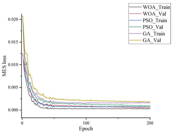
Figure 8.
Comparison of training and validation loss curves using different metaheuristic optimizers in CNN-Bi-LSTM models.
The results indicate that all three optimizers exhibit a sharp error decline within the first 20 epochs, reflecting effective early-stage learning. As training progresses, the loss curves gradually plateau, entering the fine-tuning phase. Among them, WOA achieves the fastest convergence and the lowest final error on both training and validation sets, with the smoothest validation curve and the least volatility, demonstrating superior robustness and repeatability. PSO ranks second, achieving moderate convergence with acceptable stability. GA, however, shows considerable fluctuations in the validation curve during later stages, indicating weaker consistency and sensitivity to initialization.
In summary, WOA is validated as the most effective optimizer in this study. Its rapid convergence, lower final error, and greater stability make it particularly well-suited for high-precision tasks such as real-time OMM error modeling and compensation.
4.2.3. Performance Comparison of Predictive Models
To make cross-metric comparisons more interpretable and to highlight the relative strengths of each model, we normalized all metric values across models. Specifically, each metric was min–max scaled to [0, 1] per column; for error-type metrics (RMSE, MAE, MAPE), values were inverted so that larger scores indicate better performance, while R2 was used directly. The resulting normalized performance scores are visualized as a heat map in Figure 9 (darker green = better). The raw metric values, as well as the exact normalization procedure and the latency metrics (inference time and total computation time), are reported in Table A1 of Appendix A.
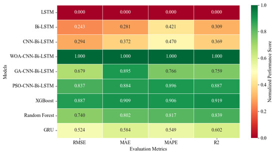
Figure 9.
Heatmap of normalized performance metrics for nine predictive models (higher is better).
As illustrated in Figure 9, the hybrid WOA-CNN-Bi-LSTM model consistently achieved the best accuracy across RMSE, MAE, and MAPE, while also attaining the highest R2 value, confirming its superior error-prediction capability. The optimizer augmented PSO-CNN-Bi-LSTM and GA-CNN-Bi-LSTM models also showed competitive accuracy, though GA’s performance was less stable. Among non-hybrid networks, GRU achieved a slightly better balance between accuracy and speed compared to vanilla LSTM and Bi-LSTM, whereas Random Forest and XGBoost demonstrated strong accuracy but were limited by inference efficiency.
While Figure 9 benchmarks the predictive accuracy of all candidates, practical deployment also hinges on computational efficiency. We therefore report per-model inference time and total training time under the same hardware and implementation settings, enabling an accuracy–efficiency trade-off analysis. The results are summarized in Figure 10 (log scale), where “Total Time” refers to the single-run training time of the final model at its optimal hyperparameters, excluding the full meta-heuristic search.
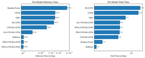
Figure 10.
Comparison of per-model inference time and total computational time across nine machine learning architectures.
Complementary to accuracy, Figure 10 highlights the computational efficiency of the models. XGBoost achieved the shortest inference and total runtime, but at the expense of predictive generalization. In contrast, CNN-Bi-LSTM and its optimizer-enhanced variants delivered both competitive runtime efficiency and significantly higher prediction accuracy, thereby striking a better Pareto balance between accuracy and efficiency.
Overall, these results demonstrate that the CNN-Bi-LSTM framework—especially when integrated with metaheuristic optimizers such as WOA—offers the most effective trade-off for OMM error prediction tasks, combining robust accuracy, efficient training convergence, and manageable computational costs.
4.2.4. Feasibility Validation of the Improved Algorithm
To assess the deployability of the proposed WOA-CNN-Bi-LSTM model in a heterogeneous machine-tool environment, we collected 1000 additional OMM samples from a different machining center. The preprocessing pipeline and the three-way split (training/validation/testing = 56%/14%/30%) were kept identical to ensure consistency across experiments.
To jointly measure model accuracy and efficiency, we evaluated RMSE, MAE, MAPE, and R2, together with inference time and total runtime. To enable clearer cross-model comparison, all metric values were normalized column-wise using min–max scaling, where larger values indicate better performance. The resulting normalized heatmap is shown in Figure 11, and the detailed numerical results are provided in Table A2 of Appendix A.
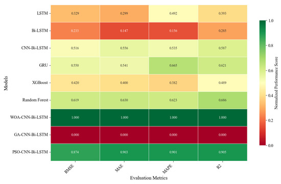
Figure 11.
Normalized heatmap of performance on the cross-machine test set (higher is better).
Figure 11 presents the normalized performance heatmap on the cross-machine dataset. WOA-CNN-Bi-LSTM attains near-unity scores across all four metrics, outperforming GA-/PSO-optimized and non-optimized CNN-Bi-LSTM as well as LSTM/Bi-LSTM, GRU, XGBoost, and Random Forest. This confirms that WOA’s global hyperparameter search consistently finds better configurations under distribution shifts, yielding systematic error reductions. Quantitatively, compared with the LSTM baseline, RMSE and MAE drop by 35% and 38%, respectively; relative to the non-optimized CNN-Bi-LSTM, RMSE is still 28% lower, demonstrating clear gains even in cross-equipment scenarios.
While Figure 11 focuses on cross-machine predictive accuracy, practical deployment also depends on the computational efficiency of each model. To comprehensively evaluate real-world applicability, we further compared the inference latency and total training time of all architectures under identical hardware and configuration settings. The results, summarized in Figure 12, reveal how each model balances predictive performance against computational cost.
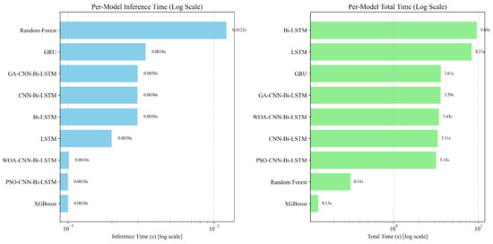
Figure 12.
The inference time and total training time of different models across machine tools.
Figure 12 shows inference and total times. For inference, WOA-CNN-Bi-LSTM is on par with PSO-CNN-Bi-LSTM and XGBoost, substantially faster than GRU/Bi-LSTM/CNN-Bi-LSTM and Random Forest. For total runtime, WOA-CNN-Bi-LSTM forms a competitive cluster with CNN-Bi-LSTM/PSO/GA and is much faster than LSTM/Bi-LSTM. In the accuracy–time trade-off, WOA-CNN-Bi-LSTM lies on the Pareto frontier, achieving state-of-the-art accuracy with near-fastest inference. XGBoost is the fastest but less accurate; Random Forest trains quickly yet infers slowly, making it less suitable for real-time compensation.
In terms of robustness, WOA-CNN-Bi-LSTM exhibits consistently strong and less volatile results than PSO/GA on the cross-machine test set, evidencing better generalization and noise tolerance—both essential for on-machine error prediction. Overall, WOA-CNN-Bi-LSTM simultaneously satisfies high-accuracy and high-efficiency requirements and is technically feasible for industrial deployment.
5. Discussion
This study evaluates OMM error prediction along two axes—what to learn (architecture) and how to learn (optimizer).
CNN-Bi-LSTM outperforms LSTM and Bi-LSTM across all four accuracy metrics. The reason lies in CNN’s capability of extracting stable local structural patterns from raw sequences, while Bi-LSTM enhances the modeling of long-term dependencies through bidirectional memory. The complementarity between the two enables more discriminative and noise-resilient feature representations.
Within the same backbone, WOA-CNN-Bi-LSTM surpasses PSO and GA based variants. Its advantage is reflected in faster early-stage error reduction, lower final validation error, and reduced oscillation amplitude. This stems from WOA’s three-stage mechanism—encircling, spiral updating, and stochastic search—which ensures global exploration in the early phase and enhances convergence and fine-tuning in later phases, thereby mitigating the risk of premature convergence.
While maintaining high prediction accuracy, WOA-CNN-Bi-LSTM achieves millisecond-level inference latency and acceptable overall training time. Compared with tree-based models, the computational cost is slightly higher, but it maintains a superior position in accuracy–time, making it suitable for real-time compensation and closed-loop control tasks.
Experiments on heterogeneous machine-tool datasets confirm that WOA-CNN-Bi-LSTM retains significant improvement compared to non-optimized CNN-Bi-LSTM and conventional baselines. This indicates that global hyperparameter search via WOA can effectively mitigate distribution shifts caused by equipment heterogeneity, thereby providing better cross-platform transferability.
Limitations and Threats: (a) Data sources remain limited to representative parts and machining conditions, leaving potential risks in out-of-distribution scenarios; (b) Although meta-heuristic search improves efficiency, it is still computationally sensitive in large search spaces; (c) Model interpretability remains limited, and stronger mapping between “error sources–features–predictions” is needed.
Engineering Implications: (a) For production lines sensitive to real-time performance, a lightweight CNN-Bi-LSTM combined with staged WOA is recommended to shorten tuning time. (b) For cross-machine deployment, domain adaptation, parameter finetuning, and online calibration are advisable. (c) For quality traceability, integrating uncertainty estimation and anomaly detection modules can enhance interpretability and maintainability.
6. Conclusions
This research introduces a hybrid CNN-Bi-LSTM model optimized by the Whale Optimization Algorithm (WOA) for real-time error prediction in on-machine measurements (OMMs) within complex manufacturing environments. Based on systematic experiments involving real-time measurement data from gas turbine central casing machining processes, the following key conclusions have been drawn:
- (1)
- The proposed CNN–Bi-LSTM–WOA hybrid model outperforms the baseline LSTM across all metrics, reducing RMSE by 53.58%, MAE by 54.96%, MAPE by 57.65%, and increasing R2 by 11.17%. These quantitative results confirm the model’s capability to effectively capture intricate nonlinear error patterns.
- (2)
- The hybrid architecture strategically integrates CNN’s localized feature extraction strengths with Bi-LSTM’s advanced modeling of long-term sequential dependencies, enabling multi-scale and multi-level feature fusion. This synergistic approach notably enhances the representation of non-stationary error patterns and complex dynamic behaviors, ensuring stable and highly accurate predictive outcomes.
- (3)
- The implementation of the Whale Optimization Algorithm (WOA) provides efficient global hyperparameter optimization capability. Compared with Genetic Algorithm (GA) and Particle Swarm Optimization (PSO), WOA demonstrates superior global search performance and faster convergence, significantly enhancing the model’s generalization capabilities and practical accuracy.
- (4)
- Validation through real-world machining experiments demonstrates that the proposed CNN-Bi-LSTM-WOA model offers excellent real-time responsiveness and practical applicability in an industrial setting, effectively minimizing actual dimensional deviations during machining processes. This provides significant theoretical and technical support for online measurement, intelligent feedback control, and optimization of advanced manufacturing processes.
In summary, this study successfully develops an efficient and accurate method for real-time error prediction in OMM, achieving substantial advancements in both theoretical innovation and practical engineering applications. Future research will emphasize further improvements in data preprocessing and feature engineering, investigate lightweight and embedded implementation approaches, and enhance model robustness and generalization under increasingly complex machining conditions to continue advancing intelligent manufacturing technologies.
Author Contributions
Methodology, writing—review and editing Z.Z. and H.Q.; software, Y.X.; data curation, X.X.; Format review, F.X.; visualization, C.D.; funding acquisition, H.Q. All authors have read and agreed to the published version of the manuscript.
Funding
This research was funded by Xi’an Municipal Bureau of Science and Technology Program (grant number: 24GXPT0001), Shaanxi Provincial Key R&D Program Projects (grant number: 2023-CX-PT-48) , Shaanxi Province Innovation Capacity Support Program (grant number: 2022GHJD-14)and Shaanxi Provincial Natural Science Basic Research Plan Project (grant number: 2025JC-YBMS-627).
Data Availability Statement
The data that support the findings of this study are available from the corresponding author upon reasonable request.
Conflicts of Interest
The authors declare no conflict of interest.
Appendix A
Table A1.
Prediction performance of different models on machine tool datasets.
Table A1.
Prediction performance of different models on machine tool datasets.
| Indicator | RMSE | MAE | MAPE | R2 | Inference Time (s) | Total Time (s) | |
|---|---|---|---|---|---|---|---|
| Model | |||||||
| LSTM | 0.002530 | 0.002228 | 8.548928 | 0.875408 | 0.00347 | 14.55 | |
| Bi-LSTM | 0.002201 | 0.001884 | 6.476264 | 0.905565 | 0.003304 | 15.99 | |
| CNN-Bi-LSTM | 0.002132 | 0.001772 | 6.233371 | 0.911498 | 0.002493 | 4.96 | |
| WOA-CNN-Bi-LSTM | 0.001174 | 0.001003 | 3.620215 | 0.973147 | 0.001004 | 5.43 | |
| GA-CNN-Bi-LSTM | 0.001609 | 0.001132 | 4.775915 | 0.94957 | 0.001432 | 5.44 | |
| PSO-CNN-Bi-LSTM | 0.001395 | 0.001145 | 4.130406 | 0.962106 | 0.001014 | 5.34 | |
| XGBoost | 0.001327 | 0.001115 | 4.083647 | 0.965247 | 0.001014 | 1.55 | |
| Random Forest | 0.001526 | 0.001246 | 4.521238 | 0.957418 | 0.00553 | 2.13 | |
| GRU | 0.001819 | 0.001512 | 5.842341 | 0.934204 | 0.00345 | 7.35 | |
Table A2.
Prediction performance of different models on the heterogeneous machine-tool dataset.
Table A2.
Prediction performance of different models on the heterogeneous machine-tool dataset.
| Indicator | RMSE | MAE | MAPE | R2 | Inference Time (s) | Total Time (s) | |
|---|---|---|---|---|---|---|---|
| Model | |||||||
| LSTM | 0.015053 | 0.012447 | 7.475883 | 0.905348 | 0.001994 | 8.37 | |
| Bi-LSTM | 0.015807 | 0.01347 | 9.059831 | 0.895623 | 0.002994 | 9.6 | |
| CNN-Bi-LSTM | 0.01359 | 0.010729 | 7.275699 | 0.922852 | 0.002996 | 3.31 | |
| GRU | 0.01332 | 0.010831 | 6.662785 | 0.925882 | 0.0034 | 3.61 | |
| XGBoost | 0.014346 | 0.011775 | 7.996228 | 0.914029 | 0.000997 | 0.13 | |
| Random Forest | 0.01278 | 0.010231 | 6.858793 | 0.93177 | 0.012161 | 0.31 | |
| WOA-CNN-Bi-LSTM | 0.009788 | 0.007752 | 5.083638 | 0.959977 | 0.001013 | 3.45 | |
| GA-CNN-Bi-LSTM | 0.01764 | 0.014453 | 9.792767 | 0.87002 | 0.002998 | 3.59 | |
| PSO-CNN-Bi-LSTM | 0.010778 | 0.008402 | 5.549284 | 0.951474 | 0.000997 | 3.18 | |
References
- Jiang, X.; Tong, Z.; Li, D. On-machine measurement system and its application in ultra-precision manufacturing. In Precision Machines; Springer: Berlin/Heidelberg, Germany, 2019; pp. 1–36. [Google Scholar] [CrossRef]
- Gao, W.; Ibaraki, S.; Donmez, M.A.; Kono, D.; Mayer, J.R.R.; Chen, Y.L.; Szipka, K.; Archenti, A.; Linares, J.M.; Suzuki, N. Machine tool calibration: Measurement, modeling, and compensation of machine tool errors. Int. J. Mach. Tools Manuf. 2023, 187, 104017. [Google Scholar] [CrossRef]
- Shi, H.; Ye, X.; Xing, C.; Ding, S. A new theoretical interpretation of measurement error and its uncertainty. Discret. Dyn. Nat. Soc. 2020, 2020, 3864578. [Google Scholar] [CrossRef]
- Li, D.; Wang, B.; Tong, Z.; Blunt, L.; Jiang, X. On-machine surface measurement and applications for ultra-precision machining: A state-of-the-art review. Int. J. Adv. Manuf. Technol. 2019, 104, 831–847. [Google Scholar] [CrossRef]
- Biju, V.G.; Schmitt, A.M.; Engelmann, B. Assessing the influence of sensor-induced noise on machine-learning-based changeover detection in CNC machines. Sensors 2024, 24, 330. [Google Scholar] [CrossRef]
- Li, H.; Zhang, P.; Deng, M.; Xiang, S.; Du, Z.; Yang, J. Volumetric error measurement and compensation of three-axis machine tools based on laser bidirectional sequential step diagonal measuring method. Meas. Sci. Technol. 2020, 31, 055201. [Google Scholar] [CrossRef]
- Liu, P.; Du, Z.; Li, H.; Deng, M.; Feng, X.; Yang, J. A novel comprehensive thermal error modeling method by using the workpiece inspection data from production line for CNC machine tool. Int. J. Adv. Manuf. Technol. 2020, 107, 3921–3930. [Google Scholar] [CrossRef]
- Zhuang, Q.; Wan, N.; Guo, Y.; Zhu, G.; Qian, D. A state-of-the-art review on the research and application of on-machine measurement with a touch-trigger probe. Measurement 2024, 224, 113923. [Google Scholar] [CrossRef]
- Jiang, Y.; Chen, J.; Zhou, H.; Yang, J.; Hu, P.; Wang, J. Contour error modeling and compensation of CNC machining based on deep learning and reinforcement learning. Int. J. Adv. Manuf. Technol. 2022, 118, 551–570. [Google Scholar] [CrossRef]
- Zhu, L.; Hao, Y.; Qin, S.; Pei, X.; Yan, T.; Qin, Q.; Lu, H.; Yan, B.; Shu, X.; Yong, J. On-machine measurement and compensation of thin-walled surface. Int. J. Mech. Sci. 2024, 271, 109308. [Google Scholar] [CrossRef]
- Li, G.; Ning, H.; He, K.; He, X.H. Comprehensive pre-travel error compensation for on-machine measurement of face gear and tooth surface matching method. Chin. J. Sci. Instrum. 2024, 45, 246–258. (In Chinese) [Google Scholar] [CrossRef]
- Gao, F.; Pan, Z.; Zhang, X.; Li, Y.; Zhang, D.Y. Adaptive sampling method for turbofan blades on-machine measurement. Comput. Integr. Manuf. Syst. 2023, 29, 843–851. (In Chinese) [Google Scholar] [CrossRef]
- Miao, H.; Li, C.; Liu, C.; Wang, C.; Zhang, X.; Sun, W. Machined surface prediction and reliability analysis in peripheral milling operations. Int. J. Mech. Sci. 2024, 272, 109193. [Google Scholar] [CrossRef]
- Finkeldey, F.; Saadallah, A.; Wiederkehr, P.; Morik, K. Real-time prediction of process forces in milling operations using synchronized data fusion of simulation and sensor data. Eng. Appl. Artif. Intell. 2020, 94, 103753. [Google Scholar] [CrossRef]
- Lin, Y.C.; Wu, K.D.; Shih, W.C.; Hsu, P.K.; Hung, J.P. Prediction of surface roughness based on cutting parameters and machining vibration in end milling using regression method and artificial neural network. Appl. Sci. 2020, 10, 3941. [Google Scholar] [CrossRef]
- Bai, L.; Xu, F.; Chen, X.; Su, X.; Lai, F.; Xu, J. A hybrid deep learning model for robust prediction of the dimensional accuracy in precision milling of thin-walled structural components. Front. Mech. Eng. 2022, 17, 32. [Google Scholar] [CrossRef]
- Yao, Z.; Fan, C.; Zhang, Z.; Zhang, D.; Luo, M. Position-varying surface roughness prediction method considering compensated acceleration in milling of thin-walled workpiece. Front. Mech. Eng. 2021, 16, 855–867. [Google Scholar] [CrossRef]
- Zhang, Z.; Qi, Y.; Cheng, Q.; Liu, Z.; Tao, Z.; Cai, L. Machining accuracy reliability during the peripheral milling process of thin-walled components. Robot. Comput.-Integr. Manuf. 2019, 59, 222–234. [Google Scholar] [CrossRef]
- Teimouri, R.; Skoczypiec, S. Predictive modeling of roughness change in multistep machining. J. Intell. Manuf. 2024, 35, 3577–3598. [Google Scholar] [CrossRef]
- Wang, J.; Qi, X.; Ma, W.; Zhang, S. A high efficiency 3D surface topography model for face milling processes. J. Manuf. Process. 2023, 107, 74–87. [Google Scholar] [CrossRef]
- Wang, W.; Shao, J.; Jumahong, H. Fuzzy inference-based LSTM for long-term time series prediction. Sci. Rep. 2023, 13, 20359. [Google Scholar] [CrossRef]
- Li, E.; Bedi, S.; Melek, W. Anomaly detection in three-axis CNC machines using LSTM networks and transfer learning. Int. J. Adv. Manuf. Technol. 2023, 127, 5185–5198. [Google Scholar] [CrossRef]
- Dong, S.; Xiao, J.; Hu, X.; Fang, N.; Liu, L.; Yao, J. Deep transfer learning based on Bi-LSTM and attention for remaining useful life prediction of rolling bearing. Reliab. Eng. Syst. Saf. 2023, 230, 108914. [Google Scholar] [CrossRef]
- Gao, P.; Wang, J.; Shi, Z.; Ming, W.; Chen, M. Long-term temporal attention neural network with adaptive stage division (AD-LTAN) for RUL prediction of rolling bearings. Reliab. Eng. Syst. Saf. 2024, 251, 110218. [Google Scholar] [CrossRef]
- Zhang, H.; Zhang, Q.; Shao, S.; Niu, T.; Yang, X. Attention-based LSTM network for rotatory machine remaining useful life prediction. IEEE Access 2020, 8, 132188–132199. [Google Scholar] [CrossRef]
- Nadimi-Shahraki, M.H.; Zamani, H.; Asghari Varzaneh, Z.; Mirjalili, S. A Systematic Review of the Whale Optimization Algorithm: Theoretical Foundation, Improvements, and Hybridizations. Arch. Comput. Methods Eng. 2023, 30, 4113–4159. [Google Scholar] [CrossRef]
- Hou, G.; Gong, L.; Yang, Z.; Zhang, J. Multi-objective economic model predictive control for gas turbine system based on quantum simultaneous whale optimization algorithm. Energy Convers. Manag. 2020, 207, 112498. [Google Scholar] [CrossRef]
- Cui, X.; Zhu, J.; Jia, L.; Wang, J.; Wu, Y. A novel heat load prediction model of district heating system based on hybrid whale optimization algorithm (WOA) and CNN-LSTM with attention mechanism. Energy 2024, 312, 133536. [Google Scholar] [CrossRef]
- Hou, Z.; Zhang, Y.; Liu, Q.; Ye, X. A hybrid machine learning forecasting model for photovoltaic power. Energy Rep. 2024, 11, 5125–5138. [Google Scholar] [CrossRef]
- Sapnken, F.E.; Tazehkandgheshlagh, A.K.; Diboma, B.S.; Hamaidi, M.; Noumo, P.G.; Wang, Y.; Tamba, J.G. A whale optimization algorithm-based multivariate exponential smoothing Grey-Holt model for electricity price forecasting. Expert Syst. Appl. 2024, 255, 124663. [Google Scholar] [CrossRef]
- Zha, W.; Liu, Y.; Wan, Y.; Luo, R.; Li, D.; Yang, S.; Xu, Y. Forecasting monthly gas field production based on the CNN-LSTM model. Energy 2022, 260, 124889. [Google Scholar] [CrossRef]
- Hochreiter, S.; Schmidhuber, J. Long Short-Term Memory. Neural Comput. 1997, 9, 1735–1780. [Google Scholar] [CrossRef] [PubMed]
- Kennedy, J.; Eberhart, R. Particle swarm optimization. In Proceedings of the ICNN’95-International Conference on Neural Networks, Perth, WA, Australia, 27 November–1 December 1995; Volume 4, pp. 1942–1948. [Google Scholar] [CrossRef]
- Holland, J.H.; Mahajan, M.; Kumar, S.; Porwal, R. Adaptation in Natural and Artificial Systems; The University of Michigan Press: Ann Arbor, MI, USA, 1975; pp. 1–5. [Google Scholar]
- Mirjalili, S.; Lewis, A. The Whale Optimization Algorithm. Adv. Eng. Softw. 2016, 95, 51–67. [Google Scholar] [CrossRef]


Disclaimer/Publisher’s Note: The statements, opinions and data contained in all publications are solely those of the individual author(s) and contributor(s) and not of MDPI and/or the editor(s). MDPI and/or the editor(s) disclaim responsibility for any injury to people or property resulting from any ideas, methods, instructions or products referred to in the content. |
© 2025 by the authors. Licensee MDPI, Basel, Switzerland. This article is an open access article distributed under the terms and conditions of the Creative Commons Attribution (CC BY) license (https://creativecommons.org/licenses/by/4.0/).