A Multigranularity Parallel Pyramidal Transformer Model for Ethylene Production Prediction and Energy Efficiency Optimization

Abstract

Ethylene production prediction is crucial for improving energy efficiency and optimizing processes in the petrochemical industry. However, the production process data of ethylene are highly complex, and the interaction relationships between variables vary at different time granularities. Ignoring these feature relationships can affect the accuracy of ethylene prediction. Traditional prediction methods model data at a single time granularity only and fail to effectively extract multigranularity features. Therefore, to address the complex multigranularity time-varying characteristics of ethylene production, a multigranularity parallel pyramidal Transformer (MPPT) model is proposed to capture and integrate features from ethylene production data at multiple time granularities, enabling accurate production prediction and energy efficiency optimization. The MPPT model integrates three key modules: multiscale decomposition (MSD), parallel pyramid Transformer (PPT), and multigranularity fusion (MF). The MSD converts industrial process data into multigranularity formats, while the PPT extracts both local and global interaction features across different time granularities using a parallel pyramid structure. Finally, the MF module fuses these features to establish a mapping for accurate prediction. We conducted comparative prediction experiments on an ethylene industrial production dataset, where the MPPT model achieved the best performance among all compared prediction models, with an MAE and RMSE of 0.006 and 0.1755, respectively. Furthermore, we leveraged the accuracy of MPPT in ethylene production prediction to optimize production inputs, achieving energy efficiency optimization in ethylene production.

1. Introduction

The petrochemical industry plays a vital role in the modern economy which is extensively applied across a range of sectors including energy, chemicals, building materials, and light industries [1]. Ethylene is one of the important basic chemical raw materials in the petrochemical industry whose downstream products account for more than 70% of the total petrochemical products [2]. The ethylene industry is not only an essential component of the national economy but also plays a critical role in driving technological innovation and social development. Given its importance to national development, the ethylene industry is flourishing. The total ethylene production capacity in 2017 increased to 23.21 million tons and the ethylene equivalent consumption grew by up to 10% [3].

However, the rapid growth of ethylene production will lead to a sharp increase in the total energy consumption and carbon emissions of the ethylene industry. Therefore, it is urgent to reduce the energy consumption in the ethylene production process, and realize the sustainable development of the ethylene manufacturing industry. Using neural networks for yield prediction in the ethylene production process [4] is an effective method for optimizing energy efficiency in the chemical production industry. By modeling and forecasting the ethylene production process with neural networks, we can adjust the energy input ratios for ethylene production, thereby enhancing energy utilization efficiency and reducing carbon emissions.

At present, complex chemical process modeling can be divided into two categories with shallow neural network [5] and deep learning [6]. Shallow neural networks process data through an input layer, a small number of hidden layers, and an output layer to realize the mapping relationship between input and output. It has the advantages of simple structure and low computational cost. Classic shallow neural networks include back propagation (BP) network [7], extreme learning machine (ELM) [8], and radial basis function (RBF) [9]. However, traditional shallow neural networks have limited feature extraction capability and are difficult to capture complex nonlinear relationships. At the same time, shallow neural networks are susceptible to noise and lack of generalization ability, which makes it difficult to meet the demand for accurate prediction in industrial production. Deep learning methods, such as convolutional neural network (CNN) and variational autoencoder (VAE), have advantages including powerful feature learning capabilities, strong generalization ability, and the capacity to handle complex tasks. These strengths make deep learning methods particularly well suited for processing complex and unstructured industrial process data. Therefore, deep learning methods have been used to model the industrial production prediction process. However, single-granularity deep learning methods can only capture fixed time-series dependencies. The complex petrochemical processes involve a multitude of variables and intricate temporal relationships at different granularities. Modeling only at a single granularity fails to capture the comprehensive nature of these processes. By simultaneously modeling the interaction between different variables and the temporal variation features at different granularities, a more accurate and holistic model can be constructed. This multigranularity modeling approach is essential as it enables a deeper understanding and more precise prediction of the petrochemical processes.

Therefore, a novel multigranularity parallel pyramid Transformer (MPPT) model is proposed for predicting ethylene production. The MPPT consists of a multiscale decomposition (MSD) module, parallel pyramid Transformer (PPT) module, and multigranularity fusion (MF) module. The MSD decomposes the original input sequences into multigranularity sequences. The interaction relationship between different input variables may change at different granularities. Then, in order to extract the dynamic interaction relationship at different time granularities, the PPT proposes that the lower layer of the pyramid extracts the local interaction features of variables, and the upper layer of the pyramid extracts the global interaction features of variables. Meanwhile, the parallel pyramid structure extracts the multiscale features of different granularity data. Finally, the multiscale features obtained by the PPT are input to the MF to fuse the features at different time granularities, and the mapping from the multiscale features to the predicted output is established. The MPPT is applied to predict the actual ethylene production, which provides a new production forecasting and energy efficiency optimization method for the production in petrochemical industry. In summary, the contributions of this paper are as follows:

(1)

We proposed a novel multigranularity modeling method, named MPPT, which enables more comprehensive feature extraction for industrial process data.

(2)

We conducted time-series prediction comparative experiments on an industrial ethylene dataset. The results showed that MPPT achieved the best performance among all comparison models.

(3)

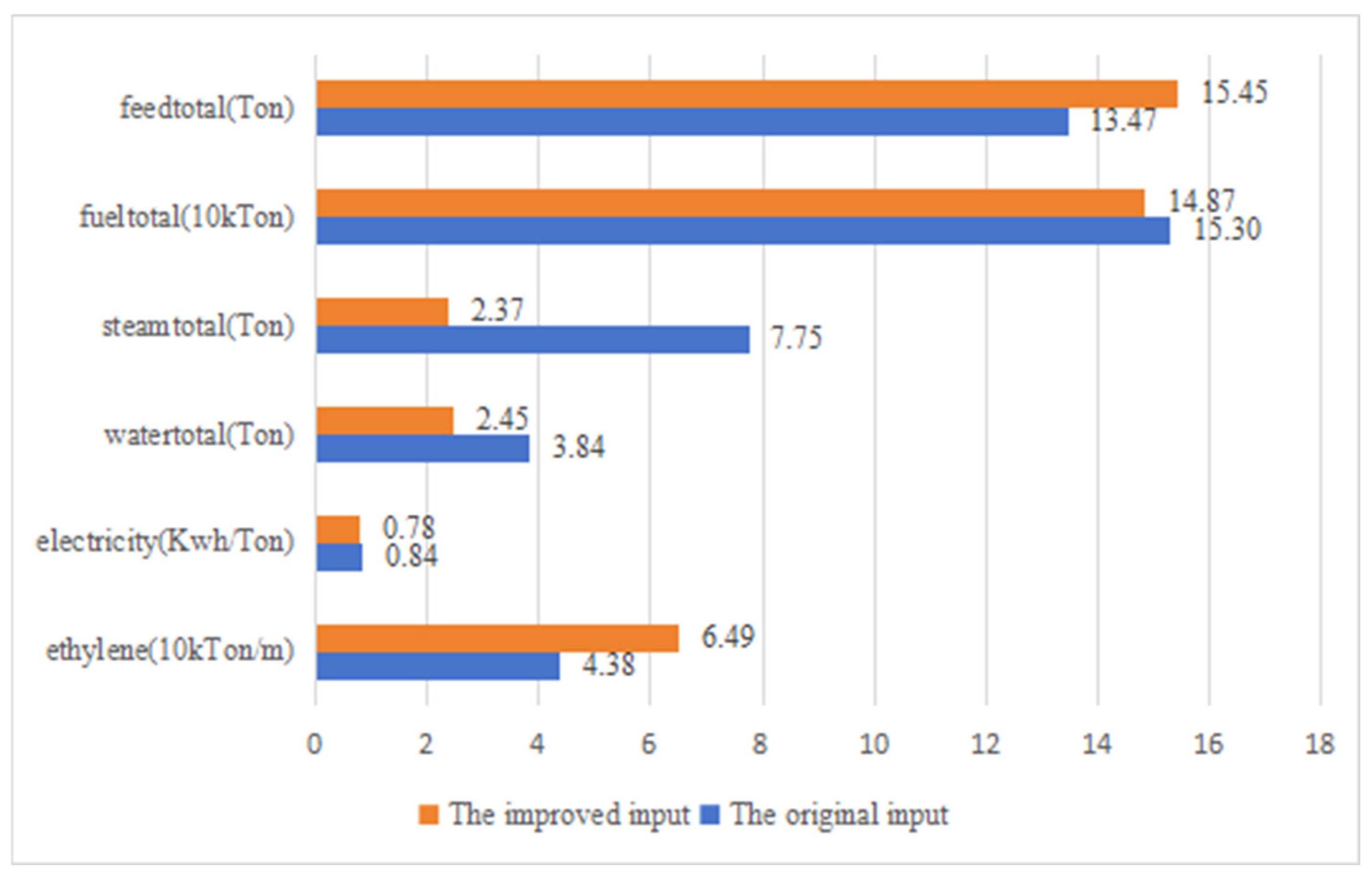
Leveraging the prediction accuracy of the MPPT model for ethylene production, we adjusted and optimized the input ratios in ethylene production, achieving energy efficiency optimization in the ethylene production industry.

2. Related Works

At present, complex chemical process modeling can be divided into two categories with shallow neural network [5] and deep learning [6].

2.1. Shallow Neural Networks

Shallow neural networks realize input–output mapping relationships by processing data through a small number of hidden layers. Classic shallow neural networks include back propagation (BP) network [7], extreme learning machine (ELM) [8], and radial basis function (RBF) [9]. Li et al. [10] used an improved BP neural network to achieve the accurate prediction of changes in energy production and consumption, proving the effectiveness of BP neural networks in the prediction of energy production and consumption. Liang et al. [11] investigated and designed a three-layer BP neural network model applied to the blast furnace coal injection process for predicting the coal ash melting temperature. Xu et al. [12] constructed a combined model for natural gas short-term load prediction based on an improved BP neural network to realize the prediction of natural gas short-term load. However, the traditional BP neural network adopts a gradient descent algorithm for weight updating, which leads to slow convergence speed and makes it easy to fall into local optimal solutions, which affects the performance of the model in practical applications. The ELM is a kind of feed-forward neural network, which improves the problems of slow convergence speed and makes it easy to fall into local optimal solutions of the BP neural network. Han et al. [13] used a new method of combining the ELM and affinity propagation algorithm to forecast ethylene and purified terephthalic acid (PTA) production, which achieved energy saving and emission reduction in production. Ji et al. [14] combined an improved ELM algorithm with the Principal Component Analysis (PCA) method to establish a prediction model of blast furnace gas utilization, which realized the accurate prediction of blast furnace gas utilization. Geng et al. [15] used an innovative model based on ELM and fuzzy C-Means integrating an analytic hierarchy process (FAHP) for petrochemical industry energy consumption prediction, which improved energy utilization and reduced emissions. However, the random initialization of ELM leads to unstable results and limited nonlinear mapping ability, which restricts its application in complex data modeling. The RBF has strong nonlinear mapping ability as well as stability of prediction results, and thus is widely used in practical production. Zhu et al. [16] proposed a radial basis kernel-based ELM for the petrochemical industry modeling of a high-density polyethylene process, which improves the robustness and accuracy of the petrochemical process. Han et al. [17] used an improved RBF model for water quality prediction, which provides a strong support for the optimization of wastewater treatment operations. Mortaza et al. [18] used a multi-objective optimization model combining a fuzzy clustering ranking method with an RBF neural network for the optimization of a hydrogen production process. However, the RBF has high computational complexity and is prone to overfitting, which leads to poor performance in chemical production. Traditional shallow neural networks have limited feature extraction capability and are difficult to capture complex nonlinear relationships. At the same time, shallow neural networks are susceptible to noise and lack of generalization ability, which makes it difficult to meet the demand for accurate prediction in industrial production.

2.2. Deep Learning Methods

Deep learning automatically extracts high-level features through a multilayer structure with stronger complex pattern recognition and nonlinear representation capabilities to effectively handle large-scale data [19]. Geng et al. [3] proposed a cross-feature model based on improved CNN for energy optimization and predictive modeling in the petrochemical industry. Yuan et al. [20] proposed a dynamic convolutional neural network (DCNN) for soft sensor modeling of an industrial hydrocracking process, which improves real-time and prediction accuracy. Shi et al. [21] proposed a combination of sliding window and two-channel CNN to achieve the simultaneous prediction of coal and electricity consumption during cement calcination. Han et al. [22] utilized multiscale VAE regression modeling for the predictive modeling of chemical production processes, which achieves ethylene and propylene process production prediction and energy saving optimization in the production of ethylene and propylene. Jang et al. [23] proposed a feature learning method based on adversarial autoencoder, which ensures the more stable and reliable detection of industrial process faults. Ryno et al. [24] used a deep learning model based on convolutional VAE and multilayer perceptron (MLP) applied to the methane production process to achieve the accurate prediction of multi-physics fields such as temperature and flow rate in the combustor. Although deep learning methods have achieved great improvement in feature extraction compared to traditional shallow neural networks, the complexity of industrial production process data still requires more robust feature representations. Transformer [25] can extract global feature representations, and its self-attention mechanism can extract interrelationships between features without relying on sequence distance. Liu et al. [26] proposed an interpretable Transformer network with data pattern correlation for predictive modeling and critical sample analysis in industrial processes. Han et al. [27] constructed a predictive model for the liquefied petroleum gas industrial production process using the Boruta algorithm based on CNN and Transformer, which improved production efficiency and reduced energy consumption. Liu et al. [28] proposed a Transformer-based hierarchical network for solving problems in multi-rate industrial processes. However, single-granularity deep learning methods can only capture fixed time-series dependencies, which cannot address both long-term dependencies and short-term dynamic features simultaneously.

3. Materials and Methods

In this section, a novel multigranularity parallel pyramid Transformer for complex chemical processes is proposed as an ethylene production prediction. The MPPT consists of MSD, PPT, and MF modules.

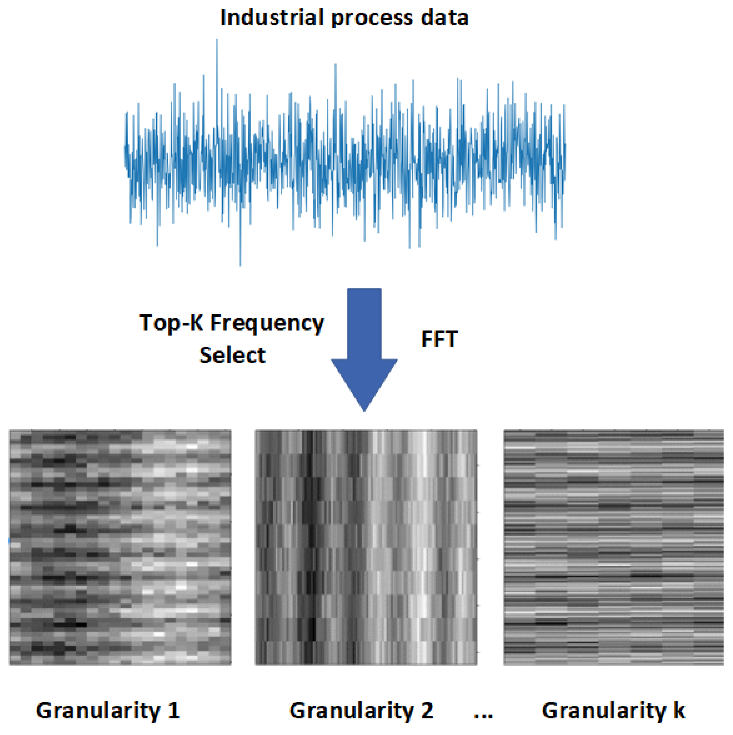
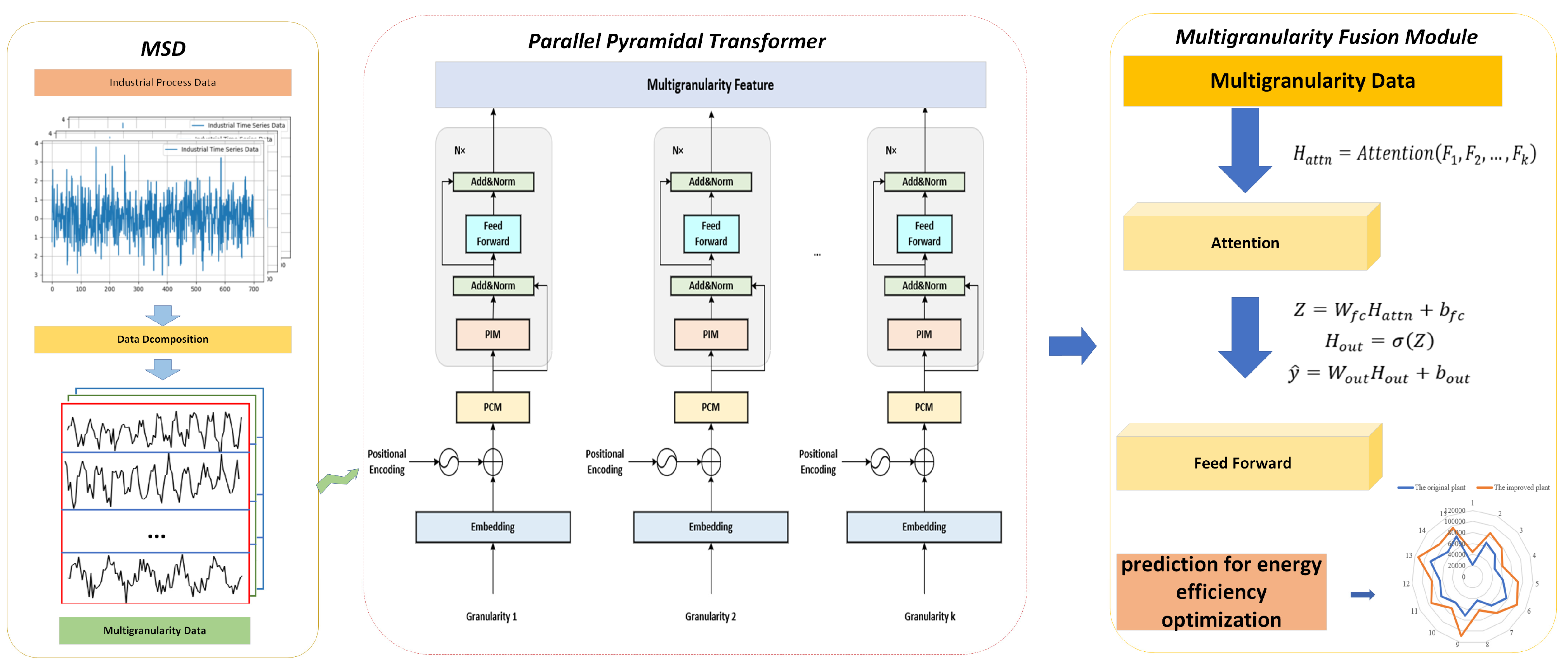
3.1. Multiscale Decomposition Method (MSD)

In complex industrial processes, industrial process data often have complex dynamic characteristics, and the interaction characteristics between variables vary across different time granularities. Extracting these interaction features is crucial for industrial process modeling. For instance, the operating state of production equipment may be affected by different time granularities (short-term oscillations, long-term trends, etc.). At the same time, industrial process data are usually accompanied by noise, which affects the accuracy of prediction models. Traditional methods [11,14,17,20] usually process time series on a single granularity only. However, these methods are weak in feature extraction when dealing with time-series data with complex interactions and cannot extract rich information from different time granularities. To solve this problem, the MSD decomposes the original input sequences into multigranularity sequences. By analyzing multiple cycles, the MSD decomposes time series with complex patterns and reconstructs multigranularity data. As a result, the MSD enables the data to be more intuitively characterized within and between cycles, thus helping the model to extract complex interactions.

First, the input data are mapped to the frequency domain using the Fast Fourier Transform (FFT) method, obtaining the frequency domain representation of the data, as shown in Equation (1):

$$Z_t=\mathrm{F}\mathrm{F}\mathrm{T}\left(X_{input}\right)$$

(1)

where $X_{input}\in {\mathbb{R}}^{L\times N}$ represents the original input, N represents different input variables, and L denotes the length of the time series. After transformation, the input sequence is expressed in the frequency domain, denoted as $Z_t\in {\mathbb{C}}^{F\times N}$. Raw industrial process data are often affected by noise. After applying FFT, low-frequency components, which have the largest amplitudes, represent the main part of the signal. In contrast, high-frequency components often indicate noise or irrelevant information. To address this, we select the K frequencies with the highest amplitudes for computation, where K is a hyperparameter, as shown in Equation (2):

$$F_t=TopK\left(Amp\left(Z_t\right)\right)$$

(2)

Here, $Amp\left(·\right)$ represents the amplitude calculation, and $TopK\left(·\right)$ represents the selection of the K frequencies with the largest amplitudes, $F_t\in {\mathbb{C}}^{K\times N}$ are the filtered K frequencies. By retaining the K frequencies with the largest amplitudes, the main components of the input signal are preserved, while the high-frequency components representing noise are eliminated. Based on the selected K frequencies, the corresponding period lengths are computed, ultimately yielding the reconstructed multigranularity data, as shown in Equation (3):

$$\begin{array}{c}{P}_t=⌈{\displaystyle \frac{L}{F_t}}⌉\\ X=\mathrm{Re}shap{e}_{P_t}(X_{input})\end{array}$$

(3)

where $P_t$ represents the period lengths corresponding to the K frequencies. Using the $\mathrm{Re}shap{e}_{P_t}(\cdot )$, the original input is resampled according to the period lengths $P_t$, ultimately resulting in the multigranularity input $X\in {\mathbb{R}}^{P\times K\times N}$. Here, P denotes the sequence length, K represents the time granularity, and N represents the different variables.

The MSD transforms industrial process data into multigranularity data. This reconstruction allows the data to be characterized more intuitively within and between cycles, aiding the model in extracting complex interactions. Its structure is shown in Figure 1.

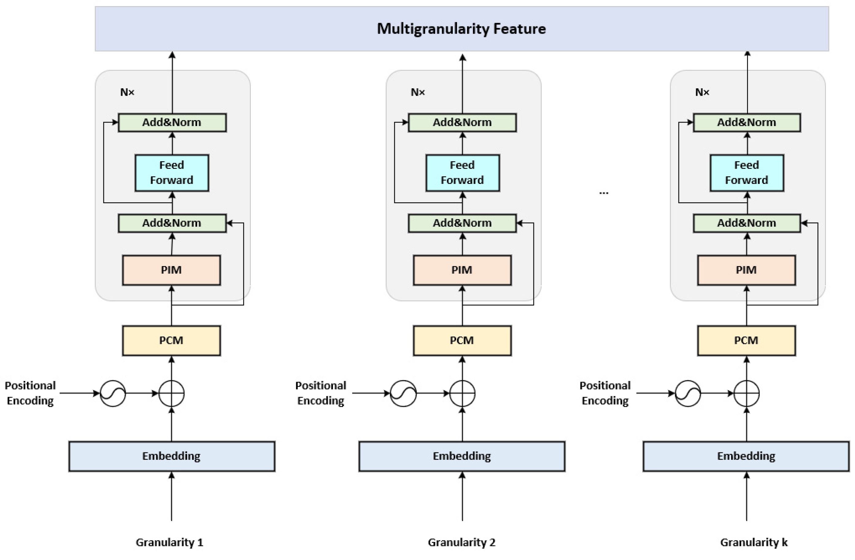
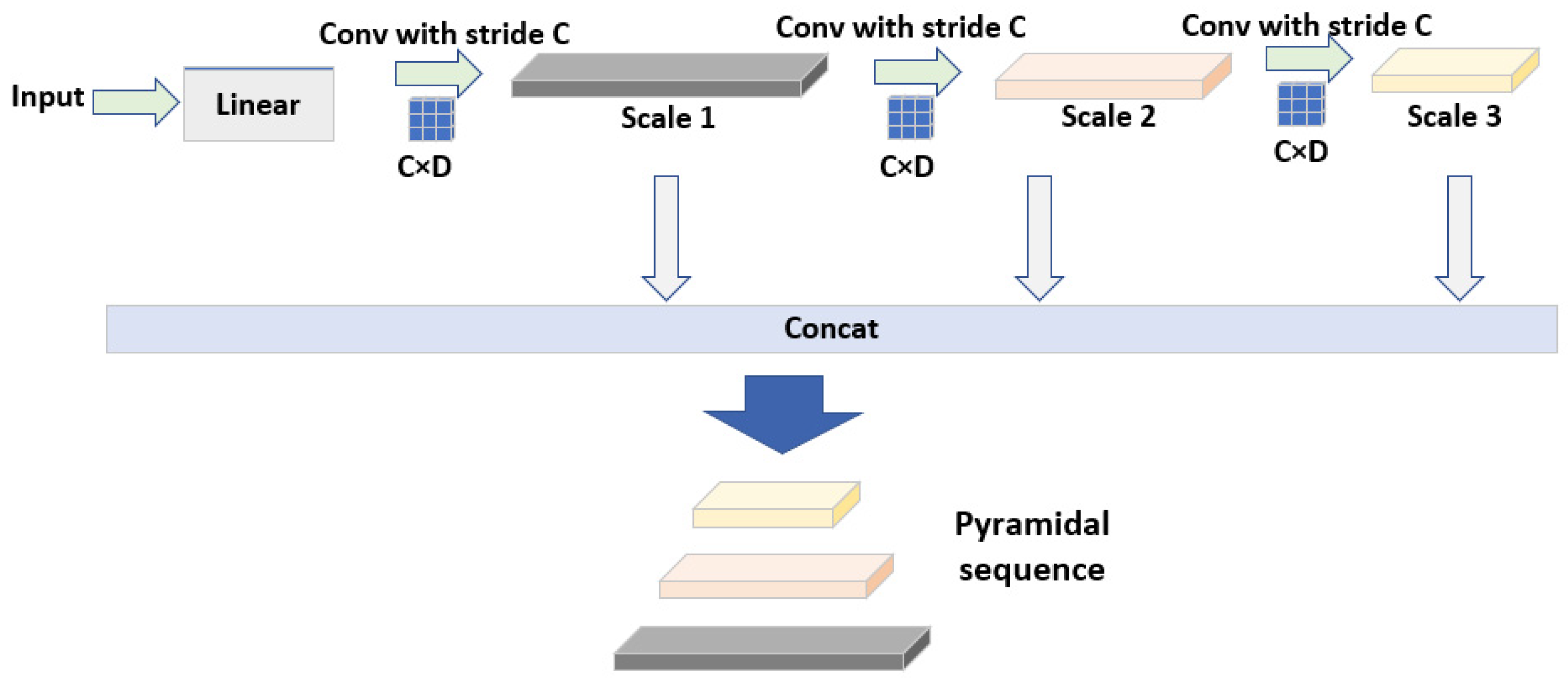
3.2. Parallel Pyramid Transformer (PPT)

In the petrochemical production process, the petrochemical process data are complex and variable. It contains both overall trend direction and local fluctuation changes. Therefore, accurate prediction of petrochemical process data needs to incorporate the dynamic time-varying features of sequences at different time granularities. The PPT extracts the interaction features of sequences at different granularities by modeling the time series at different granularities in parallel. The PPT consists of the Pyramid Construction Module (PCM) and Pyramid Interaction Module (PIM). Based on the inputs of different time granularities, k pyramidal transformer blocks are constructed, which improves on Transformer by adding the PCM and the PIM, as shown in Figure 2.

The PCM is used to initialize the coarse-scale sequences in the pyramid graph so that subsequent PIM modules can exchange information among the nodes in these sequences, as shown in Figure 3. The coarse-scale sequences are constructed by multiple convolution operations. Finally, a C-arys tree can be generated by concatenating the sequences of different scales, as shown in Equations (4)–(7):

$$X^{\prime }=\mathit{Linear}\left(X\right)\in {\mathbb{R}}^{B\times P\times D_k}$$

(4)

$$X^{\left(s\right)}=\mathit{\text{Conv1D}}\left(X^{\left(s-1\right)},\mathit{stride}=C\right)\in {\mathbb{R}}^{B\times \left(P/C^s\right)\times D_k}$$

(5)

$$X_{\mathrm{concat}}=Concat\left[X^{\left(1\right)},X^{\left(2\right)},\dots ,X^{\left(S\right)}\right]\in {\mathbb{R}}^{B\times \sum _{s=1}^S\left(P/C^s\right)\times D_k}$$

(6)

$$X_{\mathrm{output}}={\mathrm{Linear}}_{\mathrm{up}}\left(X_{\mathrm{concat}}\right)\in {\mathbb{R}}^{B\times \sum _{s=1}^S\left(P/C^s\right)\times D}$$

(7)

The input data are first passed through a linear layer, and converted to a new feature dimension $X^{\prime }\in {\mathbb{R}}^{B\times L\times D_k}$, where B is the batch size and D is the dimension. After that, it goes through multiple iterations of convolutional layers with kernel size C to obtain the convolutional result of each layer, $X^{\left(1\right)},X^{\left(2\right)},\dots ,X^{\left(S\right)}$ and then the convolution results are spliced to obtain $X_{\mathrm{concat}}\in {\mathbb{R}}^{B\times \sum _{s=1}^S\left(L/C^s\right)\times D_k}$. $L/C^S$ represents the length of the sequence of the layer at the S scale. The output is finally obtained by passing through a linear layer. Given the complexity and depth of the PPT, we added a linear layer before and after the input and output of the PCM. The input data are first passed through the first linear layer for dimensionality reduction of each timestamp node. After constructing the C-arys tree, it is then passed through the second linear layer to restore its dimensions. This design effectively reduces parameters and prevents overfitting during the construction of the pyramid structure for data at different granularities.

In order to realize the capture of temporal dependencies for different scales, the PPT also introduces the PIM, whose structure is shown in Figure 4. After constructing a C-arys tree of the input sequence using PCM, within PIM, the pyramidal graph is divided into Inter-Scale connections (Inter Scale) and Intra-Scale connections (Intra Scale), as shown in Equation (8).

$${\mathcal{N}}^{\left(S\right)}\left(i\right)={\mathcal{N}}_{\mathrm{intra}}^{\left(S\right)}\left(i\right)\cup {\mathcal{N}}_{\mathrm{inter}}^{\left(S\right)}\left(i\right)$$

(8)

In the PIM module, each node focuses on a limited set of nodes. Specifically, assume that $n^{\left(S\right)}\left(i\right)$ denotes the i-th node in the S scale, and $N^{\left(S\right)}\left(i\right)$ represents the set of neighboring nodes it has to focus on. $N_{inter}^{\left(S\right)}\left(i\right)$ denotes the neighboring nodes including itself under the same scale (Inter-Scale connection). The Inter-Scale connection builds local time-series feature relationships through connections between neighboring nodes within the same scale. $N_{intra}^{\left(S\right)}\left(i\right)$ represents the Intra-Scale connection, which contains the set of parent nodes and the set of child nodes. The parent node set corresponds to nodes at coarser scales, while the child node set represents nodes at finer scales. The Intra-Scale connection enables information sharing between nodes at different scales through these connections, helping the model strike a balance between long-term and short-term dependencies. In the case of a point $n_i^{\left(S\right)}$ of attention, it is represented as expressed in Equation (9):

$$y_i^{\left(S\right)}={\sum }_{j\in {\mathcal{N}}^{\left(S\right)}\left(i\right)}{\alpha }_{ij}{v}_j,{\alpha }_{ij}={\displaystyle \frac{\mathrm{e}\mathrm{x}\mathrm{p}(q_i^{\mathrm{\top }}{k}_j/\sqrt{d})}{\sum _{j^{\prime }\in {\mathcal{N}}^{\left(s\right)}\left(i\right)}\mathrm{e}\mathrm{x}\mathrm{p}(q_i^{\mathrm{\top }}{k}_{j^{\prime }}/\sqrt{d})}}$$

(9)

Assuming there are S scales, the node characteristics for each scale are denoted as $f^{\left(1\right)},f^{\left(2\right)},\dots ,f^{\left(S\right)}$, where $f^{\left(S\right)}$ denotes the features of the last node at S scales, and these feature vectors are spliced to obtain a comprehensive feature representation F, as shown in Equation (10).

$$F=\left[f^{\left(1\right)};f^{\left(2\right)};\dots ;f^{\left(S\right)}\right]$$

(10)

Here, $\left[ · ; · \right]$ denotes the splicing operation on the feature dimensions, and each feature vector is concatenated along the feature dimensions.

In summary, Inter-Scale connections construct a multi-resolution representation of the sequence and Intra-Scale connections capture temporal dependencies at different resolutions by connecting consecutive neighboring nodes. The PPT is able to accurately capture temporal dependencies over long distances by connecting neighboring nodes at coarse scales. Traditional attention mechanisms require each node to focus on all nodes globally. In contrast, the pyramid graph structure in the PIM limits the focus to a parent node, neighboring nodes, and child nodes, significantly reducing computational complexity. Overall, the PPT not only reduces computational complexity, but also combines short-range and long-range trends to improve prediction accuracy.

3.3. Multigranularity Fusion Module (MF)

With the PPT module, k features are obtained at different granularities $\left[F_1, F_2, \dots , F_k\right]$. Next, an attention layer is utilized to integrate these k features in a weighted manner. It will dynamically adjust the importance of each time scale feature according to the relevance of the input data, so as to extract the most helpful features for prediction. The process is shown in Equations (11) and (12).

$$H_{attn}=Attention\left(F_1, F_2, \dots , F_k\right)$$

(11)

$$\widehat{y}=FFN\left(H_{attn}\right)$$

(12)

${[F}_1, F_2, \dots , F_k]$ are the feature vectors of k granularities. The attention mechanism can highlight important granularity features and suppress irrelevant information by weighting the features of different granularities, thus achieving more precise and effective feature fusion. Finally, the fused features are fed into the feed-forward layer $FFN(·)$, which maps the integrated feature vectors to the prediction space to generate the final prediction results $\widehat{y}.$

3.4. Multigranularity Parallel Pyramid Transformer (MPPT)

The implementation of the multigranularity parallel pyramid Transformer is shown below:

Step 1: After collecting the industrial process data, perform noise reduction and preprocessing on the raw data. In addition, in order to prevent gradient explosion, the input and output data should be processed by MinMaxScaler (scikit-learn version 0.21.3).

Step 2: Use the MSD module to transform the industrial process data into multigranularity data. After that, PPT models the input data at different granularities, and the dynamic interaction features at different time granularities are extracted.

Step 3: The multigranularity features are fed into the MF module for feature integration, which outputs the prediction results.

Step 4: The dataset is divided into a training set and a test set, which are used as inputs to the MPPT. For the obtained prediction results, we use MSE and RMSE to evaluate the prediction ability as shown in Equations (13) and (14):

$$\mathrm{M}\mathrm{A}\mathrm{E}={\sum }_n^M{\displaystyle \frac{\left|Y_n-\widehat{Y_n}\right|}{M}}$$

(13)

$$\mathrm{R}\mathrm{M}\mathrm{S}\mathrm{E}=\sqrt{{\sum }_n^M{\displaystyle \frac{{\left(Y_n-\widehat{Y_n}\right)}^2}{M}}}$$

(14)

where MAE and RMSE are mean absolute error and root mean square error, respectively, and M is the number of test sets, and the number of $Y_n$ and $\widehat{Y_n}$ are the actual and predicted values, respectively.

Step 5: The MPPT is used for predicting industrial production.

Figure 5 illustrates the structure of the multigranularity parallel pyramid Transformer.

4. Experiments and Results

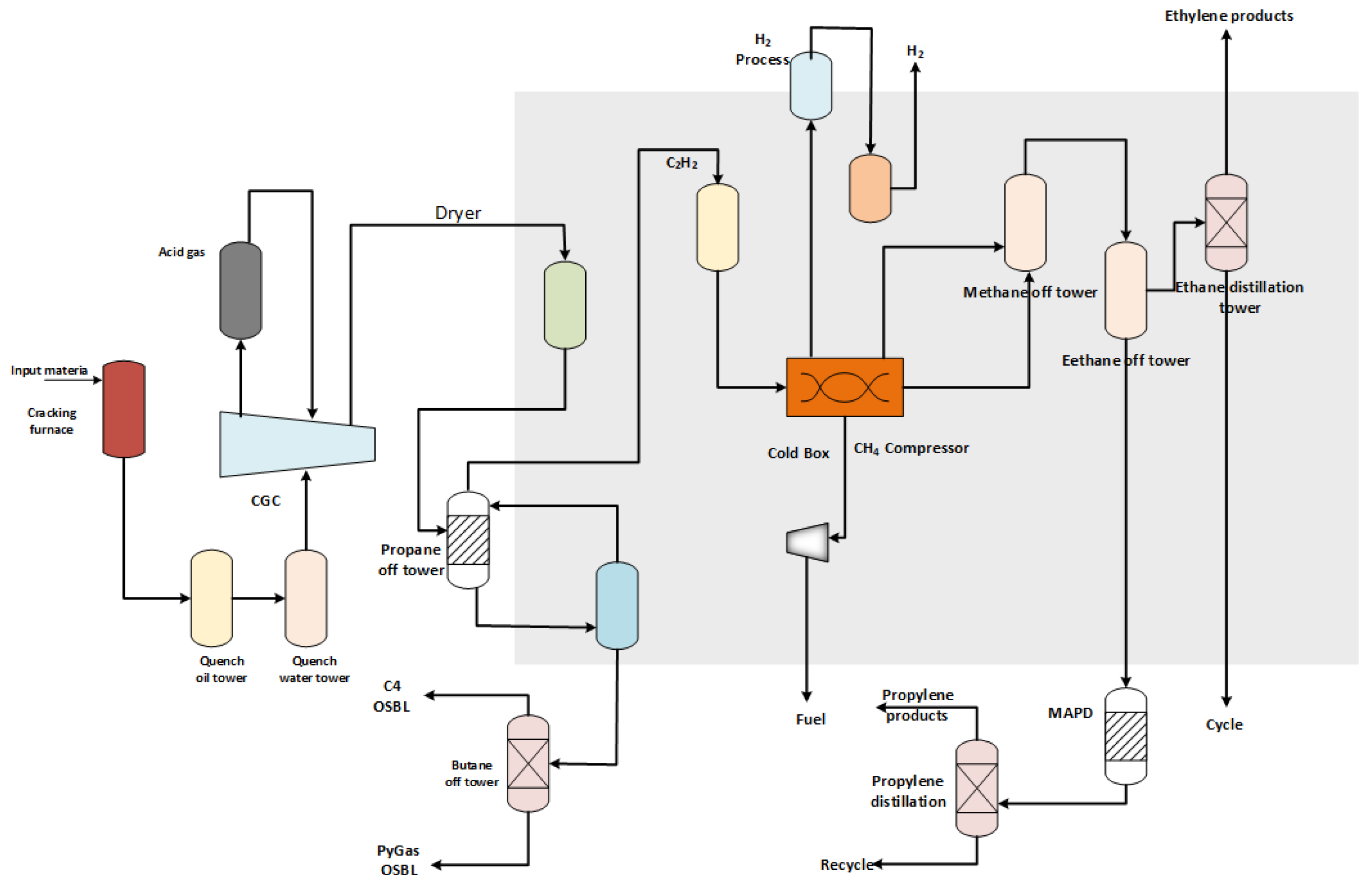
4.1. Ethylene Production Process

Ethylene production consists of cracking of the feedstock and separation of the product. First, the feedstock is heated and cracked in a cracking furnace to produce cracked gas. The cracked gas is then rapidly cooled in a rapid cooling tower to recover heat and undergo initial separation. This process requires large amounts of fuel, feedstock, and water. Afterwards, the cracked gas compressor (CGC) compresses the cracked gas to a high pressure, consuming electricity. The compressed gas is then dried before entering the deep-cooled separation unit. In this unit, components such as ethane and methane are separated through a cold box and a multi-stage separation tower. High-purity products such as ethylene and propylene are extracted. By-products like butane and cracked gasoline are processed separately. Throughout the ethylene production process, the output of ethylene is closely tied to basic resources such as fuel, crude oil, steam, electricity, and water. By optimizing the input ratios of these raw materials, production efficiency can be improved. This also helps achieve energy savings and emission reductions in the ethylene industry. The production process flow of the ethylene plant is shown in Figure 6.

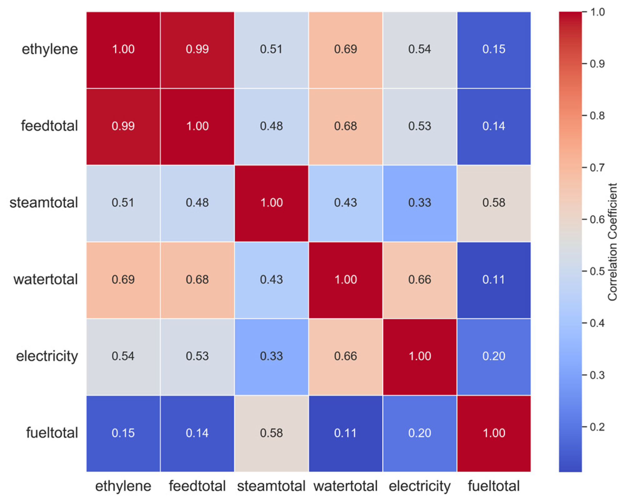
4.2. Analysis of the Ethylene Production Data

The dataset used in this paper contains the ethylene industrial production data from several chemical plants in China collected from 2009–2018. The input data consist of five relevant variables related to ethylene production as input data to construct the ethylene prediction model.

Table 1. Variables used in model construction.

Type	Variables	Unit
Input	Watertotal	ton
	Steamtotal	ton
	Fueltotal	ton
	Feedtotal	ton
	Electricity	kWh/ton
Output	Ethylene	ton/y

demonstrates the relevant variable names.

As shown in Figure 7, the three variables in the graph, steamtotal, fueltotal, and ethylene, are overall positively correlated. However, steamtotal and ethylene show negative correlation in time (1) and positive correlation in time (2). This reflects the complex interactions for different variables in the ethylene production process. Therefore, in order to extract the multivariate characteristics of the ethylene production process, the MPPT is proposed to construct the interaction relationship between different variables.

In a continuous time-varying data way, the data contain both local fluctuation changes and the overall trend of the data. To demonstrate the necessity of multigranularity modeling, we conducted comparative experiments on the relationships between variables at different granularities. First, we calculated the sample entropy of the same input and output variables at different granularities, as shown in

Table 2. Sample entropy at different granularities.

	Fueltotal (ton)	Electricity (kWh/ton)	Watertotal (ton)	Steamtotal (ton)	Feedtotal (ton)	Ethylene (ton/y)
Granularity 1	1.522	2.007	1.895	1.704	1.343	1.39
Granularity 2	1.819	2.397	2.621	1.927	2.397	2.061

. From the table, it can be observed that the sample entropy of each input and output variable differs across the two granularities. The sample entropy of the same variable varies across different granularities. A larger sample entropy indicates a more complex signal with more information content. This complexity refers to the diversity and unpredictability exhibited by the signal at different granularities. When the sample entropy increases, the data are more expressive of the general trend and less expressive of local fluctuation changes. With granularity 1, it is easier to observe the small local fluctuations in the data due to the larger sampling frequency of the data. With granularity 2, the change in the overall trend of the data becomes more significant because the sampling frequency of the data decreases. Therefore, integrating data from different time granularities can reveal short-term characteristics and detailed information. It also captures long-term trends and low-frequency changes, aiding in the analysis and understanding of the dynamic characteristics and complexity of the data.

To further demonstrate the importance of multigranularity modeling, we also calculated the feature correlations at granularity 1 and granularity 2 using the Pearson correlation coefficient. The correlation heatmaps are shown in Figure 8 and Figure 9. A higher correlation between two variables indicates a stronger association between them. As can be seen in Figure 8 and Figure 9, the input and output variables exhibit overall correlations. However, the degree of correlation between variables varies across different granularities. Under granularity 1, the correlation between ethylene and feedtotal and watertotal is more significant, reaching 0.99 and 0.78, respectively. In granularity 2, the correlation between ethylene and feedtotal and steamtotal is more significant, reaching 0.77 and 0.69, respectively. This indicates that the correlations between variables change at different time granularities, and modeling only single-granularity data may overlook some important features. Therefore, integrating data from multiple time granularities can help to reveal the diversity of data and the complex relationships between variables at different granularities. Overall, the comparative experiments on sample entropy and correlation at the two time- granularities fully demonstrate the necessity of multigranularity modeling. Modeling multigranularity data not only enables the extraction of interaction features between different input variables but also captures a more comprehensive feature representation between the inputs and outputs. Moreover, modeling multigranularity data and integrating correlation changes at different time granularities can enhance the model’s robustness. This improves both the accuracy and adaptability of predictions.

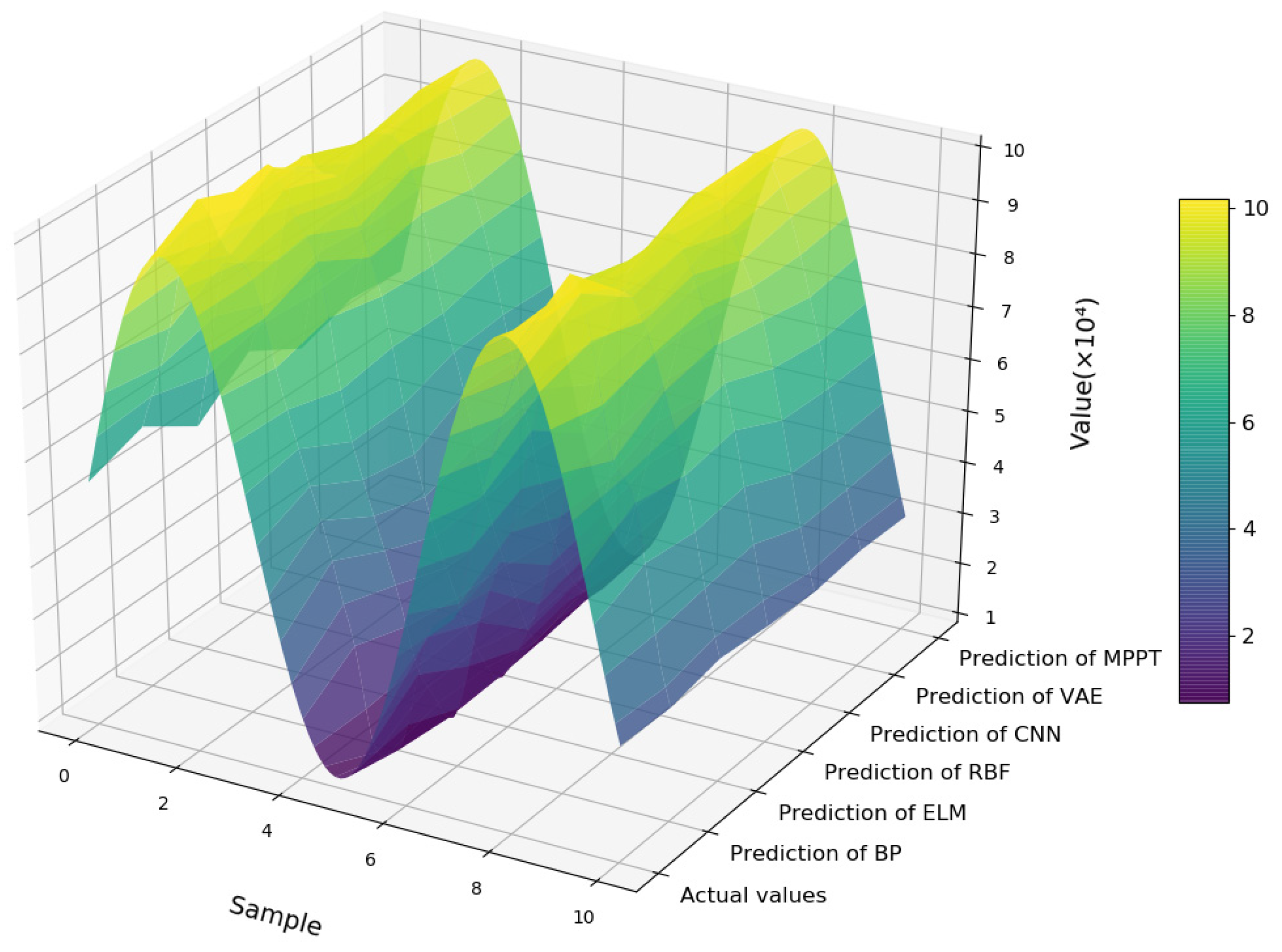
4.3. Case Analysis: Production Prediction and Energy Conservation of Ethylene Production Process

In order to verify the validity and reliability of MPPT, we used ethylene production as the output. The ethylene dataset was divided into a training set, a test set, and a validation set in the ratio of 8:1:1. The training set, validation set, and test set are used to train the model, tune the model parameters, and evaluate the predictive performance of the model, respectively. The model experiments were performed using Adam optimizer with learning rate set to 3 × 10⁻⁴ and batch size set to 32. The results of each model on the test set are shown in

Table 3. Experimental result of ethylene prediction.

Methods	MAE	RMSE
BP [11]	0.0394	0.508
ELM [14]	0.0375	0.4572
RBF [17]	0.0346	0.3906
CNN [20]	0.0286	0.328
VAE [29]	0.013	0.1935
MPPT	0.006	0.1755

. The prediction results of MPPT with other models are shown in Figure 10. It can be observed that the curve of the MPPT prediction results is the most similar to the actual values. To further clearly demonstrate the accuracy of the MPPT predictions, we compared the MPPT prediction results with the actual values, as shown in Figure 11.

Compared with traditional shallow neural networks like BP, ELM, and RBF, the MAE and RMSE of deep learning methods such as CNN and VAE are significantly reduced. Specifically, compared to RBF, CNN achieves a 17.3% reduction in MAE and a 16% reduction in RMSE. This demonstrates that deep learning methods have superior feature extraction and modeling capabilities, especially in complex chemical environments like ethylene production. Meanwhile, the MAE and RMSE of VAE decreased by 54.5% and 41%, respectively, compared with that of CNN. This indicates that the feature extraction ability of the model can be further enhanced by using KL dispersion to map the data distribution to the potential space. Comparing MPPT with VAE, the MAE and RMSE of MPPT decreased by 53.8% and 9.3%, which proved the effectiveness of multigranularity feature extraction.

The series of experiments above demonstrate the effectiveness of the MPPT model in ethylene yield prediction, achieving a prediction accuracy of 97%. Compared to other models that rely solely on single-granularity data, the MPPT model achieves lower MAE and RMSE. This proves that multigranularity modeling can more effectively extract multivariable interaction features, as well as the dynamic temporal relationships and nonlinear mapping between inputs and outputs in complex chemical production data.

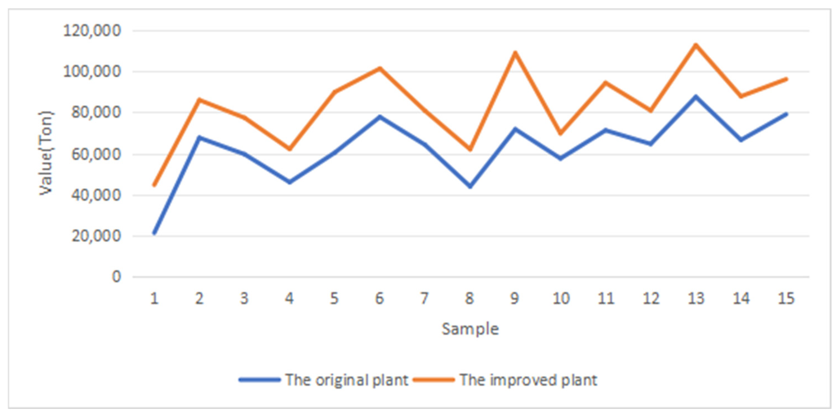
4.4. Energy Efficiency Optimization

Based on the prediction accuracy of the MPPT model, the ethylene yield can be predicted according to the input proportions of raw materials in the ethylene production process. Specifically, the initial configuration of raw material inputs is determined using historical data, followed by adjustments to the input proportions and subsequent predictions of ethylene yield to identify the optimal input ratio. The optimization strategy involves the following approaches: identifying raw materials that are excessively consumed but have a limited impact on improving ethylene yield, such as steam and water; increasing key raw materials that have a significant impact on ethylene yield, such as feedtotal. Overall, the optimization strategy operates at a system level. Instead of focusing solely on single variables, it adopts a holistic approach that considers the dynamic relationships among all raw materials and adjusts the input structure of the entire production process. The production input ratio can be adjusted to find the optimal raw material proportion based on predicting the ethylene production under different production inputs, as shown in Figure 12.

Using the eighth sample point in Figure 12 as an example, the comparison of production inputs before and after optimization of the ethylene production unit is shown in Figure 13. Compared with the original material consumption, the material consumption of the ethylene production unit after optimization, fueltotal, steamtotal, watertotal, and electricity decreased by 0.43 × 10⁴ tons, 5.38 tons, 1.386 tons, and 0.059 kWh/ton, respectively. Feedtotal increased by 1.9823 tons. After the production input optimization, the ethylene production increased by 2.1134 × 10⁴ tons. Using the MPPT model, we predicted ethylene production under different plant inputs. The MPPT can achieve energy savings, and reduced emissions, which demonstrated superiority of MPPT in energy efficiency optimization. Meanwhile, the improved plant will reduce CO₂ emissions by 5833 tons.

5. Discussion

5.1. Limitation Discussion

To evaluate the impact of the hyperparameter k, which determines the number of high-amplitude frequencies retained in the multiscale decomposition (MSD) module, we conducted a series of comparative experiments. The choice of k directly affects the granularity of the time-series data and, consequently, the model’s ability to capture multiscale features.

To select the optimal hyperparameter k, we conducted comparative experiments with different values of k = {1,2,4,8,16}, and determined the best hyperparameter based on evaluation metrics such as MAE, RMSE, and training time. For each value of k, the model was trained and evaluated on the same training, validation, and test datasets using consistent settings, including a learning rate of 3 × 10⁻⁴, a batch size of 32, and the Adam optimizer. The results of the comparison test are shown in Figure 14 and Figure 15.

The experimental results show that the training time increases with the increase in k. However, for MAE and RMSE, the results are no longer proportional to the changes in k. By considering the training time, MAE, and RMSE together, it can be observed that the model achieves the best performance when k = 4.

5.2. Results and Discussion

In the experimental section, we focused on the necessity, effectiveness, and application of multigranularity modeling, concluding with energy efficiency optimization using the MPPT model. To demonstrate the necessity of multigranularity modeling, two comparative experiments were conducted: sample entropy comparison and correlation analysis at different granularities. The sample entropy comparison revealed that the complexity and informational content of data vary across granularities. Multigranularity modeling facilitates the simultaneous capture of short-term characteristics and long-term trends, thereby enabling a better understanding of the dynamic properties and complexity of the data. In the correlation analysis, we observed that the degree of correlation between variables changes across granularities. This indicates that single-granularity modeling may overlook critical features, while multigranularity integration uncovers the diversity and intricate relationships within the data, enhancing model robustness and predictive capabilities.

Subsequently, we employed the MPPT model for multigranularity data modeling and compared its performance with other models. The experimental results showed that the MPPT model achieved the best performance, demonstrating its superior capability in extracting dynamic features and improving prediction accuracy and adaptability. Finally, we applied the MPPT model to optimize the ethylene production structure, resulting in increased ethylene yield and achieving energy savings and emission reduction. However, there are still some potential challenges in deploying the MPPT model in industrial environments. Due to the computational complexity of the MPPT model and the real-time requirements of practical applications, it imposes certain performance demands on GPUs or TPUs. Additionally, since the data distribution and variable characteristics may vary across different industrial scenarios, the MPPT model needs to be retrained or fine-tuned, making its adaptability to new industrial environments a significant challenge. Addressing these challenges will be the focus of our future research.

6. Conclusions

This paper proposes a novel MPPT model, which extracts interaction features of time series at different granularities, enabling the accurate prediction of complex chemical process data. The MPPT consists of MSD, PPT, and MF models. The MSD module transforms the industrial process data into multigranularity input data. Then, the PPT extracts the dynamic multigranularity data interaction features. The sample entropy and correlation of the input data variables were analyzed, which showed that the input variables exhibit different correlations at different granularities. Comparing MPPT with VAE, the MAE and RMSE of MPPT decreased by 53.8% and 9.3%, respectively, demonstrating the superior effectiveness of multigranularity feature extraction in improving prediction accuracy. Utilizing the accurate predictions of ethylene production provided by MPPT, the production input ratio was optimized to determine the optimal raw material proportions. As a result, the material consumption of the ethylene production unit was significantly reduced: fueltotal decreased by 0.43 × 10⁴ tons, steamtotal by 5.38 tons, watertotal by 1.386 tons, and electricity by 0.059 kWh/ton. These reductions highlight the MPPT model’s capability to enhance energy efficiency and achieve substantial resource savings in industrial applications. The MPPT can achieve energy savings, and reduced emissions, which demonstrated superiority of MPPT in energy efficiency optimization.

In the future, we will integrate large language models (LLMs) to guide production optimization scheduling. Combining LLMs and MPPT for optimizing the ethylene production structure holds great potential. LLMs can process and analyze vast amounts of structured and unstructured data, providing valuable optimization insights. Leveraging LLMs for optimization scheduling helps identify inefficiencies, propose improvement measures, and perform predictive analyses based on historical or real-time data. This integration facilitates intelligent production structure optimization, enabling autonomous adjustment of input proportions during continuous production, thereby promoting sustainable development in the petrochemical industry.

References

1. Tian, C.; Liang, Y.; Lin, Q.; You, D.; Liu, Z. Environmental Pressure Exerted by the Petrochemical Industry and Urban Environmental Resilience: Evidence from Chinese Petrochemical Port Cities. J. Clean. Prod. 2024, 471, 143430. [Google Scholar] [CrossRef]
2. Chen, Q.; Lv, M.; Wang, D.; Tang, Z.; Wei, W.; Sun, Y. Eco-Efficiency Assessment for Global Warming Potential of Ethylene Production Processes: A Case Study of China. J. Clean. Prod. 2017, 142, 3109–3116. [Google Scholar] [CrossRef]
3. Geng, Z.; Zhang, Y.; Li, C.; Han, Y.; Cui, Y.; Yu, B. Energy Optimization and Prediction Modeling of Petrochemical Industries: An Improved Convolutional Neural Network Based on Cross-Feature. Energy 2020, 194, 116851. [Google Scholar] [CrossRef]
4. Li, Q.; Zhang, M.; Shi, X.; Lan, X.; Guo, X.; Guan, Y. An Intelligent Hybrid Feature Subset Selection and Production Pattern Recognition Method for Modeling Ethylene Plant. J. Anal. Appl. Pyrolysis 2021, 160, 105352. [Google Scholar] [CrossRef]
5. Wang, Y.; Tang, B.; Tao, W.; Yuan, A.; Li, T.; Liu, Z.; Zhang, F.; Mao, A. Triaxial Compression Strength Prediction of Fissured Rocks in Deep-Buried Coal Mines Based on an Improved Back Propagation Neural Network Model. Processes 2023, 11, 2414. [Google Scholar] [CrossRef]
6. Wang, R.; Chen, L.; Huang, Z.; Zhang, W.; Wu, S. A Review on the High-Efficiency Detection and Precision Positioning Technology Application of Agricultural Robots. Processes 2024, 12, 1833. [Google Scholar] [CrossRef]
7. Zhang, R.; Wang, Y.; Wang, K.; Zhao, H.; Xu, S.; Mu, L.; Zhou, G. An Evaluating Model for Smart Growth Plan Based on BP Neural Network and Set Pair Analysis. J. Clean. Prod. 2019, 226, 928–939. [Google Scholar] [CrossRef]
8. Zhang, M.; Cao, D.; Lan, X.; Shi, X.; Gao, J. An Ensemble-Learning Approach To Predict the Coke Yield of Commercial FCC Unit. Ind. Eng. Chem. Res. 2022, 61, 8422–8431. [Google Scholar] [CrossRef]
9. Singh, B. MOWM: Multiple Overlapping Window Method for RBF Based Missing Value Prediction on Big Data. Expert Syst. Appl. 2019, 122, 303–318. [Google Scholar] [CrossRef]
10. Wei, L.; Yumin, S. Prediction of Energy Production and Energy Consumption Based on BP Neural Networks. In Proceedings of the 2008 IEEE International Symposium on Knowledge Acquisition and Modeling Workshop, Wuhan, China, 21–22 December 2008; pp. 176–179. [Google Scholar]
11. Liang, W.; Wang, G.; Ning, X.; Zhang, J.; Li, Y.; Jiang, C.; Zhang, N. Application of BP Neural Network to the Prediction of Coal Ash Melting Characteristic Temperature. Fuel 2020, 260, 116324. [Google Scholar] [CrossRef]
12. Yu, F.; Xu, X. A Short-Term Load Forecasting Model of Natural Gas Based on Optimized Genetic Algorithm and Improved BP Neural Network. Appl. Energy 2014, 134, 102–113. [Google Scholar] [CrossRef]
13. Han, Y.; Wu, H.; Jia, M.; Geng, Z.; Zhong, Y. Production Capacity Analysis and Energy Optimization of Complex Petrochemical Industries Using Novel Extreme Learning Machine Integrating Affinity Propagation. Energy Convers. Manag. 2019, 180, 240–249. [Google Scholar] [CrossRef]
14. Ji, Y.; Zhang, S.; Yin, Y.; Su, X. Application of the Improved the ELM Algorithm for Prediction of Blast Furnace Gas Utilization Rate. IFAC-Pap. 2018, 51, 59–64. [Google Scholar] [CrossRef]
15. Geng, Z.; Qin, L.; Han, Y.; Zhu, Q. Energy Saving and Prediction Modeling of Petrochemical Industries: A Novel ELM Based on FAHP. Energy 2017, 122, 350–362. [Google Scholar] [CrossRef]
16. Zhu, Q.-X.; Zhang, X.-H.; Wang, Y.; Xu, Y.; He, Y.-L. A Novel Intelligent Model Integrating PLSR with RBF-Kernel Based Extreme Learning Machine: Application to Modelling Petrochemical Process. IFAC-Pap. 2019, 52, 148–153. [Google Scholar] [CrossRef]
17. Han, H.-G.; Chen, Q.; Qiao, J.-F. An Efficient Self-Organizing RBF Neural Network for Water Quality Prediction. Neural Netw. 2011, 24, 717–725. [Google Scholar] [CrossRef]
18. Aghbashlo, M.; Hosseinpour, S.; Tabatabaei, M.; Dadak, A.; Younesi, H.; Najafpour, G. Multi-Objective Exergetic Optimization of Continuous Photo-Biohydrogen Production Process Using a Novel Hybrid Fuzzy Clustering-Ranking Approach Coupled with Radial Basis Function (RBF) Neural Network. Int. J. Hydrogen Energy 2016, 41, 18418–18430. [Google Scholar] [CrossRef]
19. Li, J.; Zhang, R.; Wang, H.; Xu, Z. Inverse Problem of Permeability Field under Multi-Well Conditions Using TgCNN-Based Surrogate Model. Processes 2024, 12, 1934. [Google Scholar] [CrossRef]
20. Yuan, X.; Qi, S.; Wang, Y.; Xia, H. A Dynamic CNN for Nonlinear Dynamic Feature Learning in Soft Sensor Modeling of Industrial Process Data. Control. Eng. Pract. 2020, 104, 104614. [Google Scholar] [CrossRef]
21. Shi, X.; Huang, G.; Hao, X.; Yang, Y.; Li, Z. Sliding Window and Dual-Channel CNN (SWDC-CNN): A Novel Method for Synchronous Prediction of Coal and Electricity Consumption in Cement Calcination Process. Appl. Soft Comput. 2022, 129, 109520. [Google Scholar] [CrossRef]
22. Han, Y.; Wang, Y.; Chen, Z.; Lu, Y.; Hu, X.; Chen, L.; Geng, Z. Multiscale Variational Autoencoder Regressor for Production Prediction and Energy Saving of Industrial Processes. Chem. Eng. Sci. 2024, 284, 119529. [Google Scholar] [CrossRef]
23. Jang, K.; Hong, S.; Kim, M.; Na, J.; Moon, I. Adversarial Autoencoder Based Feature Learning for Fault Detection in Industrial Processes. IEEE Trans. Ind. Inform. 2021, 18, 827–834. [Google Scholar] [CrossRef]
24. Laubscher, R.; Rousseau, P. Application of Generative Deep Learning to Predict Temperature, Flow and Species Distributions Using Simulation Data of a Methane Combustor. Int. J. Heat Mass Transf. 2020, 163, 120417. [Google Scholar] [CrossRef]
25. Vaswani, A.; Shazeer, N.; Parmar, N.; Uszkoreit, J.; Jones, L.; Gomez, A.N.; Kaiser, L.; Polosukhin, I. Attention Is All You Need. In Proceedings of the Annual Conference on Neural Information Processing Systems 2017, Long Beach, CA, USA, 4–9 December 2017; pp. 6000–6010. [Google Scholar]
26. Liu, D.; Wang, Y.; Liu, C.; Yuan, X.; Yang, C.; Gui, W. Data Mode Related Interpretable Transformer Network for Predictive Modeling and Key Sample Analysis in Industrial Processes. IEEE Trans. Ind. Inform. 2022, 19, 9325–9336. [Google Scholar] [CrossRef]
27. Han, Y.; Han, L.; Shi, X.; Li, J.; Huang, X.; Hu, X.; Chu, C.; Geng, Z. Novel CNN-Based Transformer Integrating Boruta Algorithm for Production Prediction Modeling and Energy Saving of Industrial Processes. Expert Syst. Appl. 2024, 255, 124447. [Google Scholar] [CrossRef]
28. Liu, D.; Wang, Y.; Yuan, X.; Yang, C. Multirate-Former: An Efficient Transformer-Based Hierarchical Network for Multistep Prediction of Multirate Industrial Processes. IEEE Trans. Instrum. Meas. 2024, 73, 1–13. [Google Scholar] [CrossRef]
29. Lee, Y.S.; Chen, J. Developing Semi-Supervised Latent Dynamic Variational Autoencoders to Enhance Prediction Performance of Product Quality. Chem. Eng. Sci. 2023, 265, 118192. [Google Scholar] [CrossRef]
Figure 1. An overview of MSD. Industrial process data are transformed into spectral data through Fast Fourier Transform (FFT), with the top-K frequencies having the highest amplitudes selected to reconstruct K inputs at different granularities.
Processes 13 00104 g001
Figure 2. Structure of parallel pyramidal Transformer module. The PCM module uses multiple convolution operations to construct the input data into a pyramid structure, generating multilayer sequences from coarse to fine granularity. The PIM module connects adjacent nodes at the same scale and parent–child nodes across different scales to capture the long-term and short-term dependencies of the time series.
Processes 13 00104 g002
Figure 3. Structure of pyramid construction module. The input data are first dimensionally reduced through a linear layer, then processed through multiple convolutional layers to obtain sequences at different scales, and finally, the sequences at different scales are concatenated to form a pyramid structure.
Processes 13 00104 g003
Figure 4. Structure of pyramid interaction module. The PIM consists of two parts: Intra-Scale connections and Inter-Scale connections. Inter-Scale connections construct a multi-resolution representation of the sequence and Intra-Scale connections capture temporal dependencies at different resolutions by connecting consecutive neighboring nodes.
Processes 13 00104 g004
Figure 5. An overview of multigranularity parallel pyramidal Transformer which consists of MSD, PPT, and FM.
Processes 13 00104 g005
Figure 6. The production process of the ethylene plant.
Processes 13 00104 g006
Figure 7. The ethylene production industry analysis.
Processes 13 00104 g007
Figure 8. Calculation of feature correlation at granularity 1.
Processes 13 00104 g008
Figure 9. Calculation of feature correlation at granularity 2.
Processes 13 00104 g009
Figure 10. The comparison of prediction results.
Processes 13 00104 g010
Figure 11. The prediction results of the MPPT.
Processes 13 00104 g011
Figure 12. Comparison of production capacity of ethylene production plants.
Processes 13 00104 g012
Figure 13. Comparison of total material consumption in ethylene production plants.
Processes 13 00104 g013
Figure 14. Comparison of training time with different hyperparameters k.
Processes 13 00104 g014
Figure 15. Comparison of MAE and RMSE with different hyperparameters k.
Processes 13 00104 g015