Potato Beetle Detection with Real-Time and Deep Learning

Abstract

In this study, deep learning methods were used to detect potato beetles (Leptinotarsa decemlineata) on potato plants. High-resolution images were taken of fields with the help of a drone. Since these images were large in size, each one was divided into six equal parts. Then, according to the image, the potato beetles were divided into three classes: adult, late-stage potato beetle, and no beetles. A data set was created with 3000 images in each class, making 9000 in total. Different filters were applied to the images that made up the data set. In this way, problems that may have arisen from the camera in real-time detection were minimized. At the same time, the accuracy rate was increased. The created data set was used with six different deep learning models: MobileNet, InceptionV3, ResNet101, AlexNet, DenseNet121, and Xception. The deep learning models were tested with Sgd, Adam, and Rmsprop optimization methods and their performances were compared. In order to evaluate the success of the models more accurately, they were tested on a second data set created with images taken from a different field. As a result of this study, the highest accuracy of 99.81% was obtained. In the test results from a second field that did not exist in the data set, 92.95% accuracy was obtained. The average accuracy rate was 96.30%.

1. Introduction

Potatoes are preferred to be grown due to their features such as their high yield per unit area, high nutritional value, and ease of adaptation to different climatic regions. In addition, potatoes are an annual crop plant that can easily grow in many parts of the world and are used as an important food source. Potatoes are a very valuable food source and their consumption is increasing day by day. With their high nutritional value and wide range of uses, they are one of the most important foods and could be a solution to the growing world hunger problem [1].

Potato farming occurs in the majority of countries in the world. Potatoes are ranked after wheat, corn, and rice in terms of production amount. There are many diseases and pests that cause yield loss in potato plants. The potato beetle is the most critically important among these [2].

Monitoring plant health, the early detection of diseases and pests, and taking necessary precautions in a timely manner minimize losses in plant production. At the same time, it is of great importance to increase the amount of product taken from the unit area and to improve the product quality [3]. Machine learning algorithms, computer vision, and hardware developments are promising in terms of finding solutions to problems in agriculture [4]. With the development of modern computer science, computer vision has become an increasingly widely used approach to categorize pests because traditional pest classification methods have high time and labor requirements [5]. There are many different studies on this topic in the literature. A study was conducted using artificial neural networks to automatically classify Mexican bean beetle and Colorado potato beetle adults, which are leaf pests of potato and bean plants. It was found that the RSC classifier provided a recognition rate of 89% and the LIRA classifier provided a recognition rate of 88%. It has been claimed that these results are sufficient for pest detection and can be used to identify locations that may be harmful to plants [6]. Liu et al. proposed a classifier called PestNet for deep-learning-based large-scale multi-class pest detection and classification. They found the average mAP value of PestNet for all classes to be 75.46% [7]. The early and accurate classification of pests that cause major problems in the agricultural sector reduces economic losses and helps with the measures to be taken. It has been demonstrated that recent developments in deep learning convolutional neural networks have greatly increased the accuracy of image recognition systems [8].

In their study, Cheeti emphasized that the YOLO algorithm could be used for pest detection and the convolutional neural network algorithm for classification and that the detection and classification of pests is important in the fight against them [9]. In their study, Chan and colleagues detected insects from images of sticky traps with the YOLOv4 deep learning algorithm. They stated that the type of insect was determined from this image with the GoogLeNet Inceptionv4 algorithm. As a result of their study, they calculated the accuracy rate of the object detection model as 96% and the accuracy rate of the species identification model as 87.1% [10]. Wang and his colleagues developed an automatic system for monitoring pests in large agricultural areas, instead of manual prediction methods. Thanks to this system, information about the type and number of pests was obtained. The time and cost of integrated pest control in these studies have been greatly reduced. This therefore suggests that the excessive use of pesticides can be prevented [11].

Many plants are being studied for the early detection of diseases. Different artificial intelligence methods are used in these studies. In one study, a data set consisting of 380 photographs was prepared to detect jute pests. This data set was used with different deep learning algorithms. The highest accuracy rate was 99%, which was with the DenseNet201 architecture [12]. There are different studies on disease detection in banana plants. Their common feature is disease detection using leaves. Disease detection is achieved by examining the leaves of banana plants. Five different architectures were used in the deep learning algorithm for this. The highest rate was 96.25%, which was found with the BananaSqueezeNet model [13]. In another study focusing on machine learning, a data set consisting of 1600 banana leaves was used. The highest accuracy rate was 93.7% [14]. Another plant where diseases can be detected using leaves is mango. In a study, seven different disease detection methods were performed using mango leaves. Two different deep learning architectures were used in this study. The highest accuracy rate achieved was 98.55% [15]. Some diseases are caused by insects. To prevent them, the insects need to be detected before they grow. In the studies conducted related to this, the highest accuracy rate achieved was 90% [16,17,18,19].

The common theme in the literature is increasing the productivity of plants. This has been achieved using the detection of diseases and insects that cause low yield in plants. Ready-made data sets were used in these studies. In contrast, a new data set was created for potato beetle detection in this study. The created data set was used with six different deep learning architectures. Different filters were applied to the data set to increase the accuracy rates. In the real-time detection process, camera errors were transferred to the data set. To amend these, grayscale, noise addition, blurring, left and right rotation, brightness increase and decrease, cropping, horizontal rotation, and clockwise and counterclockwise rotation were applied to all the photos in the data set. In this study, the highest accuracy obtained was 99.81%. For the test results obtained from a second field that did not already exist in the data set, 92.95% accuracy was obtained. Average accuracy of 96.30% was obtained. In this study, a very easy, fast, and high-accuracy detection process was developed for real-time detection processes.

2. Materials and Methods

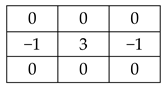
In this study, real-time detection of potato beetles on potato plants was carried out with a drone. For this purpose, firstly, a data set was prepared. This was a unique and new data set for the study. It was then run on six different deep learning architectures. Figure 1 shows the general working principle of the system.

2.1. Data Set

In this study, images were taken from two separate potato fields from different angles and heights with the help of a DJI Phantom 3 model drone. Of the first field, 5850 images were taken and 3150 images were taken of the second field. While the images taken of the first field were used for training and testing, the images taken of the second field were used only for testing purposes. Images collected on 43 different days, at different times of the day, at intervals of 2–3 days on average, were filed separately. The images taken of the fields have a high resolution of 2250 × 4000.

All images collected on different days and filed separately were combined in a single folder in the order of the day they were taken. Because all images were taken with the same camera, they are equal in size.

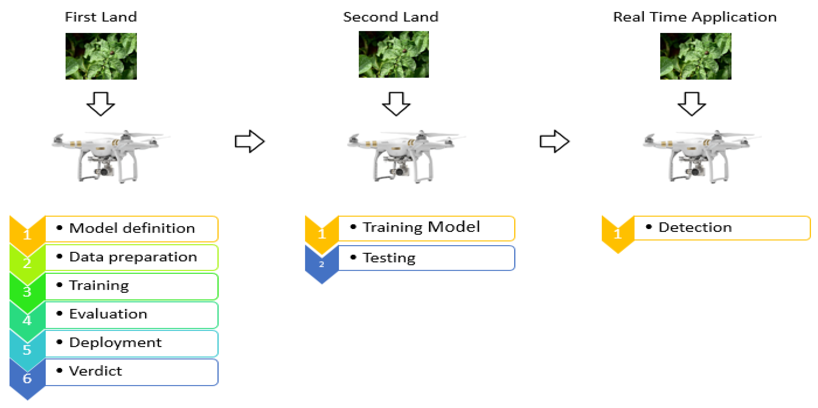
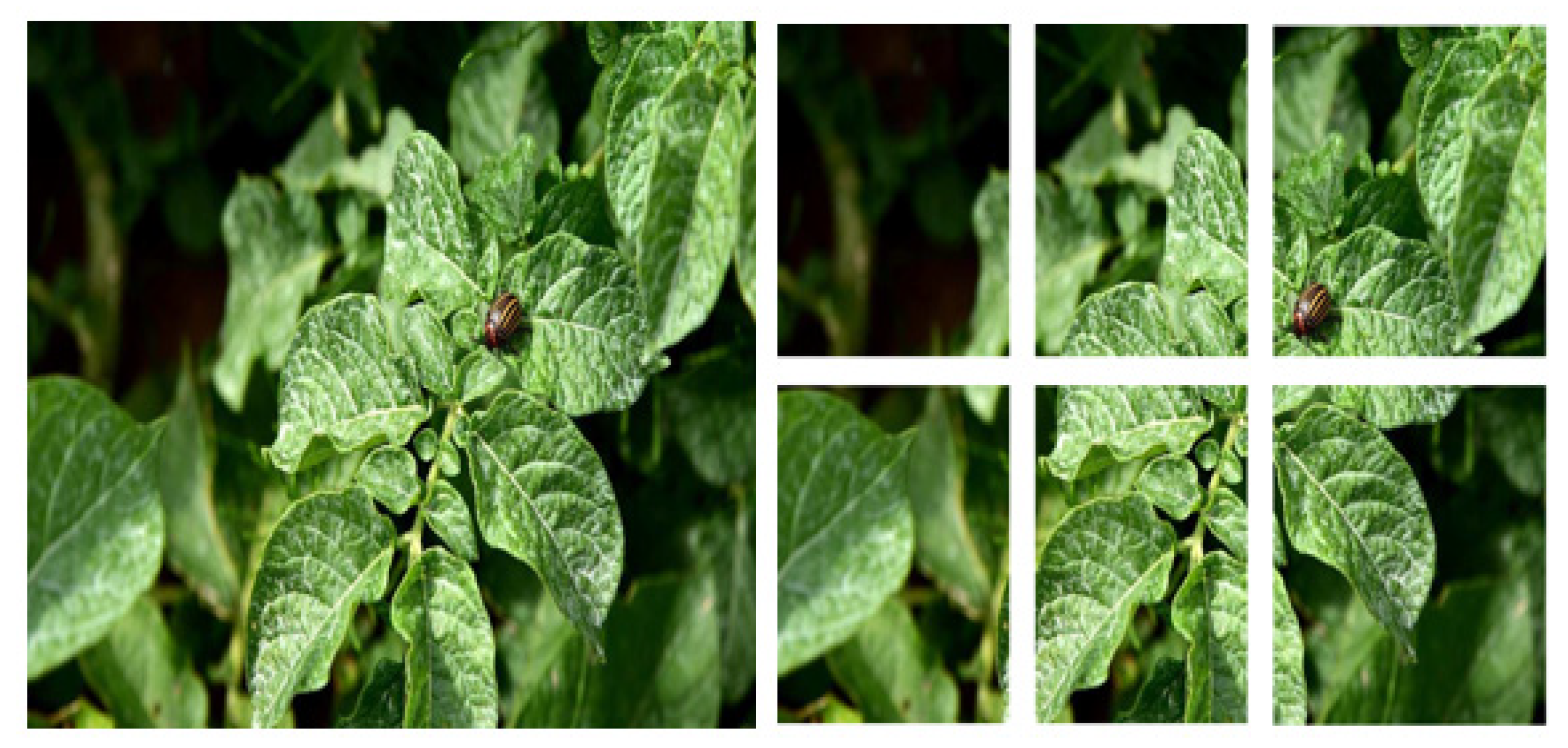
The original images are quite large and need to be reduced by approximately one-tenth during training to be suitable for the input of the network. In this case, it causes a lot of data loss. Additionally, the success of convolutional neural networks depends on the availability of large amounts of data. For this, the original images were divided into 6 equal parts. In this way, data loss was reduced. It also increased the data set size. In addition, split images also increase the diversity in the data set due to perspective differences. Figure 2 shows an example of an image divided into 6 equal parts.

Although the tested land had a smooth structure, differences occurred in some areas. On some plants, the potato beetles are in the adult state or in the final stage, while on some plants there are no insects. Therefore, not all parts of an original image are included in the same class. Each class in the data set was created from individually selected parts.

When all images were divided into 6 parts, a total of 37,820 images of the same pixel size were obtained. From these images, those that can be clearly distinguished by eye were selected and 3 separate classes were created and labeled.

Table 1. Description of each class of sunflower plant, number of samples, and number of samples after filtering.

Class Number	Class Description	Number of Images
1	It covers the first and second instars of the potato bugs. In these stages, the potato bugs are black. In the first stage, they feed on their shells. In the second phase, they disperse over the plant. They consume leaves irregularly from their edges.	17,925
2	In the third and fourth periods, the potato beetles spread further on the plant and cause significant damage by feeding on the leaf stems and trunk. At this stage, the front edge of the insect turns orange-brown.	12,700
3	There are no potato bugs.	7195

shows the definition and image numbers of each class.

Different filtering operations were performed on the data set used in the study. Thanks to these filters, the data set has been improved. At the same time, the data set size has been increased.

2.1.1. Blurring and Noise Removal

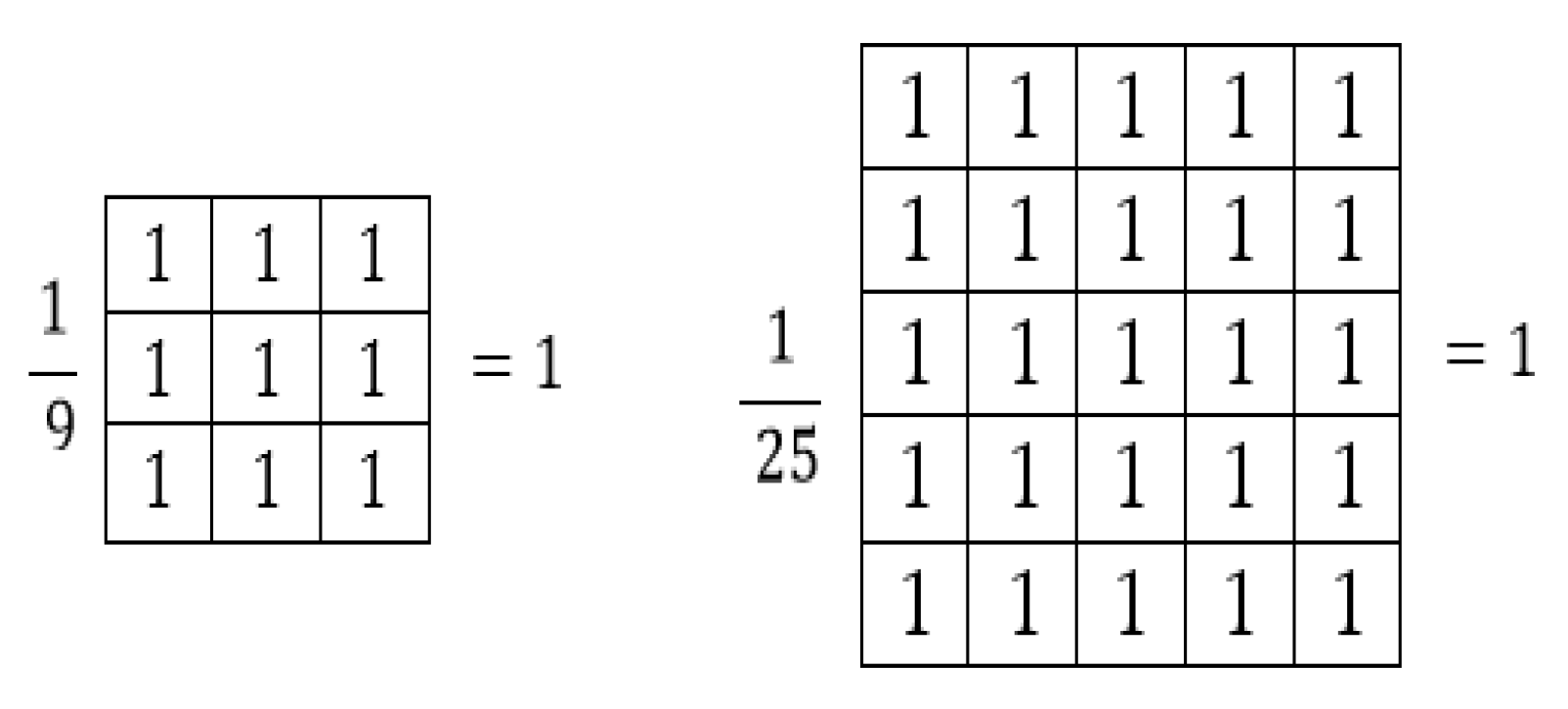
Blurring is a method of averaging the color of the pixels of the image within a certain area. With this method, the clarity of the picture is lost. In the filters used for this blurring, the coefficients must be positive. Average blur filters of 3 × 3 and 5 × 5 sizes are given as examples in Figure 3.

As can be seen from the filters, the sum of the coefficients is equal to 1. If the sum is greater or less than 1, the brightness of the image changes. Additionally, as the filter size increases, blurriness increases and details become less visible.

Other filters other than average blur are also available. The blurring process performed with the Gaussian function to reduce details and noise in the image is called Gaussian blurring. The method aims is to update the value of a pixel with the average of neighboring pixels. However, instead of the average of all neighboring pixels, the weighted average is calculated.

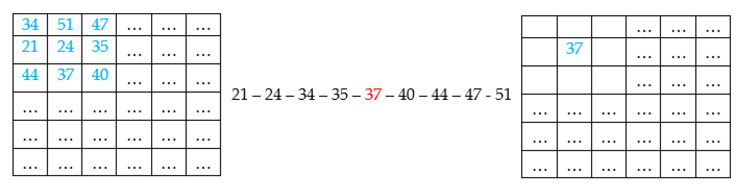
Noise can also be reduced with some statistical methods in image processing. The most well-known of these is the median filter. In the median filter, the values in the window range are sorted and the middle value is taken. Thus, excessive jumps are eliminated. The median filter is very successful in cleaning salt–pepper noise. Figure 4 shows the application of the median filter on images.

Other filters most commonly used to clean salt and pepper noise are maximum and minimum filters. In the maximum filter, the values within the window range are sorted and the largest value is taken, while in the minimum filter, the opposite is performed and the smallest value is taken. While the maximum filter is successful in cleaning pepper noise, the minimum filter is successful in cleaning salt noise.

2.1.2. Sharpening

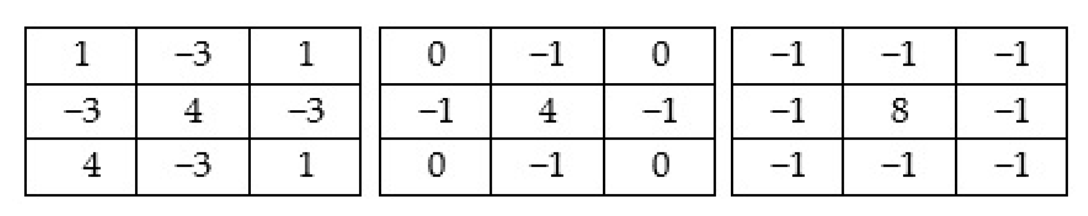
Unlike blurring, sharpening makes details more visible. Sharpening filters are mostly used for improving output quality, medical imaging, and industrial inspection. The filter matrices in Figure 5 can be used for sharpening purposes. As can be seen from the matrices, coefficients can be both negative and positive values. As the matrix size increases, the effect of the filter and also the processing time increase.

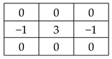
2.1.3. Edge Detection

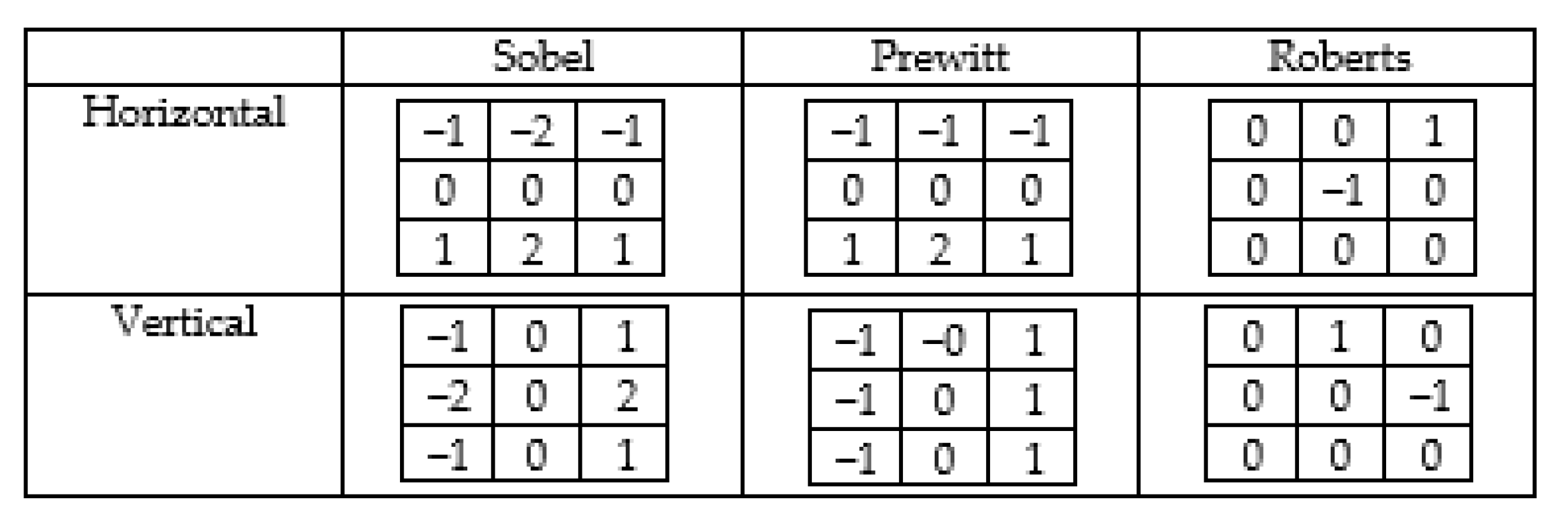
Edges are regions where there are sudden changes in the gray levels of an image. Edge information is one of the most needed features obtained from the image. It is often used to find the boundaries of objects, especially in object recognition applications. It symbolizes the high-frequency regions of the input information. To obtain edge information, convolution is applied separately with two filters, horizontally and vertically. There are many edge detection filters available in the literature. The most well-known are filters such as Sobel, Prewitt, Roberts, Laplace, and Canny.

Figure 6 shows the horizontal and vertical weight coefficients for Sobel, Prewitt, and Roberts edge detection filters. These filters capture sharpness in horizontal and vertical directions. This gives more weight to pixels on the axes. These masks can be used separately, or both can be used together. With the help of masks, the changing size of the middle pixel is calculated by taking into account the neighboring pixels.

2.1.4. Rotation

Images can be rotated horizontally or vertically or at certain angles around a certain center point according to the user’s wishes and needs. If the image is rotated to angles other than 90 and its multiples, overflows will occur in the output image. These overhangs can be cut off or filled with black or white.

2.1.5. Data Duplication

In the study, detection was carried out in real time. For this, images taken from the camera were used. For this, errors that may occur from the camera in real time must be introduced to the system. Otherwise, detection in real-time applications will occur with very low accuracy or the detection process will never occur. For this purpose, different processes were applied to the images that constitute the data set. 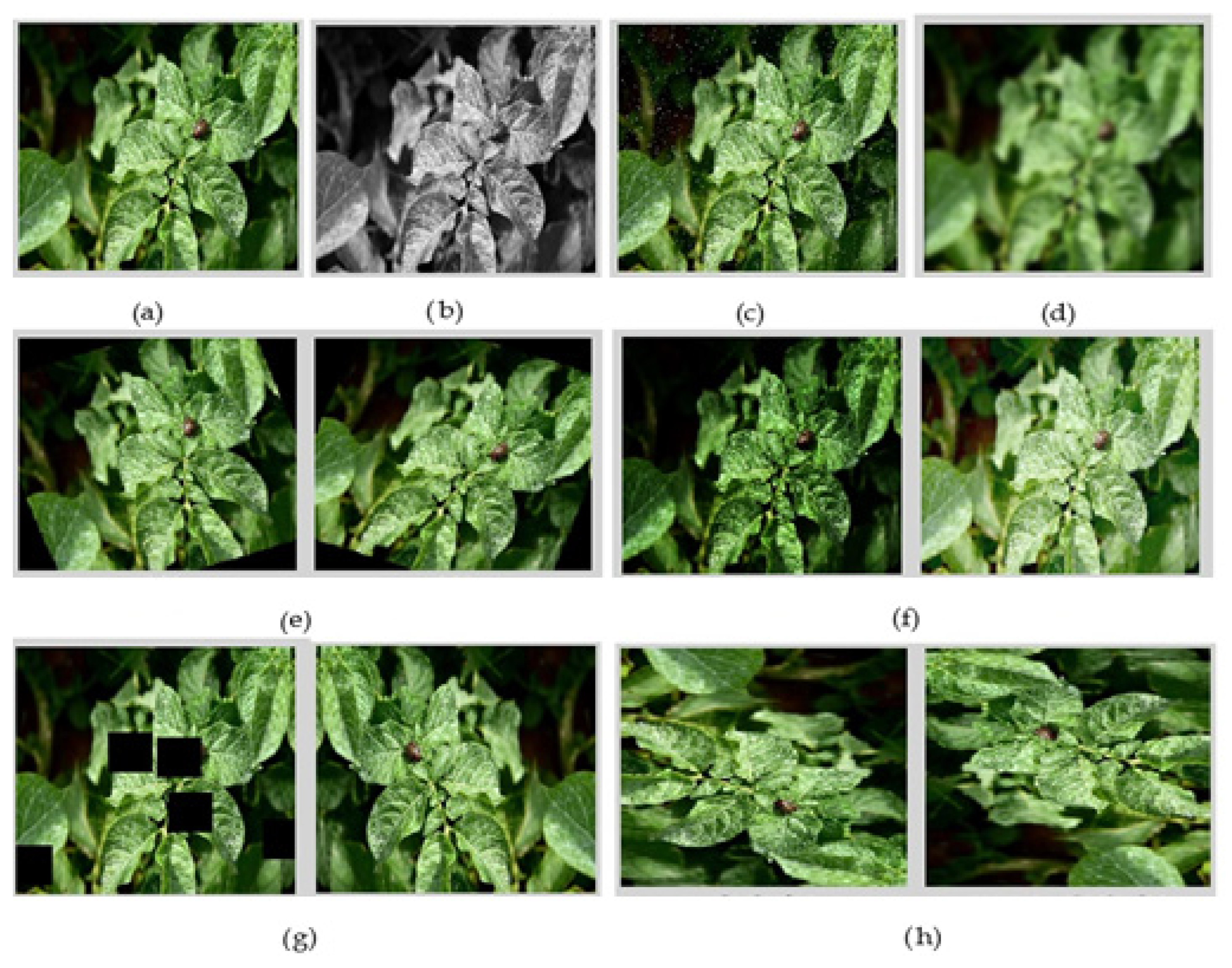Figure 7 shows the operations applied to the images that make up the data set.

Figure 7a shows the normal photo without modification. In Figure 7b, the images in the database have been converted to grayscale. In case of color loss that may occur in the camera, the system will continue to work. In Figure 7c, Gaussian blurring has been applied to the images in the database. Gaussian blur was performed randomly. In this way, the camera focus is ensured to be more resistant. In Figure 7d, noise has been added to increase robustness against camera artifacts. There are electronic devices for vehicles, especially mobile phones, which cause noise in the camera. To prevent this, noise was added to the images. In Figure 7e, +15% and −15% changes in image brightness were made to make the model robust to light and camera changes. The image taken with the camera is not always clear. Especially at sunset and sunrise, very clear photos cannot be taken. To prevent this, changes were made to the brightness of the images. In Figure 7f, +15% and −15% slopes were added to the images. The drone is mostly in motion, which means it vibrates and shakes. This causes shifts in the images. Therefore, +15% and −15% slopes were added to the images in the database, so the system can always detect the images. In Figure 7g, truncation has been added to help the model be more resistant to object occlusion. Some areas are not visible when taking photos with the camera. When an object moves in front of the camera, that part of the picture appears black. At such times, images were cropped to ensure that the detection process was working properly. In Figure 7h, the images are rotated clockwise and counterclockwise. These changes were made to minimize the impact of drone movement.

2.2. Deep Learning

Deep learning is a form of learning that imitates humans. In order to define a model in classical machine learning techniques, the feature vector must first be extracted by experts. Processing data with these techniques takes a long time and is only possible with the presence of an expert. Deep learning has eliminated this problem, which has been dealt with for many years, and performs learning with the help of deep multi-layer neural networks on raw data without the help of an expert or pre-processing.

Artificial neural network algorithms could not be used until the 2000s due to computational costs. In recent years, the operating speed of computers has increased. At the same time, with the use of GPU units in calculations, it has become possible to train deep networks without pre-training. Deep learning methods have attracted attention, especially after their success in a large-scale visual recognition competition held in 2012.

Since a large amount of data and many layers are used in deep learning methods, the learning process takes a very long time and may even last for days. Therefore, increasing the amount of data and the number of layers increases the learning time and requires more computing power for the hardware to be used. There are many different types of deep learning architectures built by increasing the number of layers. In some studies, hybrid models can be obtained by using these architectures together.

2.2.1. AlexNet

After the development of the LeNet model, no work was performed in this field for a long time. CNNs became popular again after the AlexNet model came first in the ILSVRC competition held in 2012. The structure of the AlexNet model, consisting of five convolutional and three fully connected layers, is given in detail in Figure 8.

In the AlexNet model, 96 filters with dimensions of 11 × 11 × 3 in the first convolution layer were convolved with 4-step intervals on the 224 × 224 × 3 images taken from the input layer. The second convolution layer takes the normalized and pooled outputs of the first convolution layer as input and applies convolution with 256 filters of size 5 × 5 × 48. The third convolution layer applies convolution with 384 filters of size 3 × 3 × 256 on the outputs of the second layer, where normalization and pooling are applied. The third, fourth, and fifth layers are connected without any normalization or pooling layers in between. In the fourth convolution layer, 384 filters of size 3 × 3 × 192 are used, and in the fifth convolution layer, 256 filters of size 3 × 3 × 192 are used. There are 4096 neurons in each fully connected layer. To prevent overfitting problems in the learning of the network, data augmentation and dilution processes were applied in the first two fully connected layers. In the last layer, classification is performed for 1000 different objects.

2.2.2. ResNet

It is the residual neural network (ResNet) model that won first place in the 2015 ILSVRC competition. It is designed to facilitate the training of models with much deeper structure than previously used models. Although it is thought that success will increase as the number of layers in a model increases, this is not the case. Due to vanishing or excessively increasing gradients (vanishing/exploding gradient), the training error increases instead of decreasing. As we go deeper into the flat structure, the learning process suffers losses and gradients become inoperable. However, in the ResNet structure, the network is not allowed to be affected by using old activation results. Figure 9 shows the skip connection used in the ResNet structure.

The ResNet model, whose main lines are inspired by the VGGNet model, has different versions with 18, 34, 50, 101, and 152 layers. The ResNet model consisting of 152 layers has 8 times more layers than the VGGNet model but has less complexity.

2.2.3. Xception

Xception was developed by Google, inspired by the Inception model. Xception is a convolutional neural network architecture consisting of deeply separable convolution steps instead of inception modules with residual connections. It has 36 convolutional layers that form the feature extraction base of the network. Even though it has the same number of parameters as InceptionV3, it performs significantly better. An open-source Xception application using Keras and TensorFlow is available as part of the Keras applications module.

2.2.4. MobileNet

Just like the Inception and Xception models, MobileNet was also designed by Google researchers. Developed for mobile and embedded vision applications, MobileNet uses deeply separable convolution blocks to reduce model size and complexity. These blocks consist of a deep convolution layer that filters the input and a 1 × 1 convolution layer that combines these filtered values to create new features.

2.2.5. DenseNet

Each layer is connected to other layers in a feedforward manner. In the DenseNet architecture, for each layer, feature maps of all previous layers are used as input. Combining feature maps learned by different layers increases the diversity and efficiency of the input of subsequent layers. Instead of deep or broad architectures, the potential of the network is reused to create condensed models that are easy to train and have extremely few parameters. It appears to be simpler and more efficient compared to networks such as Inception and ResNet.

3. Results

The images in the data set were resized to 224 × 224 pixels to be suitable for the input of the network. Afterward, 70% were randomly allocated to training and 30% to testing. In this case, 30,240 of the 37,800 images in the data set were used for training and 7560 for testing. Additionally, 20% of the training images were used for verification. The original and new data sets prepared for the study were used in six different deep learning models. The performances of deep learning models were compared in three different optimization methods: Adam, Sgd, and Rmsprop.

Table 2. Loss and accuracy results of the models used in the study.

	Optimization Method
Models		Adam	Sgd	Rmsprop	Time for Training
AlexNet	Loss	0.0321	0.0821	0.0035	713 min
	Truth	98.375	97.613	97.521
InceptionV3	Loss	0.6024	0.0011	0.0251	878 min
	Truth	89.251	97.192	98.471
ResNet101	Loss	0.0021	0.0071	0.0301	813 min
	Truth	99.435	99.103	99.375
DenseNet121	Loss	0.0902	0.0058	0.0032	751 min
	Truth	97.469	98.832	98.909
MobileNet	Loss	0.5500	0.0038	0.0059	921 min
	Truth	88.602	97.918	97.752
Xception	Loss	0.0679	0.0031	0.0082	681 min
	Truth	98.153	98.945	98.679

shows the values obtained as a result of three different optimization methods for each model.

When Table 1 is examined, it is seen that, except for the InceptionV3 and MobileNet models, the optimization methods do not change the success rates much in the other models. The Adam optimization method gave the highest success rates for the ResNet101 model, the Rmsprop method for the AlexNet and DenseNet121 models, and the Sgd optimization method for the InceptionV3, MobileNet, and Xception models. 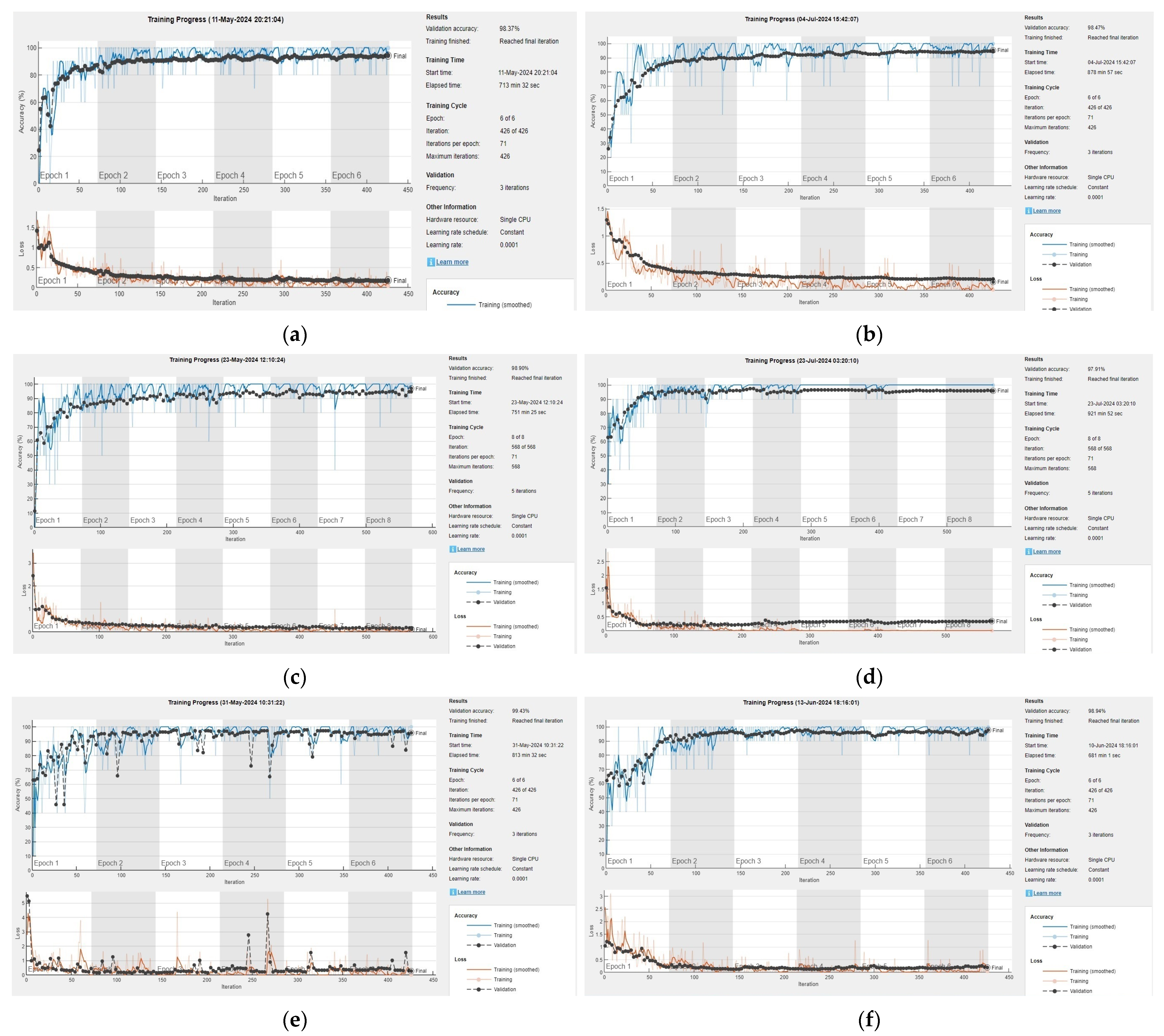Figure 10 shows the accuracy graphs of the six different deep learning architectures used in the study.

In the study, the same data set was used to minimize the error rate. Image sizes were changed according to deep learning architectures. Training times and accuracy rates change according to deep learning models. The shortest training time was 681 min in the Xception architecture. The longest training time was 921 min in the ResNet101 architecture. The difference between the shortest and the longest time is 140 min. The accuracy rates of the study varied between 98.375% and 99.435%. The highest was 99.435% in the ResNet101 architecture and the lowest was 98.375% in the AlexNet architecture. There was a 1.060% difference between the accuracy rates. In the study, the ResNet101 architecture, which gave the highest accuracy rate, was used.

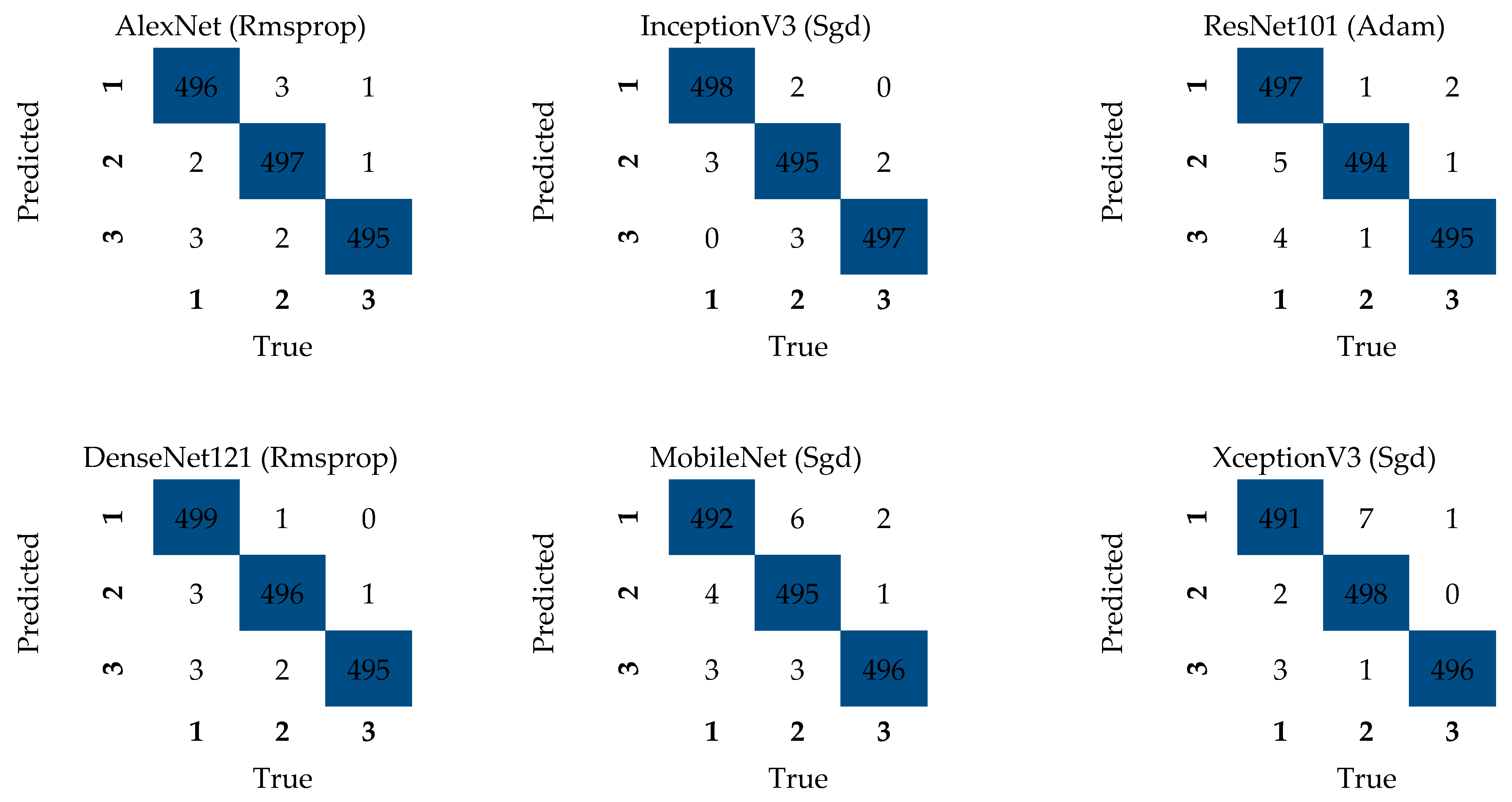
Complexity matrices provide a pictorial representation of precision and recall information on a class-by-class basis. It is used to see how many of the predictions made for each class are correct and how many are wrong. Figure 11 shows the complexity matrices for the six different models tested in this study.

For the complex matrix, 500 examples from each class were used. These examples were used in the same way in six different deep learning architectures. In this way, the error rate was minimized. A total of 1500 tests were performed on each architecture. There was a very small difference in the accuracy rates of all models. However, the accuracy rates were higher than 99% in all models. The test results and the results after optimization show very close values.

A second data set was prepared to verify the success of the models of the study. This data set consists of images taken from a different terrain. When the images in the second test set are examined, it is seen that there are too many weeds. Despite these, the accuracy rates obtained were quite high.

Table 3. Loss, accuracy, precision, sensitivity, and F1 scores were obtained in the second test set.

Optimization Method
Models	Lost	Truth	Precision	Recall	F1 Score
AlexNet (Rmsprop)	0.0903	85.72	0.87	0.84	0.82
InceptionV3 (Sgd)	0.9503	85.37	0.89	0.85	0.83
ResNet101 (Adam)	0.8509	87.93	0.91	0.88	086
DenseNet121 (Rmsprop)	0.9716	80.13	0.81	0.79	0.74
MobileNet (Sgd)	0.8412	81.59	0.85	0.82	0.80
Xception (Sgd)	0.6848	86.51	0.88	0.87	0.84

shows the loss, accuracy, precision, sensitivity, and F1 scores obtained in the second test set.

In the second test set, the highest accuracy value was obtained as 91.27% with the ResNet101 model and the Adam optimization method.

Accuracy rates were increased by applying different filters to the first and second data sets.

Table 4. Loss, accuracy, precision, sensitivity, and F1 scores were obtained in the first and second test sets.

Applied Filter	Models	Truth First Test	Truth Second Test	Truth Average
	AlexNet	93.19	76.80	84.99
	InceptionV3	99.15	84.32	91.73
	ResNet101	93.17	77.96	85.56
	DenseNet121	99.71	86.69	93.26
	MobileNet	99.77	81.37	90.57
	Xception	99.80	88.45	94.12
Median (3 × 3)	AlexNet	92.95	77.13	85.04
	InceptionV3	99.67	84.21	91.94
	ResNet101	91.95	79.08	85.51
	DenseNet121	99.81	92.95	96.30
	MobileNet	99.70	81.51	90.60
	Xception	99.95	88.85	94.40
Median (7 × 7)	AlexNet	94.96	77.85	86.40
	InceptionV3	99.81	89.54	94.67
	ResNet101	92.11	77.18	84.6
	DenseNet121	99.81	87.15	93.48
	MobileNet	99.79	81.80	90.79
	Xception	99.89	88.38	94.08

shows the accuracy rates after the filters were applied to the first and second data sets.

When only the high-pass filter was applied, 99.80% accuracy was achieved with the Xception model for the first test set, and 88.45% accuracy was achieved with the Xception model for the second test set. When the median (3 × 3) process was applied after the high-pass filter, 99.95% accuracy was obtained with the Xception models for the first test set, and 88.85% accuracy was obtained with the DenseNet121 model for the second test set. When the median (7 × 7) process was applied after the high-pass filter, 99.89% accuracy was obtained with the Xception models for the first test set, and 88.38% accuracy was obtained with the InceptionV3 model for the second test set.

As a result of the studies, the best result on average was achieved in the InceptionV3 architecture.

4. Discussion

When the literature studies are examined, it can be seen that many studies have been performed. In these studies, different data sets were prepared. There are differences in the number of photographs that make up the data sets. Different architectures were used in the classification process. In this way, different accuracy rates were obtained.

Table 5. Comparison of the literature.

Writer	Herb	Architectural	Accuracy Rate (%)
Mahum et al. [20]	Potato	Efficient DenseNet CNN	97.60
Arya and Rajeev [21]	Potato	CNN and AlexNet	97
Sarker et al. [22]	Potato	ResNet50 CNN	98.90
Islam et al. [23]	Potato	Support vector machines (SVMs)	97
Wang et al. [24]	Potato	VGG16 CNN	84
Park et al. [25]	Potato	VGG16 CNN	91
Vijayalata et al. [26]	Cassava	EfficientNet-B0 CNN	83
Feriates et al. [27]	Cassava	SVM	99.70
Periya et al. [28]	Cotton	Faster R-CNN	94
Whang et al. [29]	Apple	VGG16 CNN	86
Kukreja et al. [30]	Potato	CNN	86.39
Park et al. [31]	Apple	CNN	99
Eser et al. [32]	Potato	Faster R-CNN	98.92
Asif et al. [33]	Potato	CNN	80
Hang et al. [34]	Potato	VGG16	91
Habib et al. [35]	Jack fruit	K-means and linear SVM	92.92
Kumar et al. [36]	Tomato	Firefly algorithm, whale-optimization-based ANN	96.75
Baharvaga et al. [37]	Banana	SVM, ANN, KNN	95.72
Doh et al. [38]	Citrus	K-means, ANN, SVM	93.12
Kumari et al. [39]	Mango	Fuzzy K-means, GLCM, PCA, backpropagation	98.40

shows the comparison of literature studies.

As a result of the literature review, it is understood that it is quite difficult to use the previously made systems in daily life. The systems made only focus on objects in a certain place. In this case, it causes very low or no detection of different objects. In other studies, classification is carried out in a laboratory environment. The accuracy rate is high in this type of application. However, real-time applications cannot be made.

Since the system in this study will be used in real life, the data set must be prepared very well. For this purpose, the data set was prepared according to three important rules. These are: different locations, different light conditions and levels, and finally different distances. When looking at the data sets in literature studies, they are very small. When a real-time detection is to be made, the data set must be large. At the same time, all kinds of photographs must be in the data set. For this purpose, samples were taken from potato plants located in different locations in real life in the study. Images of the potato plants were taken in different light conditions and at different height levels. For this purpose, images of the potato plants were taken at different times of the day. Finally, images were taken from different distances. A data set was created thanks to these images. The more suitable the data set is for real life, the more accurate the detection process is. For this purpose, different operations were performed on the data set. The first of these was that different filters were applied to the data set. Finally, real-time detection was carried out with a drone camera. All errors that may occur in the camera were applied to the images in the data set. In this way, 99.81% accuracy was achieved.

Detection operations have been performed for many different types of diseases in the literature. The accuracy rates, which were very low in the first studies, have increased over time. When we look at the latest studies, the highest accuracy rate of 99.70% was achieved. In the study, an accuracy higher by 0.11% was achieved.

5. Conclusions

In this study, potato beetles found on potato plants were successfully detected using deep learning methods. High accuracy rates were obtained in the classification study carried out with six different deep learning models. Thanks to the deep learning models used, potato beetles can be detected quickly, easily, and with high accuracy. Images were taken of two different fields in the study. A data set was created with the images taken of the first field. Grayscaling, adding noise, blurring, rotating left and right, increasing and decreasing brightness, cropping, horizontal rotation, and clockwise and counterclockwise rotation operations were applied to all photos in the data set. In this way, the data set was both enlarged and precautions were taken against errors that may occur from the camera. The created data set was used in six different deep learning architectures and three different optimization methods. As a result of the study, the highest accuracy was obtained in the ResNet101 architecture and the Adam optimization method. The accuracy rate was 91%. Then, 3 × 3 and 7 × 7 filtering processes were performed to increase the accuracy rates of the study. The filtering process was first applied to the data set consisting of photos taken of the first field. The accuracy rates in this data set were very high. To prove the accuracy of the study, a second data set was created with photographs taken of the second field. This data set was used only for testing purposes. Six different architectures achieved lower accuracy rates in the second data set. As a result of the study, Xception achieved the highest accuracy rate with 99.95% in the first data set. DenseNet121 architecture achieved the highest accuracy rate with 92.95% in the second data set. The highest average accuracy rate was 96.30% in the DenseNet121 architecture.