Abstract
The modular reconfigurable flight array (MRFA) is composed of multiple identical flight unit modules, which has several advantages such as structural variability, strong versatility, and low cost. Due to the redundant properties of MRFA, it keeps stable by adopting a suitable control law when it suffers actuator fault or actively stops some actuators. To address the attitude stability issue of the modular flight array when actuators actively stop or encounter failures during the flight process, a modeling method based on a switched system is proposed at first, and an arbitrary switched controller design method based on the segmented Lyapunov functions and the average dwell time is also given. By introducing the actuator efficiency matrix, the dynamic switched model of the modular flight array is described. Then, a group of arbitrary switched linear feedback gains is designed to ensure the exponential stability of the flight array if the switched process satisfies the constraint of the average dwell time. Simulation and experiment results indicate that when there is an accident in the actuator states, the switched controllers can achieve precise tracking of the desired trajectory, thus confirming the effectiveness of the proposed modeling method and controller.
1. Introduction
In recent years, a variety of unmanned aerial vehicles (UAVs) have been proposed to be adapted to complex dynamic environments or to undertake more challenging missions [1]. Many concepts such as UAV swarms that collaborate with multiple unmanned aerial vehicles [2], omnidirectional heterogeneous UAV [3], coaxial drones [4,5], multi-modal drone with three different flight modes (rotor wing, tailsitter, cruise) [6], and MRFA [7,8,9,10] have also emerged. The multi-linked aerial robot, named DRAGON, described in reference [7], incorporates a two-degree-of-freedom (DoF) force vectoring apparatus in each link. This aircraft connects individual flight modules through a flexible swinging motion framework, enabling the aircraft to possess the capability to flexibly change its configuration during flight. Reference [8] proposes a novel modular design-based reconfigurable transport drone that can adapt to the shape, size, and weight of payloads, thus avoiding the lack of flexibility in traditional drones, which require updating specific cargo dimensions to customize different drone fleets. References [9,10] introduce another novel modular aircraft for distributed flight array systems. The flight system is capable of aerial configuration reconstruction, cooperative transportation, and self-reconfiguring fault tolerance in the event of system failures. Among those different types of UAVs, the MRFA has certain advantages for its variable structure and higher environmental adaptability. It is composed of several standard and common flight modular. Different MRFA configurations can be rapidly constructed by assembling multiple universal modules to fit for various mission requirements and environmental constraints. Consequently, MRFA has promising applications on complex environments and multiple mission scenes.
When an MRFA possesses no less than four universal flight modules, stable flight can be achieved in the event of actuator deactivation or actuator failure by full use of the redundancy of actuators. This feature enhances the resilience and versatility of the MRFA, and then improve its fault-tolerant capability.
In addressing the fault-tolerant control challenges of rotorcraft, comprehensive and systematic research has been conducted by scholars [11,12]. In [11], an adaptive control strategy is proposed to estimate the fault parameter of the actuator, with which the stabilization problem of the quadrotor with actuator fault can be effectively solved. Reference [12] compares the static hover of two different configurations of hexacopters (coaxial Y-shaped and regular hexagonal) when one actuator fails. Following the geometric interpretation, it demonstrates that the hexacopter with a hexagonal configuration is unable to maintain static hover when one of its propellers fails, whereas the Y-shaped hexacopter can maintain static hover even when any one propeller fails. The control allocation technique, which is widely used in UAV is applied in [13], wherein the control signals of UAV actuators are directly reassigned to the remaining properly functioning actuators. This approach achieves fault redundancy without altering the control laws of the UAV. In [14], a gain scheduling mechanism based on PID control is devised, involving the design of multiple PID controllers to address the fault-tolerant control issues of a quadrotor under normal operation and in the event of different actuator failures. Through gain scheduling, the UAV undergoes flight mode switching from normal flight to the occurrence of actuator failures, ultimately endowing the UAV with fault tolerance. However, due to the disparate control gains associated with the UAV in different states, the stability problem of the UAV control system at controller switching time can not be guarantee from theoretical prospects. This drawback may result in a degradation in UAV stability performance or even attitude instability. In [15], a robust optimization approach is used to deal with uncertain power outputs, which can be used to solve the problem of abrupt energy output in the event of actuator failure in multi-rotor UAVs.
Considering the inherent property of actuator redundancy in MRFA and the practical demand for fault-tolerant control of UAVs, an attitude control method of MRFA based on the switched control approach is proposed. This approach ensures the stability of MRFA during modal transitions triggered by actuator deactivation or actuator failure. This ensures exponential stability under any switched law, realizing stable flight during mode transitions. The aim of this paper is to investigate control strategies for redundant actuator systems. In MRFA systems, traditional control methods may not effectively address actuator failures. To tackle this issue, a design scheme based on dwell time arbitrary switching systems is proposed in this paper. According to pre-defined switching rules, the controllers are automatically switched in the event of actuator failures to maintain the stability and flight performance of the MRFA. The paper is organized as follows: Section 2 provides a brief description of the mechanical design and optimization of the MRFA, Section 3 elaborates on the mathematical model of the MRFA, and Section 4 introduces the MRFA switched controller and its design methodology. The effectiveness of the designed switched controller is verified through numerical simulations and experiments in Section 5, accompanied by details on the hardware setup of the experimental platform and its structure. Finally, conclusions are drawn in Section 6.
2. Design of the Mechanical System
MRFA is assembled by arbitrarily combining multiple structurally identical flight modules. Each flight module comprises components of carbon fiber panels, brushless motors, propellers, communication modules, and mechanical connectors. The connection between multiple flight modules is achieved through bolt-fastened connector components (Figure 1). It allows for the adjustment of the quantity and spatial positioning of modules based on mission requirements, ensuring that a wider array of complex and dynamic tasks can be accomplished. Through the arbitrary combination of flight modules, various configurations of the aircraft can be assembled, significantly expanding the functionality and application scenarios beyond traditional aircraft. To facilitate dynamic modeling and control design, we assume that all flight modules are uniform, including shape, mass, inertia, and actuators.
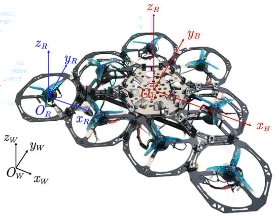
Figure 1.
Coordinate schematic of modular reconfigurable flight array (MRFA). The earth coordinate frames, module coordinate frames, and flight array coordinate frames are represented by the black, red, and blue axes, respectively.
3. Modeling of MRFA
3.1. Coordinate Frames
Three different coordinate systems are employed for describing the positional relationships between flight modules and the MRFA. The three coordinate systems shown in Figure 1 are defined as follows.
The earth coordinate frame W: or inertial coordinate system, is characterized by adherence to the right-hand rule, with its three axes following the convention of the East–North–Up direction. The position of the MRFA in the earth coordinate system is denoted by . The attitude of the MRFA is denoted by , where represent the roll, pitch, and yaw angles, respectively.
The flight module coordinate frame : representing the position of each individual flight module. corresponds to the coordinate system of the i-th flight module, where the subscript . The origin of the coordinate system coincides with the center of mass of the flight module. The z-axis aligns with the thrust direction generated by the propellers. For model simplification, it is assumed that the x-axis of all flight modules points in the same direction.
The structure coordinate frame B: The origin of the coordinate system is positioned at the center of mass of the MRFA, adhering to the right-hand rule. The x-axis aligns with the forward direction of the MRFA, and the z-axis is oriented vertically upward from the horizontal plane of MRFA.
3.2. Dynamic Model of the MRFA
The dynamic model of the MRFA is employed to describe the relationship between the forces and torques acting on the UAV array and its motion. The modeling approach in [16] is adopted, assuming equal mass for each flight module. Based on the relationships between lift, torque, motor speed, and control channels, a generalized and universal dynamic model for the irregularly structured MRFA is established, as presented below.
The kinematic equations can be expressed as:
where N represents the number of modules in the MRFA, m denotes the mass of a single module, , T represents the resultant force exerted on the MRFA in the structure coordinate system.
Based on the inertia matrix of a single flight module , using the parallel axis theorem, once the MRFA is determined, the relationship between MRFA and the rotational inertia can be established.
where and denote the positions of the geometric centers of each flight module in the structure coordinate system. Equation (2) can be rearranged as:
Its inverse matrix is given by:
where
The rotational motion of the MRFA can be given as
where represents the rotational torques exerted on the MRFA due to rotation about the , and axes of the structure coordinate system.
where k represents the rotation direction of the propellers in the MRFA, with when the blade rotates clockwise and when the blade rotates counterclockwise.
To further simplify the model, it is assumed that the MRFA satisfies the small angle assumption [17], and nonlinear terms such as aerodynamic damping are neglected. Therefore, the simplified model of the MRFA is represented by
To achieve the attitude control of the MRFA, it is necessary to establish the error-dynamic equations based on the mathematical model of the MRFA. For each switching subsystem, we design a feedback gain matrix to ensure that the states of each subsystem quickly track the reference signal.
Define as the reference signals. The tracking error states are , , , , , , , . Substituting Equations (7) and (8), the error-dynamic equations of the MRFA can be expressed as follows:
The error-dynamic equations are represented in state–space form as follows:
where
3.3. Control Allocation
The MRFA generates lift and torque by driving the propeller blades to rotate through motors, enabling motion in various directions. As there are no actuators directly generating thrust and torque in the system, the thrust produced by the motors is considered as the input vector for the actuators, and the input to sustain the motion of the flight array is treated as a virtual control input vector. Figure 2 illustrates the schematic structure of control allocation in the control system.
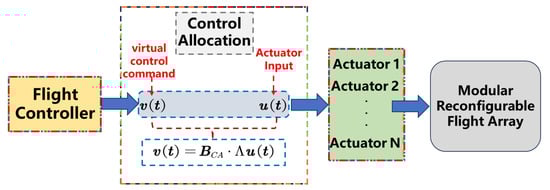
Figure 2.
Control allocation.
Control allocation reasonably and uniquely assigns the virtual control commands corresponding to the control laws to each actuator, in order to obtain the desired control performance. The relationship between virtual control input and the actual input to the actuators is expressed by the following equation:
where represents the actual inputs to the actuators of the MRFA, represents the virtual control input, and is the control allocation matrix, reflecting the mapping relationship between virtual control input and actual input.
For quadrotor, the pulse width modulation output signal u from the electronic speed controller is approximately proportional to the square of the speed of the brushless motor [18]. The lift and torque of the flight unit module are proportional to the square of the rotor speed [19]. Details of the relationship can be seen in Equation (12).
where p is the proportional coefficient, represents the speed of the brushless motor, is the lift coefficient, and is the torque coefficient.
The characteristic of the arbitrary interconnection and variable structure among flight modules in the MRFA allows for various configurations. When substituting the control allocation matrix into Equation (11), the following equation is obtained.
where .
In accordance with Equation (13), the values of the control allocation matrix are solely dependent on the distribution of actuators within the MRFA and the rotation direction of the propellers. Based on the positional information of each module and the rotation direction of the propellers, the control allocation matrix for the corresponding MRFA can be determined (Figure 3). The red arrow indicates counterclockwise rotation of the propeller, while the blue arrow indicates clockwise rotation of the propeller. The Moore–Penrose pseudoinverse ultimately is employed to allocate the virtual control commands to each actuator. One has
where represents the right pseudo-inverse of the control allocation matrix .
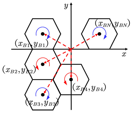
Figure 3.
The distribution of modular position.
Remark 1.
The mixer matrix of the MRFA is a matrix used to convert the control inputs of the aircraft into speed commands for each actuator. From Equation (14), it can be derived that the rotor speeds of the actuators can be obtained through the control inputs of the flight array transformed by matrix , thus inferring the equivalence between the mixing matrix and matrix .
4. Arbitrary Switched Controller Design
To ensure robust control performance when no less than one actuator suffers an accident and has to switch to alternative actuator combinations, a switching controller is designed to accommodate the arbitrary switching law. To characterize the controllability of the MRFA in the presence of faults or failures in the power system, a diagonal matrix is introduced to depict the states of each rotor.
where denotes the actuator state matrix. Here, indicates a complete failure of the l-th motor; signifies a partial failure of the actuator; represents the full health of the actuator. Consequently, the error-dynamic equation of the MRFA, encompassing the actuator states, can be derived:
where denotes the control allocation matrix with actuator states.
When a failure of actuator occurs, the actuator state matrix undergoes changes. A linear switched system with actuator fault can be described as Equation (16).
where the switching law is a right-continuous constant function with time t as a variable. In the time sequence , when , represents the activation of the p-th system, corresponding to the selection of the system matrix .
Remark 2.
When the number of flight modules in the MRFA is more than 4 (), the MRFA, as an actuator redundant system, has a subset of actuators , where , which is mainly used to enhance and improve the performance of the actuators. If a failure occurs in these actuators, it will not affect the stability of the system. Another subset of actuators can affect the stability of the system if a failure occurs, making the system lack fault tolerance. In an MRFA, when the control allocation matrix containing the state of the actuators is less than full rank, the corresponding set of actuators belong to . For ease of study, we consider the system switching among controllable combinations of actuators. That is, the actuator combination of MRFA belongs to .
According to the description mentioned above, MRFA is easy to facilitate redundant control. When certain actuators proactively cease operation or encounter failures, a fault-tolerant switched controller is designed based on segmented Lyapunov methods [20]. This method can keep stable flight during mode transitions in the MRFA.
Lemma 1.
A positive number is considered as the average dwell time if there exists a switching signal and the number of switches during the time interval , such that a non-negative integer is satisfied [21].
Theorem 1.
For the MRFA satisfying the switched model in (17), if for each switched subsystem, there exists a state feedback controller
where the feedback gain of the controller is ,, is a positive definite matrix for subsystem i, positive numbers , and are chosen such that the following matrix inequalities hold:
And the average dwell time satisfies
The system can be exponentially stabilized under arbitrary switched law.
Proof of Theorem 1.
For each subsystem of the switched system in MRFA, the following piecewise Lyapunov function is defined:
where the positive definite matrix satisfies the matrix inequalities (20) and (21). When the MRFA switches to the i-th subsystem, the time derivative of is given by:
Substituting the error state space (Equation (16)) into the above equation, we obtain:
Rearranging the equation by substituting the state feedback controller (19), we obtain:
Then, we have
Assuming that the switching signal of each subsystem in the MRFA satisfies , the result from Equations (20) and (29) can be obtained as follows:
Then,
Therefore, for each subsystem of the MRFA, given the satisfaction of the average dwell time with Equation (30), it can be inferred that upon exiting the previous subsystem, the Lyapunov function value of the current subsystem at the current moment is less than the Lyapunov function value of the last activated subsystem. Hence, the MRFA switched system is exponentially stable under the condition of satisfying the average dwell time (22). □
To obtain the switched controller, let and . By left-multiplying and right-multiplying both sides of Equation (20) with and both sides of Equation (21) with , we obtain:
By using the Schur complement, the above equation is equivalent to:
5. Experiments
5.1. Simulation
Considering the MRFA with eight modules shown in Figure 4, the tracking performance of the proposed switched control algorithm for reference trajectories is evaluated through numerical simulation and experimental testing under scenarios with no actuator failure, failure of actuator 5, and failure of actuators 1 and 4.
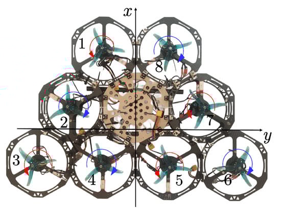
Figure 4.
Modular reconfigurable flight array (MRFA) with eight modules.
The relevant parameters of the flight module (as shown in Table 1) can be used to compute the physical parameters of the MRFA, as depicted in Figure 4. Subsequently, the values for and in the expression for the error tracking state space (16) can be determined.

Table 1.
Parameters of flight module.
The position information of each module is computed based on the edge length information of the MRFA unit module. The lift coefficient , the torque coefficient , and the proportionality coefficient [17]. With this information, the MRFA control allocation matrix can be determined:
Remark 3.
Due to the fact that and are functions of the propeller’s radius, geometry, and air density, the chosen dimensions of the propeller in this experiment are the same as those in reference [17]. However, due to differences in air density and propeller geometric shape during experiments, the output of the actuators can be adjusted by introducing positive constant matrices β and ζ. The corrected MRFA actuator output can be expressed as
where the symbol ∗ denotes the Hadamard product. The actuator output consists of two terms: the first term is related to the state of the flight array, and the second term is related to the desired attitude trajectory of the MRFA. It can be used to suppress the oscillation of the actuator output. By adjusting the constant matrices β and ζ, the proportion of these two terms can be adjusted.
Sequentially we compute the control allocation matrices , , where , and represent the control allocation matrices when there is no actuator failure, actuator 5 fails, and actuators 1 and 4 fail, respectively.
The parameters are set as , , , , , and an LMI solver is utilized to solve Equations (33) and (34) to obtain matrices and . From these, we derive the positive definite matrices and corresponding to scenarios with no actuator failure, actuator 5 failure, and actuators 1 and 4 failure, respectively.
Remark 4.
The process of solving the LMIs mentioned above is performed offline on a ground station, utilizing the Python programming language for implementation and storing the results. If an onboard computer is installed on the reconfigurable flight array, LMIs can be solved online, and the controller gains can be determined accordingly. Finally, the results can be transmitted to the flight controller via USB communication, which will be implemented in future work.
Let , from Equation (22), we obtain . When the dwell time , the switching signal is illustrated in Figure 5.
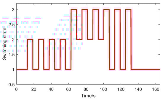
Figure 5.
The switching laws of modular reconfigurable flight array (MRFA).
The MRFA has three states. When , it indicates that the MRFA is in a fault-free state. For , the fifth actuator is faulty. When , the first and fourth actuators are faulty. Calculating the controller feedback gains yields:
The computed feedback gains are substituted into Equation (19), resulting in arbitrary switched controllers for the MRFA with eight modules, as depicted in Figure 4, under scenarios without actuator faults, with a fault in the fifth actuator, and with faults in the first and fourth actuators.
Trajectory tracking of the MRFA’s attitude angles (roll, pitch, and yaw) yields the simulation results depicted in Figure 6.
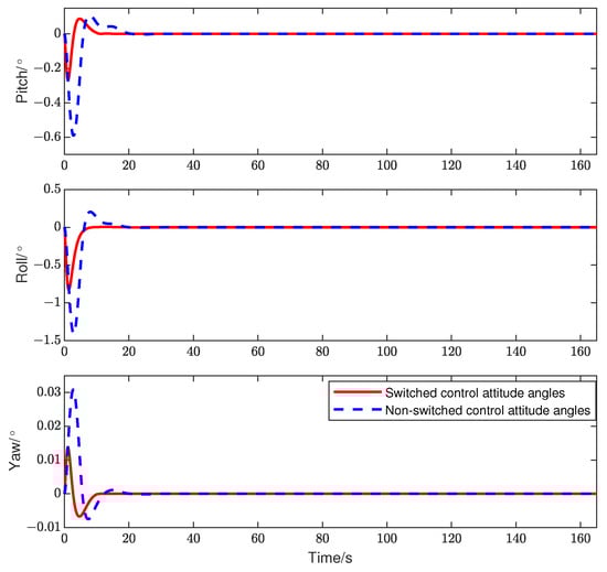
Figure 6.
Comparison of attitude tracking curves between switched controller and non-switched controller.
From Figure 6, it can be observed that the error curves for the MRFA with the configuration shown in Figure 4 are convergent both without controller switching and under the switching law depicted in Figure 5. However, the error curve for the switched control based on the law in Figure 5 is smoother and converges faster. In the case of actuator failure, the error curve without switched control exhibits significant overshooting, and the convergence time of the error curve is longer compared to the error curve with the addition of switched control, as illustrated by the blue dashed line in Figure 6. In the event of actuator failure, the switched control based on dwell time needs to redistribute the power loss caused by the failed actuator to the remaining functional actuators, thereby reducing the sudden change in tracking error.
Therefore, the simulation validates the effectiveness of the arbitrarily designed switched controller for the MRFA.
5.2. Experiment
In this subsection, the attitude stability of the MRFA is experimentally investigated using a three-degrees-of-freedom testbed. The attitude control frequency of the MRFA is set to 200 Hz, and the IMU sensor update frequency is 1000 Hz. The experimental platform is shown in Figure 7.
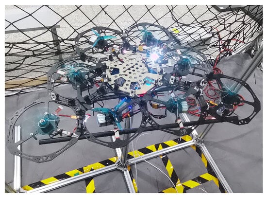
Figure 7.
Three-degrees-of-freedom testbed.
The MRFA utilizes an Ano flight controller developed by an Anonymous technology startup as the controller. The flight controller is equipped with an STM32F407VGT6 microcontroller, with a maximum frequency of up to 168 MHz, and employs an ICM20602 IMU sensor produced by the Japanese electronic component manufacturer TDK to measure the attitude information of the flight array. The actuators of the flight array are Tmotor F80Pro brushless DC motors, manufactured by the Tmotor brushless motor manufacturer, and powered by a 4S lithium battery.
The MRFA is connected to the three-degrees-of-freedom test bed using custom connectors, restricting the translational motion of the MRFA. To validate the effectiveness of the switched controller, both the switched controller and the cascaded Proportional-Integral-Derivative (PID) controller were employed for attitude trajectory tracking control of the MRFA. To ensure comparability between the two controllers, PID parameters were selected to match the tracking curves of both controllers in the absence of actuator faults. The PID parameters are listed in Table 2.
Table 2.
Proportional-Integral-Derivative parameters of modular reconfigurable flight array (MRFA).
When conducting attitude trajectory tracking with the switched controller, adjustments were made to track the reference trajectory, considering the simplified linear model of the MRFA model and the fact that the lift coefficient and torque coefficient of the experimental platform’s propellers differed from the coefficients in [17]. This was achieved by introducing the adjustment coefficient matrices and .
According to the switching law shown in Figure 5, attitude trajectory tracking control was performed on the MRFA for each case, as illustrated in Figure 8.
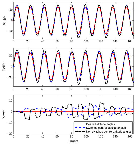
Figure 8.
Comparison of attitude tracking curves at arbitrary switched controller and non-switched controller.
The red curve in Figure 8 represents the reference attitude trajectory of the MRFA, the blue dashed line represents the attitude tracking curve under the arbitrary switching controller, and the black dashed line represents the attitude tracking curve without using the switched controller. Under the switching law in Figure 5, for the MRFA with no actuator failure during the time intervals 0 s ≤ t ≤ 15 s and 132 s < t ≤ 165 s, the tracking curves under the two different control strategies overlap substantially. During the transitions of the MRFA to states and , where actuator 4 continuously switches between healthy and completely failed states, the attitude tracking curves under the switched controller and without the switched controller can both follow the reference curve. However, the tracking curve under the switched controller is closer to the reference curve, because the switched controller can dynamically adjust the control strategy based on the current system state to adapt to different flight conditions. When some actuators in the MRFA fail or malfunction, the switched controller can promptly adjust the control strategy, redistribute power, allowing the system to maintain a stable flight state and get closer to the reference trajectory. When the MRFA transitions to state , where both actuators 1 and 5 simultaneously suffer complete failure, the lost power of the MRFA cannot be compensated by the PID controller within a short time. This results in a situation where the remaining actuators are insufficient to precisely track the reference attitude curve, leading to a sudden increase. In contrast, for systems utilizing the switched controller, when an actuator failure occurs, the control gains of each actuator can be switched to redistribute the outputs of each actuator, as illustrated in Figure 9. This enables the rapid convergence of tracking errors in the MRFA. As a result, the system can quickly adapt to the new power distribution and ensure rapid convergence of the MRFA’s tracking error. Therefore, employing a switching controller can enhance the fault tolerance of the MRFA against actuator failures, ensuring system stability and performance.
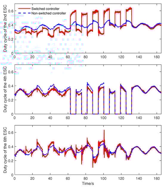
Figure 9.
The partial actuator output curve of modular reconfigurable flight array (MRFA).
When employing different control strategies, the outputs of the actuators also undergo changes. Under the switching law depicted in Figure 5, the partial actuator output curves of the MRFA during pitch angle trajectory tracking are illustrated in Figure 9. When a state transition occurs and an actuator fails, there is an instantaneous reduction in power, leading to a sudden change in tracking error. Therefore, the actuator outputs under the two control strategies used in this paper exhibit abrupt changes. The blue dashed line corresponds to the case without using the switched controller is smoother compared to the curve with the switched controller. This is due to the fact that the arbitrary switched control redistributes the power loss caused by actuator failure due to the remaining properly functioning actuators.
From Figure 9, it can be observed that the behavior of actuators with different indices varies during the occurrence of actuator failures in the MRFA. In the configuration of the MRFA shown in Figure 4, between 15 s < t ≤ 63 s, the MRFA switches back and forth between states and . When the MRFA tracks the reference pitch angle curve, actuator 2 is located in the positive half-axis of the body coordinate system’s x-axis, and actuators 4 and 6 are in the negative half-axis of the x-axis. Since the four actuators in the negative half-axis of x generate smaller torques along the y-axis to ensure precise pitch angle tracking after the failure of actuator 5, the output of actuator 2 needs to decrease, while the outputs of actuators 4 and 6 need to increase. During the time interval 63 s < t ≤ 132 s, when , actuators 1 and 4 fail. Therefore, the output of actuator 4 is 0 when . In the process of switching back and forth between states and , the MRFA is always in a state where the actuators cannot work completely. As shown in Figure 9, for any switched control strategy, the actuator undergoes the maximum mutation amplitude at this point, facilitating the redistribution of power to achieve precise tracking of the reference attitude.
6. Conclusions
If there is a failure in the actuators of the MRFA, the instantaneous reduction in power may cause a sudden change in tracking error. In addressing the issue of partial actuator failures in the MRFA, a modeling approach based on a switched system is proposed. Furthermore, a robust arbitrary switched controller design method is introduced. When the MRFA suffers partial actuator failures, it is necessary to design a state feedback controller for each subsystem that satisfies arbitrary switching. This controller enables the MRFA to keep better stable performance if the actuators have to switch arbitrarily among different combinations of actuators. The proposed method ensures that the MRFA can mitigate or eliminate disturbances caused by actuator failures through switching, thereby achieving rapid tracking of the desired trajectory. We conclude our results as two points.
1. Through simulation and experimental validation, we have found that compared to the cascade PID controller, the proposed control strategy based on dwell time can achieve more accurate attitude trajectory tracking in the presence of multiple actuator failures.
2. Under the two control strategies used in this work, the outputs of the actuators will experience sudden changes. The main differences between two methods is that the output generated by the cascade PID controller is smoother than that of the switched controller. It means that the cascade PID controller does not compensate power loss by actuator fault while the switched controller does. Therefore, the method based on the dwell time switching controller can achieve more accurate attitude trajectory tracking in the presence of multiple actuator failures.
In practical applications, actuator faults in the MRFA may significantly deteriorate system performance, so timely identification and handling of actuator fault are crucial. Therefore, our future work may introduce fault detection of the actuator into the control strategy to enhance the robustness and reliability of the MRFA system against actuator faults.
Author Contributions
Conceptualization, C.Y.; software, B.R.; writing—original draft, B.R.; writing—review and editing, C.Y., W.M. and X.Z.; supervision, C.Y. All authors have read and agreed to the published version of the manuscript.
Funding
This work is supported by the National Nature Science Foundation under Grant 62063011, 62303199, Yunnan Major Scientific and Technological Projects under Grant 202202AG050002, 202302AD080005, Yunnan Fundamental Research Projects (Grant No. 202301AT070401) and partially supported by the Scientific Research Project of Yunnan Provincial Department of Education (Grant No. 2023Y0418).
Data Availability Statement
All data generated or analyzed during the study are included in this published article.
Conflicts of Interest
The authors declare no conflicts of interest.
References
- Saeed, A.S.; Younes, A.B.; Cai, C.; Cai, G. A survey of hybrid unmanned aerial vehicles. Prog. Aerosp. Sci. 2018, 98, 91–105. [Google Scholar] [CrossRef]
- Zhou, X.; Wen, X.; Wang, Z.; Gao, Y.; Li, H.; Wang, Q.; Yang, T.; Lu, H.; Cao, Y.; Xu, C.; et al. Swarm of micro flying robots in the wild. Sci. Robot. 2022, 7, Eabm5954. [Google Scholar] [CrossRef] [PubMed]
- Park, S.; Lee, J.; Ahn, J.; Kim, M.; Her, J.; Yang, G.H.; Lee, D. Odar: Aerial manipulation platform enabling omnidirectional wrench generation. IEEE/ASME Trans. Mechatron. 2018, 23, 1907–1918. [Google Scholar] [CrossRef]
- Schafroth, D.; Bermes, C.; Bouabdallah, S.; Siegwart, R. Modeling, system identification and robust control of a coaxial micro helicopter. Control Eng. Pract. 2010, 18, 700–711. [Google Scholar] [CrossRef]
- Pastor, D.; Izraelevitz, J.; Nadan, P.; Bouman, A.; Burdick, J.; Kennedy, B. Design of a ballistically-launched foldable multirotor. In Proceedings of the 2019 IEEE/RSJ International Conference on Intelligent Robots and Systems (IROS), Macau, China, 3–8 November 2019; pp. 5212–5218. [Google Scholar]
- Sufiyan, D.; Win, L.S.T.; Win, S.K.H.; Pheh, Y.H.; Soh, G.S.; Foong, S. An Efficient Multimodal Nature Inspired Unmanned Aerial Vehicle Capable of Agile Maneuvers. Adv. Intell. Syst. 2023, 5, 2200242. [Google Scholar] [CrossRef]
- Zhao, M.; Okada, K.; Inaba, M. Enhanced modeling and control for multilinked aerial robot with two dof force vectoring apparatus. IEEE Robot. Autom. Lett. 2020, 6, 135–142. [Google Scholar] [CrossRef]
- Mu, B.; Chirarattananon, P. Universal Flying Objects (UFOs): Modular Multirotor System for Flight of Rigid Objects. IEEE Trans. Robot. 2019, 36, 458–471. [Google Scholar] [CrossRef]
- Oung, R.; D’Andrea, R. The distributed flight array: Design, implementation, and analysis of a modular vertical take-off and landing vehicle. Int. J. Robot. Res. 2014, 33, 375–400. [Google Scholar] [CrossRef]
- Saldana, D.; Gabrich, B.; Li, G.; Yim, M.; Kumar, V. Modquad: The flying modular structure that self-assembles in midair. In Proceedings of the 2018 IEEE International Conference on Robotics and Automation (ICRA), Brisbane, QLD, Australia, 21–25 May 2018; pp. 691–698. [Google Scholar]
- Zhao, G.L.; Gao, R.S.; Chen, J.N. Adaptive prescribed performance control of quadrotor with unknown actuator fault. Control Decis. 2021, 36, 2103–2112. [Google Scholar]
- Baskaya, E.; Hamandi, M.; Bronz, M.; Franchi, A. A novel robust hexarotor capable of static hovering in presence of propeller failure. IEEE Robot. Autom. Lett. 2021, 6, 4001–4008. [Google Scholar] [CrossRef]
- Merheb, A.; Nourra, H.; Bateman, F. Active fault tolerant control of octorotor uav using dynamic control allocation. In Proceedings of the International Conference on Intelligent Unmanned Systems, Montreal, QC, Canada, 29 September–1 October 2014. [Google Scholar]
- Nguyen, D.T.; Saussie, D.; Saydy, L. Design and experimental validation of robust self-scheduled fault-tolerant control laws for a multicopter UAV. IEEE/ASME Trans. Mechatronics 2020, 26, 2548–2557. [Google Scholar] [CrossRef]
- Wei, C.; Wang, Y.; Shen, Z.; Xiao, D.; Bai, X.; Chen, H. AUQ-ADMM Algorithm-Based Peer-to-Peer Trading Strategy in Large-Scale Interconnected Microgrid Systems Considering Carbon Trading. IEEE Syst. J. 2023, 17, 6248–6259. [Google Scholar] [CrossRef]
- Yang, J.; Yang, C.; Zhang, X.; Na, J. Fixed-time sliding mode control with varying exponent coefficient for modular reconfigurable flight arrays. IEEE/CAA J. Autom. Sin. 2024, 11, 514–528. [Google Scholar] [CrossRef]
- Wang, Q.; Wang, T.; Dong, C.Y.; Jiang, W.L. Chained smooth switching control for morphing aircraft. Control Theory Appl. 2015, 32, 949–954. [Google Scholar]
- Ma, D.; Xia, Y.; Shen, G.; Jiang, H.; Hao, C. Practical fixed-time disturbance rejection control for quadrotor attitude tracking. IEEE Trans. Ind. Electron. 2020, 68, 7274–7283. [Google Scholar] [CrossRef]
- Liao, W.Z.; Zong, Q.; Ma, Y.L. Modeling and finite-time control for quad-rotor mini unmanned aerial vehicles. Control Theory Appl. 2015, 32, 1343–1350. [Google Scholar]
- Hong, X.F. Fault-Tolerant Control of Switched Systems. Master’s Thesis, Xiamen University, Xiamen, China, 2007. [Google Scholar]
- Hespanha, J.P.; Morse, A.S. Stability of switched systems with average dwell-time. In Proceedings of the 38th IEEE Conference on Decision and Control, Phoenix, AZ, USA, 7–10 December 1999; pp. 2655–2660. [Google Scholar]
Disclaimer/Publisher’s Note: The statements, opinions and data contained in all publications are solely those of the individual author(s) and contributor(s) and not of MDPI and/or the editor(s). MDPI and/or the editor(s) disclaim responsibility for any injury to people or property resulting from any ideas, methods, instructions or products referred to in the content. |
© 2024 by the authors. Licensee MDPI, Basel, Switzerland. This article is an open access article distributed under the terms and conditions of the Creative Commons Attribution (CC BY) license (https://creativecommons.org/licenses/by/4.0/).