Abstract
A new idea to deal with the backmixing problem in a scaled-up multi-inlet vortex mixer is proposed in this paper. Firstly, a Reynolds-averaged Navier–Stokes–large-eddy simulation hybrid model was used to simulate the flow field in a vortex mixer, and the numerical simulation results were compared with those from a particle image velocimetry experiment in order to validate the shielded detached eddy simulation model in the rotating shear flow. Then, by adding a series of columns in the mixing chamber, the formation of wake vortexes was promoted. The flow field in the vortex mixer with different column arrangements were simulated, and the residence time distribution curves of the fluid were obtained. Meanwhile, the degree of backmixing in the vortex mixer was evaluated by means of a tanks-in-series model. In the total ten cases related with four groups of variables, it was found that increasing the diameter of the column was the most efficient for weakening the backmixing in the vortex mixer. Specifically, the vortexes made the kinetic energy of the fluid more evenly distributed in the center of the mixing chamber, thereby eliminating the low-pressure area. After structural adjustment, the number of equivalent mixers was increased by 55%, and the peak number of residence time distribution curves was reduced from four to one.
1. Introduction
Nanocarriers are widely used in the pharmaceutical industry due to their targeted features and selective permeability [1,2]. These properties of nanoparticles can enhance therapeutic indexes [3,4] or help in the implementation of new treatments [5]. Flash nanoprecipitation (FNP) is a “bottom-up” nanoparticle assembly technology which creates a high supersaturation environment through mixing solutions, an amphiphilic polymer, and an anti-solvent together rapidly [6]. At present, this technology has been used in the production of PEGoylated nanocapsules [7], poorly water-soluble drug nanoparticles [8] and sunscreen agents [9].
FNP requires that the mixing time of the solution is lower than the nucleation and growth time of the nanoparticles. There are generally two types of mixers meeting this requirement, and they are confined impinging jets (CIJs) [10] and multi-inlet vortex mixers (MIVMs) [11]. Both of them can generate quite high local energy dissipation through the collision and reorientation of high-speed fluids. In a CIJ, the impacts between jets requires that the velocity difference in the impinging flow should not be too large to avoid the over-shifting of the stagnant point, while in an MIVM, all inlet streams contribute independently to the mixing in the chamber without a flow-rate limit. This advantage gives an MIVM greater flexibility than a CIJ, which allows it to control the solvent mixing ratio through relative flow rates [12].
As a development in MIVMs, a micro-MIVM with a diameter of several millimeters has been reported in the application of the FNP process, and it has been successfully applied in the production of nanodrugs with narrow size distributions [13,14,15]. In order to reach greater production in the fields of pesticides and cosmetics, Liu et al. [16,17,18] scaled-up this mixer and evaluated its performance by means of computational fluid dynamics (CFD) and particle image velocimetry (PIV), and they characterized the mixing performance of the MIVM using planar laser-induced fluorescence (PLIF) [19]. However, Liu et al. [16] found a significant recirculation in the center of the MIVM when the dimension of the mixer was approximately 16 times larger than the micro-MIVM studied by Cheng et al. [20]. The recirculation could potentially affect the process of particle formation, leading to a wide particle size distribution in the FNP. If the residence time of the nanoparticles in the mixer cannot be quantitatively fixed, the diameters of the particles will be uncontrollable, which will greatly compromise the performance of the product and even cause blocking in the mixer. Therefore, it is important to further develop MIVMs by solving the problem of backmixing. However, it should be noted that backmixing has not been observed in micro-MIVMs [18].
Generally, the backmixing problem can be solved by improving the internal configuration of the reactors [21], such as by adding spoilers or adjusting the shapes of the reactors. According to Liu et al.’s work [17], an MIVM is a passive mixer whose internal flow swirls with clearly curved streamlines, and it has been reported that the rotation of its fluid can affect the turbulence kinetic energy and its distribution by adding extra strain rates (such as lateral divergence, normal divergence, overall compression and rotation) to the fluid. Meanwhile, the sudden contraction of an MIVM’s outlet will also lead to lateral and normal divergence [18].
Previous studies [15,22] have demonstrated that MIVMs are valuable in mass production. For better performance in the control of the residence time distribution of a product, the backmixing problem must be resolved. To weaken the backmixing in a scaled-up MIVM, it is necessary to reduce the fluid strain at the outlet. A traditional baffle will not only change the shape of the wall and affect the flow path of the fluid but also produce a dead zone where particles are easily collected behind the baffle. Inspired by the intensified mixing induced by the Karman vortex street [23,24], we proposed a method in a scaled-up MIVM where a series of vortexes were generated around an array of columns, and they disturbed the regularity of the flow at the outlet. A computational fluid dynamics simulation was used as the main research method, which had good accuracy in calculating the convergent swirl’s flow field [25].
This paper is organized as follows: firstly, the shielded detached eddy simulation (SDES) model based on the shear-stress transport (SST) k-ω model is used to simulate the flow field in the scaled-up MIVM, and the simulation is validated by comparing the velocity field with PIV results from the literature. Then, a series of simulations are carried out based on four key variables, including the number, axis distance, diameter and rotation angle of the columns, in generating the Karmen vortex. Then, the residence time distributions are used to characterize the backmixing based on the tanks-in-series model. Further, the contours of velocity, the vorticities and the turbulence characteristics are qualitatively analyzed to identify the main cause of the backmixing. Finally, the conclusions and suggestions for future work are presented.
2. MIVM Domain and Numerical Method
2.1. Simulation Domain
Figure 1 shows a sketch of the scaled-up MIVM used in this work, and it is the same as that in Liu’s work [18]. In the operation of the MIVM, four liquid streams entered the mixing chamber from four inlets which were aligned tangentially along the chamber, and then they mixed with each other. Finally, the mixed stream flowed out of the mixer through a vertical circular outlet. The inlets were all squared in the cross-section with a width (Win) of 25.4 mm and length (Lin) of 100 mm, while the outlet had a diameter (Dout) of 25.4 mm and length (Lout) of 250 mm. The height of the mixing chamber (Hmix ) was 25.4 mm, and it had a diameter (Dmix) of 101.6 mm. The measurement plane of the PIV was located at half of the height of the mixing chamber, as shown in Figure 1b.
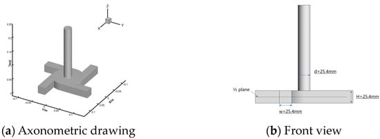
Figure 1.
Sketches of the MIVM and its dimensions.
2.2. Materials and Operating Conditions
The liquid used in the simulation was water, and its properties are shown in Table 1.

Table 1.
Physical properties of the fluid.
According to Liu et al.’s experiments [16], there was no clear relationship between the dimensionless velocity distribution near the center of the mixing chamber and the inlet’s Reynolds number, and so the velocities in the mixer could be normalized by the bulk inlet velocity. In this work, the operating conditions were consistent with those in the literature [16], where the bulk Reynolds number in each inlet was 6580 based on the inlet’s hydraulic diameter. Specifically, the average velocity of each inlet was 0.248 m/s. Boundary conditions for the velocity inlet with a zero normal gradient and pressure outlet without backflow were adopted. The walls were non-slip. Gravity was not considered. The initial pressure was a standard atmosphere.
It is known that the flow field of a Karman vortex street is related to the incoming flow velocity and column diameter [26]. Therefore, the simulations were performed as shown in Table 2, and the axis distance between the column and center (ΔL), the column diameter (φ) and their rotation angle (θ) are shown in Figure 2.
Table 2.
Variables in the simulations.
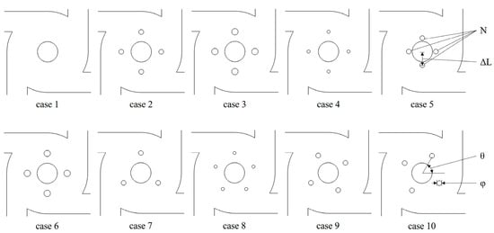
Figure 2.
Schematic diagrams of the cases listed in Table 2.
2.3. Numerical Models
When turbulent flows pass through bluff bodies, complex phenomena such as flow separation, boundary layer transition and vortex shedding occur. In addition, turbulent swirling flows exist almost everywhere in a mixing chamber. In this case, the Reynolds-averaged Navier–Stokes (RANS) model was not sufficient to capture all the details of the flow field.
Because of its advantage in balancing accuracy and efficiency in creating detailed descriptions of turbulence, the large-eddy simulation (LES) model has been popular in recent years. However, the LES model requires a high resolution grid at the wall boundary layer. In the area close to the wall, even the largest scale of the turbulence can be extremely small, and so a fine computational grid and a small time-step are required. A hybrid RANS–LES model, which combines the advantages of the RANS and LES models, could be a reasonable way to reach this balance. In such a hybrid model, the near-wall boundary layer is usually solved by the RANS part of the model, while in the separation area far away from the wall, the flow is solved by the LES model. Such hybrid models have been successfully used in describing the vortex shedding around columns [27,28].
Both the delayed detached eddy simulation (DDES) and shielded detached eddy simulation (SDES) are detached eddy simulation (DES) hybrid models. DDES models have been validated in a scaled-up MIVM [18]. However, Liu et al. [18] found that a DDES model is not perfect in its division of the RANS region and the LES region. According to the literature [29], the SDES model is better at dividing the simulation domain, which can help in further reducing the number of grids and speeding up the simulation without affecting the simulation accuracy.
The governing equations of the SDES model based on the k-ω SST model are as follows:
where F1 and F2 are the SST blending functions, μt is the turbulent eddy viscosity, Pk is the generating term of the turbulent kinetic energy k, ρ is the fluid density, is the velocity vector, μ is the fluid viscosity, ω is the dissipation rate of the turbulent kinetic energy and σk, σω, σω2, α and β are constants [30].
The length scale of SDES model reads as follows:
where hmax is the maximum edge length of the grid.
In the calculation of the length scale lSDES, the empirical blending function fd is as follows:
where S is the magnitude of the strain rate tensor, Ω is the magnitude of the vorticity tensor and dw is the distance from the grid to the nearest wall.
Other parameters are determined as follows [30]:
The SDES model focuses on adjusting the definition of lLES because the definition of lLES = CDES·hmax in the traditional DES model may be problematic. In some cases (such as with swirling), the aspect ratio of the grid will be inevitably high, and the method in calculating lLES according to the maximum length of the cell can result in a high level of eddy viscosity in separating the shear layers, which slows down the transition from the RANS model to the LES model. Therefore, the SDES model can be optimized in the length scale of the LES model as follows:
where V is the volume of grid. The constant 0.2 reduces the grid spacing, which can be a feasible way to reduce the eddy viscosity. This optimization can not only preserve the classic length scale but also adapt to a highly stretched grid, and it makes the transition of the turbulence model from the RANS model to the LES model faster. Figure 3 shows the division of the RANS and LES regions by the SDES model in the present simulation. As can be seen in the figure, the RANS model applied to all of the near-wall areas, and the LES model applied to all of the areas far away from the wall, which means that the division of these two models was reasonable. It is worth mentioning that to achieve this division effect, it was not necessary to carry out a quite fine grid. For all cases, structured meshes of uniform sizes were used, and they contained boundary layer meshes (Y + ~10) but did not contain additional refinements.
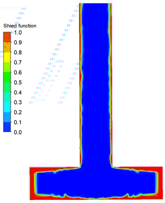
Figure 3.
The division of the numerical simulation domain by the hybrid model (blue, LES; red, RANS).
In this work, the PISO method was used for the pressure–velocity coupling. Gradient was discretized using the least square cell-based method. Pressure was discretized by second-order discretization. The bounded central differencing method was used to discretize the momentum. Time was integrated using the bounded second-order implicit method, and the discretization of other physical quantities was accomplished by the second-order upwind method. The Courant–Friedrichs–Lewy number was kept at 0.1, and the residuals of the iterations in each time step converged to 10−5.
3. Results and Discussion
3.1. Simulation Validation
In an MIVM, fluid can be regarded as swirling flows around the central axis, and then it flows out of the mixing chamber vertically, and so the validation of our simulation could be mainly based on the axial and tangential velocities, respectively. Therefore, we compared the fluid velocity obtained by the SDES simulation with a PIV experiment [16] to validate the simulation.
Figure 4 shows the axial and tangential velocities at the measurement plane shown in Figure 1b. It can be seen that for the axial velocity, when there were 1.2 million and 2.4 million grids, the relative deviations in the peak values with the experimental results were 16.0% and 16.3%, respectively, and for the tangential velocity, the relative deviations were 2.1% and 0.8%. Further, we could observe a clear grid dependence according to the result from the case with 0.6 million grids. When the number of grids increased from 1.2 million to 2.4 million, the relative deviations fluctuated within 2%, and it could be regarded that grid-independence was achieved.
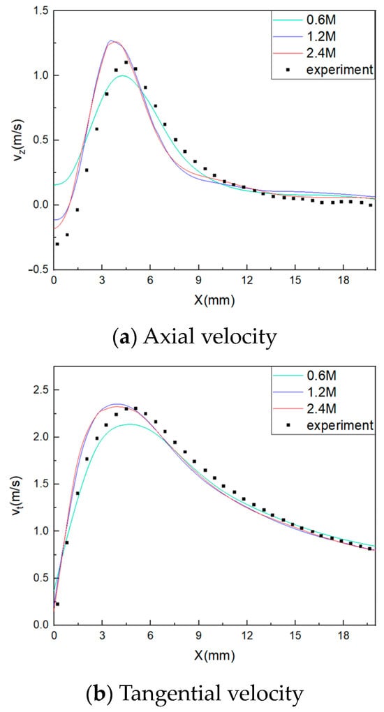
Figure 4.
Comparison of the velocities between the PIV experiment and the simulation.
Another important point in the judgement of grid validity is the fluid velocity near the center of a mixing chamber because the backmixing near there is targeted. In the case of 0.6 million grids, there was a positive velocity near the central axis of the mixing chamber, which was surely untrue compared with the result from the PIV. However, as shown in Figure 4a, in the case of 2.4 million grids, the velocity shown was negative, which was the closest among the three cases, while the relative deviation from the case of 1.2 million grids was 18.8% higher than that in this case. Therefore, in this work, the case with 2.4 million grids was applied.
3.2. Residence Time of Fluid
In evaluating the backflow behavior in the mixer, residence time distribution (RTD) is an effective method. By observing RTD curves, it is possible to judge the degree of backflow and the existence of short-circuit flows, channel flows or dead zones in a mixer. In this work, the single-inlet pulse method was used, and the concentration of the tracer was monitored at the outlet of the mixer while the concentration of the tracer was dimensionless by the volume ratio. The RTD curves of all ten cases are shown in Figure 5.
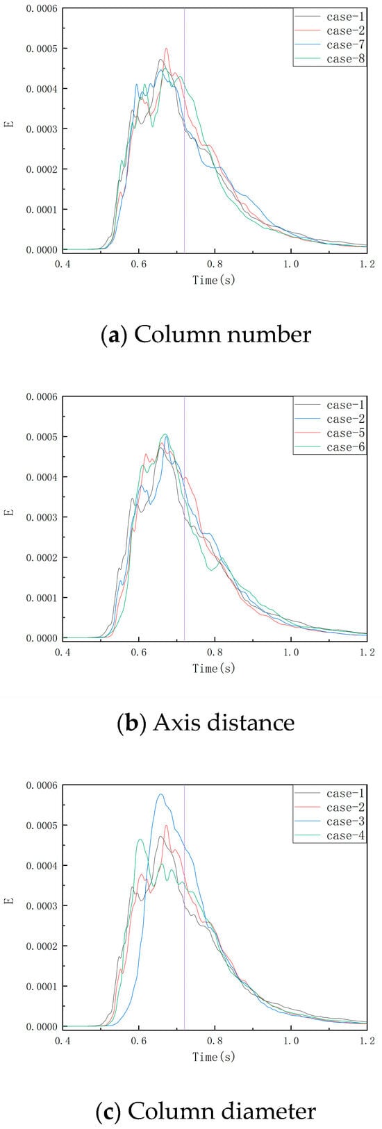
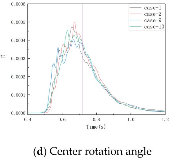
Figure 5.
The residence time distribution curves for the four groups of variables. The vertical lines indicate the average residence times.
According to the curves in Figure 5, it can be found that the change in the column diameter had a greater influence on the RTD curves compared with the other three variables.
Under the present operating condition, the average residence time of the fluid in the present MIVM was approximately 0.72 s, and this average time is represented by the vertical lines in Figure 5. By analyzing the RTD curve for case 1, it can be seen there were several problems in the scaled-up mixer, as follows:
- (1)
- There were multiple peaks appearing earlier than the average residence time, indicating that there may have been multiple short-circuit flows.
- (2)
- After the appearance of the maximum concentration on the RTD curve, the descending curve was not smooth, which showed that there may have been backflow.
- (3)
- There was an obvious tailing on the curve, which indicated the existence of backmixing in the mixer.
Generally speaking, short-circuit flow refers to the part that bypasses the main flow and flows out of a mixer. This situation is caused by defects in the geometry of a mixer. When analyzing the RTD curves in Figure 5, it can be found that the main peaks were obvious and each curve had only one main peak, which proved that there was no fully independent flow in the MIVM. Therefore, the cause of the multiple peaks was more likely to be channeling.
Interestingly, the causes of problem (1) and problem (2) mentioned above are partly the same. Figure 6 shows the mean velocity distribution on the middle cross-section of the MIVM, and it can be seen that a negative axial velocity region appeared in the very center of the mixing chamber (Figure 6a). This figure shows the existence of strong axial backflow in the MIVM. In the backflow region, the reverse flow would lead to an increase in the difference between the positive and negative flows, resulting in the early appearance of a main peak. Moreover, the fluid dispersion between the positive and negative flows would result in channeling in the mixer, which is shown as the multiple peaks on the RTD curves. As a comparison, in Figure 6b, the negative velocity region almost disappeared and the near-wall channel flows became weak.
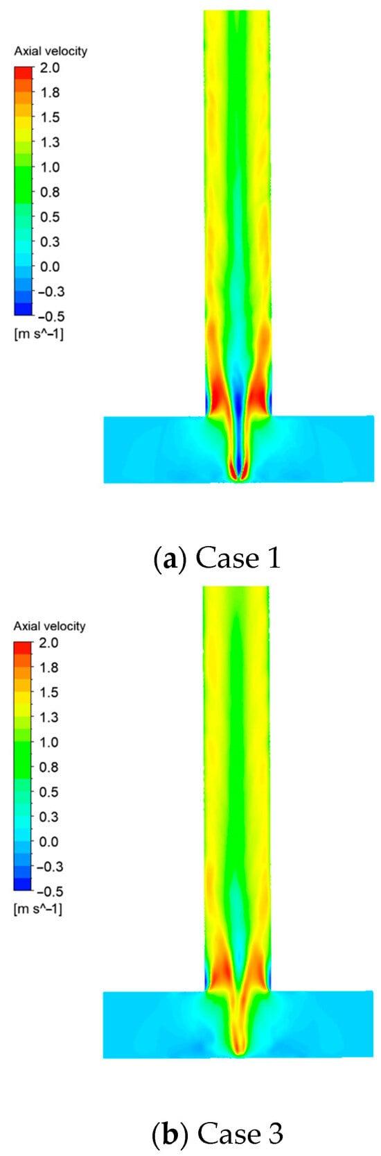
Figure 6.
Mean axial velocity distribution in the MIVM.
The coefficient of variation (COV), which is the ratio of the standard deviation to the mean, can be used to quantitively represent the uniformity of a velocity distribution. Here, we sampled the COV of the axial velocity on the cross-section along the outlet pipe of the mixer according to the vertical height, as shown in Figure 7. An apparent difference can be seen for those two curves, and the uniformities of the axial velocities on the sampling sections improved after the columns were installed in the mixing chamber, especially near the center.
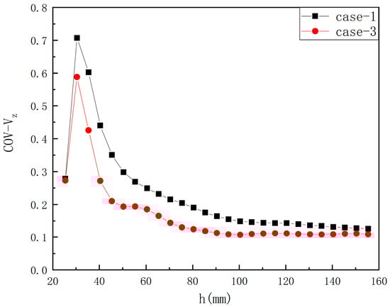
Figure 7.
Coefficient of variation of the axial velocity in the outlet pipe.
From the RTD curve for case 3, it can be seen that the disturbance generated by the columns showed three positive effects on the residence time of the fluid in the MIVM compared with the curve for case 1. These effects were:
- (1)
- The peak of the RTD curve appeared later and was closer to the average residence time.
- (2)
- The RTD curve ascended and descended more rapidly near the peak.
- (3)
- On RTD curve, the multi-peak phenomenon was almost eliminated.
Considering the RTD curves in Figure 5c and the axial velocity distribution in Figure 6b, it is clear that the disturbance generated by the columns would significantly weaken the backmixing in the outlet pipe.
Taking the least square fitting curve of the RTD curve as the base line, if the data deviated from the base line value by more than 20%, it could be regarded as a peak. Here, we counted the number of peaks to evaluate the channeling, as shown in Table 3.
Table 3.
Number of peaks on the RTD curves in the MIVM.
The solution in case 3 could basically solve the channeling problem. However, it can be seen from Table 3 that not all the cases with columns could solve the channeling problem in the mixer, and sometimes it was even worse. The reason may have been that a small amount of low-intensity wake vortexes was not enough to break the channel flows, but it separated one channel flow into more flows.
3.3. Tanks-in-Series Model
The tanks-in-series model can be used to quantitatively evaluate the degree of backmixing in the optimization of a reactor. A certain number of perfectly mixed flow reactors in series is used to be equivalent to non-ideal reactors. The larger the number of reactors, the more approximate it is to the plug flow reactor. As for the performance of an MIVM, a lower backflow or backmixing can lead to a narrower and more controllable particle size distribution.
Combining the results in Table 3 and Table 4, it could be seen that case 3 was the best solution for improving the flow in the MIVM. The number of equivalent mixers in case 3 was 49.6, which was 155% of that in case 1. In other words, while solving the channeling problem, case 3 greatly weakened the degree of backmixing.
Table 4.
RTD characteristic of the MIVM.
However, it should also be noted that not all the cases with columns could greatly improve the performance of the MIVM. For example, among the four groups of variables, only the axis distance and column diameter showed regularity. That is, as the diameter increased and the axis distance decreased, the number of equivalent mixers increased. However, the influences of the column number and rotation angle on the result were nearly random or undetermined. So, we drew the streamlines of the fluid on the measurement plane, as shown in Figure 8. In case 2, the wake vortexes behind the columns made the streamlines irregular, but the streamlines still showed a tendency to merge locally. In case 3, when the column diameter increased, the wake vortexes became stronger, and the streamlines did not tend to merge. Therefore, it could be supposed that the vortexes behind the columns weakened the degree of backmixing by re-separating the fluid that had converged under the rotating action.
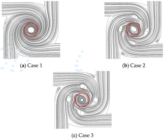
Figure 8.
Streamlines on the measurement plane. The red circles are the outlines of the outlet pipes.
By comparing the simulation results of the influence of the variables (the column number, diameter, etc.) on the mixer, the column diameter showed the greatest influence on the backmixing, which was the same as that shown in the RTD curves.
A vortex, which can be identified by the Q criterion [31], plays an important role in mixing in an MIVM. The Q criterion is based on the quadratic invariant of the velocity gradient tensor, as follows:
where the symmetric tensor Sij and antisymmetric tensor Ωij in the velocity gradient tensor are determined as follows:
when the Q value is greater than zero, it means that the rotation effect of the position in the flow field is stronger than the extension, and so the iso-surface of Q can be used to characterize the vortex structure of the flow field.
With columns, as shown in Figure 9b, many vortexes are generated around the columns and then flow with the main stream out of a mixer. Due to their existence, the continuity of the vortexes becomes poor near the center of the outlet pipe, where it is only the area with backflow. In case 3, the fluid not only rotated but also exhibited overall homogeneity, which created a turbulent flow with a partly laminar flow, such as that in the work of Kunhen et al. [32]. For example, they used vortexes to ‘lift up’ a low-velocity fluid from the wall and transported it towards the center to obtain a laminar flow. In this work, we dispersed the rotating fluid in the center to the wall to reach a similar result.
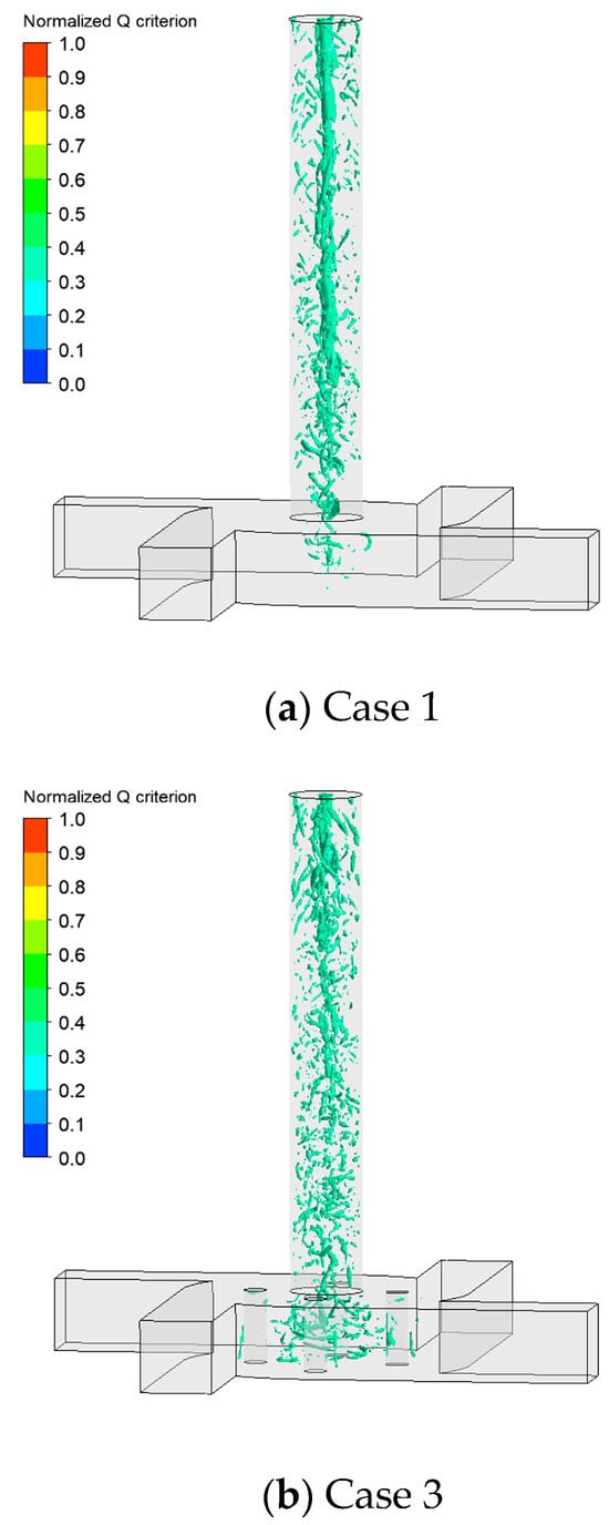
Figure 9.
Iso-surface of the normalized Q criterion in the MIVM.
In the MIVM, the fluid converged to the center of the mixing chamber from the four directions, and then it rotated out of the outlet. The closer to the center of the mixing chamber, the greater the angular velocity and the stronger the rotation, which led to an increase in the Q value. The rotation of the streams produced a centrifugal effect, and a large amount of liquid ran spiral against the pipe wall. As long as the center of an outlet pipe cannot hold the fluid, there will be a low-pressure area. Then, the surrounding fluid will swarm into the low-pressure area, and the backflow will form. The reason for backflow is nonuniform pressure distribution. Therefore, the role of the vortexes is mainly to make the kinetic energy of a fluid more evenly distributed in the center of a mixing chamber, avoiding the emergence of low-pressure areas, which are caused by the local excessive rotation of the fluid.
3.4. Turbulent Energy Dissipation
The rapid mixing in the MIVM was achieved by a high turbulent energy dissipation near the outlet of the mixing chamber. In order to explain whether the addition of columns would affect the performance of the mixer, we drew the contours of turbulent energy dissipation on the cross-section, as shown in Figure 10. It was clear that the position of the high energy dissipation area was unchanged, even when columns existed. However, the intensity was reduced. We sampled the energy dissipation rate of the fluid along the height of the outlet pipe, and we plotted the average energy dissipation rate and its coefficient of variation, as shown in Figure 11.
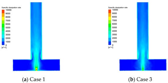
Figure 10.
Contours of the turbulent energy dissipation rate in the MIVM.
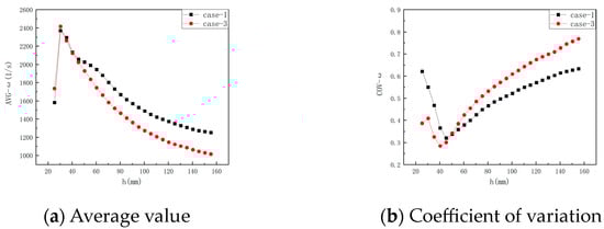
Figure 11.
Distribution of the turbulent energy dissipation rate in the outlet pipe.
As can be seen in Figure 11, after setting up columns in the mixing chamber, we successfully weakened the backflow, but the energy dissipation rate in the outlet pipe was also reduced, and so was the uniformity. Actually, as a part of the energy input by the streams was consumed on the vortex street, the energy for enhancing the mixing was certainly reduced. Therefore, when applying the columns to weaken the backflow or backmixing in an MIVM, the additional energy loss should be considered.
4. Conclusions
In the scaled-up MIVM, the SDES model could be used to accurately describe the rotating shear flow by means of a hybrid RANS–LES model. To solve the problem of axial backmixing and inspired by the idea of enhanced mixing by the Karman vortex street, we added columns in the mixing chamber and evaluated the performance of the mixer using a tanks-in-series model.
It was found that the existence of the columns had a significant effect on weakening the backmixing, and the diameter of the column was the most significant factor. As the main evaluation index, the number of equivalent mixers increased by 55%, and the peak number of the residence time distribution curve was reduced from four to one. After analyzing the vortexes in the mixer, we found that the center of the swirl coincided with the backmixing area, which meant that the centrifugal force caused by the swirling had a negative effect on the flow. The vortexes generated by the columns changed the structure of the swirling flow, avoiding local excessive rotation of the fluid, thereby weakening the backflow in the outlet pipe. It should be noted that there was extra energy loss in the improved MIVM compared with the original one, but the degree was acceptable.
All in all, this paper proposes a novel idea to weaken backmixing in a scaled-up MIVM using wake vortexes. This idea can be a useful guide for the design of MIVMs if scaling-up is required.
Author Contributions
Conceptualization, Z.L.; Writing—original draft, H.P.; Writing—review & editing, Z.C.; Supervision, Z.G. All authors have read and agreed to the published version of the manuscript.
Funding
The authors were supported by the National Natural Science Foundation of China (no. 21676007 and no. 22078008) and the Fundamental Research Funds for the Central Universities (XK1802-1).
Data Availability Statement
Data are contained within the article.
Acknowledgments
The authors would also like to acknowledge the Center for Fluid Mixing and Reactor Engineering of Beijing University of Chemical Technology for providing access to the computer cluster.
Conflicts of Interest
The authors declare no conflict of interest.
Abbreviations
| Nomenclature | |
| k | Turbulent kinetic energy, m2·s−2 |
| ω | Specific energy dissipation rate, s−1 |
| Win | Width of the inlet, mm |
| Lin | Length of the inlet, mm |
| Dout | Diameter of the outlet pipe, mm |
| Lin | Length of the outlet pipe, mm |
| Hmix | Height of the mixing chamber, mm |
| Dmix | Diameter of the mixing chamber, mm |
| Re | Reynolds number |
| N | Number of columns |
| ΔL | Axis distance between the center of column and center of mixer, mm |
| φ | Diameter of the column, mm |
| θ | Angle of rotation around the center, ° |
| μt | Turbulent eddy viscosity, kg·m−1·s−1 |
| Pk | Generating term of the turbulent kinetic energy, kg·m−1·s−3 |
| ρ | Fluid density, kg·m−3 |
| U | Fluid velocity, m·s−1 |
| μ | Fluid viscosity, kg·m−1·s−1 |
| hmax | Maximum edge length of the grid, mm |
| l | Length scale of the turbulent model, mm |
| S | Magnitude of the strain rate tensor, s−1 |
| Ω | Magnitude of the vorticity tensor, s−1 |
| dw | Distance from the grid to the nearest wall, mm |
| V | Volume of the cell, mm3 |
| vz | Axial velocity, m·s−1 |
| vt | Tangential velocity, m·s−1 |
| Q | Q criterion, s−2 |
| uij | ∂ui/∂xj, s−1 |
| uji | ∂uj/∂xi, s−1 |
| Abbreviations | |
| FNP | Flash nanoprecipitation |
| CIJ | Confined impinging jet |
| MIVM | Multi-inlet vortex mixer |
| CFD | Computational fluid dynamics |
| PIV | Particle image velocimetry |
| PLIF | Planar laser-induced fluorescence |
| SDES | Shielded detached eddy simulation |
| SST | Shear-stress transport |
| RANS | Reynolds-averaged Navier–Stokes |
| LES | Large-eddy simulation |
| DDES | Delayed detached eddy simulation |
| DES | Detached eddy simulation |
| RTD | Residence time distribution |
| COV | Coefficient of variation |
References
- Zhao, Y.B.; Qiu, Z.M.; Huang, J.Y. Preparation and analysis of Fe3O4 magnetic nanoparticles used as targeted-drug carriers. Chin. J. Chem. Eng. 2008, 16, 451–455. [Google Scholar] [CrossRef]
- Wicki, A.; Witzigmann, D.; Balasubramanian, V.; Huwyler, J. Nanomedicine in cancer therapy: Challenges, opportunities, and clinical applications. J. Control. Release 2015, 200, 138–157. [Google Scholar] [CrossRef] [PubMed]
- Xiao, S.Y.; Tang, Y.F.; Lv, Z.; Lin, Y.M.; Chen, L. Nanomedicine—Advantages for their use in rheumatoid arthritis theranostics. J. Control. Release 2019, 316, 302–316. [Google Scholar] [CrossRef]
- Wilson, B.; Geetha, K.M. Neurotherapeutic applications of nanomedicine for treating Alzheimer’s disease. J. Control. Release 2020, 325, 25–37. [Google Scholar] [CrossRef]
- Huo, M.F.; Wang, L.Y.; Chen, Y.; Shi, J.L. Nanomaterials/microorganism-integrated microbiotic nanomedicine. Nano Today 2020, 32, 100854. [Google Scholar] [CrossRef]
- Johnson, B.K.; Prud’homme, R.K. Flash nanoprecipitation of organic actives and block copolymers using a confined impinging jets mixer. Aust. J. Chem. 2003, 56, 1021–1024. [Google Scholar] [CrossRef]
- Valente, I.; Stella, B.; Marchisio, D.L.; Dosio, F.; Barresi, A.A. Production of PEGylated nanocapsules through solvent displacement in confined impinging jet mixers. J. Pharm. Sci. 2012, 101, 2490–2501. [Google Scholar] [CrossRef]
- Tao, J.S.; Chow, S.F.; Zheng, Y. Application of flash nanoprecipitation to fabricate poorly water-soluble drug nanoparticles. Acta Pharm. Sin. B 2019, 9, 4–18. [Google Scholar] [CrossRef] [PubMed]
- Shi, L.; Shan, J.N.; Ju, Y.G.; Aikens, P.; Prud’homme, R.K. Nanoparticles as delivery vehicles for sunscreen agents. Colloids Surf. A Physicochem. Eng. Asp. 2012, 396, 122–129. [Google Scholar] [CrossRef]
- Liu, Y.; Olsen, M.G.; Fox, R.O. Turbulence in a microscale planar confined impinging-jets reactor. Lab Chip 2009, 9, 1110–1118. [Google Scholar] [CrossRef]
- Liu, Y.; Cheng, C.Y.; Liu, Y.; Prud’homme, R.K.; Fox, R.O. Mixing in a multi-inlet vortex mixer (MIVM) for flash nano-precipitation. Chem. Eng. Sci. 2008, 63, 2829–2842. [Google Scholar] [CrossRef]
- D’Addio, S.M.; Prud’homme, R.K. Controlling drug nanoparticle formation by rapid precipitation. Adv. Drug Deliv. Rev. 2011, 63, 417–426. [Google Scholar] [CrossRef]
- Akbulut, M.; Ginart, P.; Gindy, M.E.; Theriault, C.; Chin, K.H.; Soboyejo, W.; Prud’homme, R.K. Generic method of preparing multifunctional fluorescent nanoparticles using flash nanoprecipitation. Adv. Funct. Mater. 2009, 19, 718–725. [Google Scholar] [CrossRef]
- Kumar, V.; Adamson, D.H.; Prud’homme, R.K. Fluorescent polymeric nanoparticles: Aggregation and phase behavior of pyrene and amphotericin B molecules in nanoparticle cores. Small 2010, 6, 2907–2914. [Google Scholar] [CrossRef] [PubMed]
- Shen, H.; Hong, S.; Prud’homme, R.K.; Liu, Y. Self-assembling process of flash nanoprecipitation in a multi-inlet vortex mixer to produce drug-loaded polymeric nanoparticles. J. Nanoparticle Res. 2011, 13, 4109–4120. [Google Scholar] [CrossRef]
- Liu, Z.P.; Hill, J.C.; Fox, R.O.; Olsen, M.G. Investigation of turbulent mixing in a macro-scale multi-inlet vortex nanoprecipitation reactor by stereoscopic-PIV. In Proceedings of the ASME 2014 4th Joint US-European Fluids Engineering Division Summer Meeting, Chicago, IL, USA, 11–15 July 2014. [Google Scholar]
- Liu, Z.P.; Ramezani, M.; Fox, R.O.; Hill, J.C.; Olsen, M.G. Flow characteristics in a scaled-up multi-inlet vortex nanoprecipitation reactor. Ind. Eng. Chem. Res. 2015, 54, 4512–4525. [Google Scholar] [CrossRef]
- Liu, Z.P.; Passalacqua, A.; Olsen, M.G.; Fox, R.O.; Hill, J.C. Dynamic delayed detached eddy simulation of a multi-inlet vortex reactor. AIChE J. 2016, 62, 2570–2578. [Google Scholar] [CrossRef]
- Liu, Z.P.; Hitimana, E.; Olsen, M.G.; Hill, J.C.; Fox, R.O. Turbulent mixing in the confined swirling flow of a multi-inlet vortex reactor. AIChE J. 2017, 63, 2409–2419. [Google Scholar] [CrossRef]
- Cheng, J.C.; Olsen, M.G.; Fox, R.O. A microscale multi-inlet vortex nanoprecipitation reactor: Turbulence measurement and simulation. Appl. Phys. Lett. 2009, 94, 204104. [Google Scholar] [CrossRef]
- Leon, M.A.; Nijhuis, T.A.; Schaaf, J.V.D.; Schouten, J.C. Residence time distribution and reaction rate in the horizontal rotating foam stirrer reactor. Chem. Eng. Sci. 2014, 117, 8–17. [Google Scholar] [CrossRef]
- Bhutto, R.A.; Bhutto, N.H.; Iqbal, S.; Manoharadas, S.; Yi, J.; Fan, Y.T. Polyelectrolyte nanocomplex from sodium caseinate and chitosan as potential vehicles for oil encapsulation by flash nanoprecipitation. Food Hydrocolloid 2024, 150, 109666. [Google Scholar] [CrossRef]
- Lass, H.U.; Mohrholz, V.; Knoll, M.; Prandke, H. Enhanced mixing downstream of a pile in an estuarine flow. J. Mar. Syst. 2008, 74, 505–527. [Google Scholar] [CrossRef]
- Dundi, T.M.; Raju, V.R.K.; Chandramohan, V.P. Characterization of mixing in an optimized designed T–T mixer with cylindrical elements. Chin. J. Chem. Eng. 2019, 27, 2337–2351. [Google Scholar] [CrossRef]
- Li, L.; Xu, W.X.; Tan, Y.F.; Yang, Y.S.; Yang, J.G.; Tan, D.P. Fluid-induced vibration evolution mechanism of multiphase free sink vortex and the multi-source vibration sensing method. Mech. Syst. Signal Process. 2023, 189, 110058. [Google Scholar] [CrossRef]
- Blevins, R.D.; Scanlan, R.H. Flow-induced vibration. J. Mech. Des. N. Y. 1977, 44, 802. [Google Scholar] [CrossRef]
- Travin, A.; Shur, M.; Strelets, M.; Spalart, P. Detached-eddy simulations past a circular cylinder. Flow Turbul. Combust. 1999, 63, 293–313. [Google Scholar] [CrossRef]
- Zhao, W.W.; Wan, D.C.; Sun, R. Detached-eddy simulation of flows over a circular cylinder at high Reynolds number. In Proceedings of the 26th International Ocean and Polar Engineering Conference, Rhodes, Greece, 26 June–1 July 2016. [Google Scholar]
- ANSYS Inc. ANSYS Fluent Theory Guide; ANSYS Inc.: Canonsburg, PA, USA, 2017. [Google Scholar]
- Gritskevich, M.S.; Garbaruk, A.V.; Schutze, J.; Menter, F.R. Development of DDES and IDDES formulations for the k-ω shear stress transport model. Flow Turbul. Combust. 2012, 88, 431–449. [Google Scholar] [CrossRef]
- Jeong, J.; Hussain, F. On the identification of a vortex. J. Fluid Mech. 1995, 285, 69–94. [Google Scholar] [CrossRef]
- Kuhnen, J.; Song, B.F.; Scarselli, D.; Budanur, N.B.; Riedl, M.; Willis, A.P.; Avila, M.; Hof, B. Destabilizing turbulence in pipe flow. Nat. Phys. 2018, 14, 386–390. [Google Scholar] [CrossRef]
Disclaimer/Publisher’s Note: The statements, opinions and data contained in all publications are solely those of the individual author(s) and contributor(s) and not of MDPI and/or the editor(s). MDPI and/or the editor(s) disclaim responsibility for any injury to people or property resulting from any ideas, methods, instructions or products referred to in the content. |
© 2024 by the authors. Licensee MDPI, Basel, Switzerland. This article is an open access article distributed under the terms and conditions of the Creative Commons Attribution (CC BY) license (https://creativecommons.org/licenses/by/4.0/).