Abstract
Effective fault diagnosis for diaphragm pumps is crucial. This paper proposes a diaphragm pump fault diagnosis method based on deep learning and multi-source information fusion (DMF). The time-domain features, frequency-domain features, and modulation features are extracted from the vibration signals from eight different positions. After feature enhancement and data preprocessing, the features are input into auto encoders (AE), convolutional neural networks (CNN), and support vector machines (SVM) to obtain the diagnostic results. The results indicate that the DMF method achieves a fault diagnosis accuracy of 99.98%, which is on average 9.09% higher than using a single diagnostic model. The demodulation method is more suitable for vibration signal feature extraction of the diaphragm pump, while the CNN is more suitable for identification of diaphragm pump faults. Specifically, it outperformed the sampling point 1-DPCA-AE model by 13.98% and the sampling point 4-DPCA-SVM model by 8.98%.
1. Introduction
Diaphragm pumps are critical equipment widely used in the chemical, pharmaceutical, and food industries, and their reliable operation is crucial for production safety and efficiency [1]. However, due to the complexity of their working environment and the characteristics of the equipment itself, diaphragm pumps are prone to failures [2]. Failure to promptly detect and diagnose these faults may lead to severe economic losses or even safety accidents [3]. Therefore, effective fault diagnosis and health monitoring of diaphragm pumps are key to enhancing their reliability and safety [4].
There are various types of failures in diaphragm pumps, including, but not limited to, diaphragm rupture, inadequate lubrication, and malfunctioning check valves [5]. The occurrence of these failures is often associated with multiple factors such as material fatigue, improper operation, and inadequate maintenance [6]. To accurately diagnose the types and causes of diaphragm pump failures, researchers have employed various methods, including acoustic diagnosis, vibration analysis, and pressure monitoring [7]. While each of these methods has its advantages and disadvantages, they all to some extent increase the complexity and cost of fault diagnosis [8]. With the rapid development of information technology and artificial intelligence, data-driven fault diagnosis techniques have garnered significant attention, providing novel perspectives and methodologies for diaphragm pump fault diagnosis [9]. Data-driven fault diagnosis techniques primarily rely on a large volume of operational data and advanced data processing technologies [10]. By collecting and analyzing the data during the operation of diaphragm pumps, it is possible to effectively identify abnormal patterns, thereby achieving the early warning and accurate diagnosis of faults [11]. This process typically involves data collection, feature extraction, pattern recognition, and fault classification. Data collection is fundamental and requires real-time monitoring of the pump’s operating status using various sensors, such as temperature, pressure, and flow rate [12]. Feature extraction is critical and involves extracting useful information for fault diagnosis from a large amount of raw data [13]. Pattern recognition and fault classification are essential, requiring the application of deep learning algorithms to accurately discriminate and classify fault types based on the extracted features [14]. In recent years, deep learning technology has made significant advancements in pattern recognition and data analysis, demonstrating strong performance, particularly in fields such as image recognition, speech processing, and natural language processing. However, its application in industrial equipment fault diagnosis, especially in diaphragm pump fault diagnosis, is still in its early stages. Furthermore, despite the enormous potential shown by data-driven fault diagnosis techniques in theory and practice, they still face some challenges in actual applications [15]. First, the complex and constantly changing operating environment in which diaphragm pumps operate makes them susceptible to interference from external factors during data collection, affecting the accuracy and reliability of the data [16]. Second, the complex and diverse failure modes of diaphragm pumps demand that fault diagnosis systems be highly flexible, adaptive, and capable of accurately identifying and handling various abnormal situations [17]. Additionally, efficient feature extraction and advanced data processing technologies are crucial for the accuracy of fault diagnosis. However, in industrial systems, due to the complexity and diversity of fault signals, it is often a challenge to cover all potential fault scenarios and to accurately diagnose specific fault types with a single data source and data processing method [18].
By comprehensively considering the data from multiple sensors and various data processing methods, it is possible to more effectively identify and isolate faults, and even issue early warnings in the initial stages of a fault, thereby reducing system downtime and maintenance costs [19]. Additionally, the fusion of multisource information also aids in identifying and eliminating false alarms, enhancing the stability and reliability of fault diagnostic systems [20]. In practical applications, this fusion approach not only improves the accuracy of fault diagnosis but also provides richer information for maintenance decision-making, significantly enhancing the overall operational efficiency and safety of the equipment [21]. Researchers have conducted a series of studies on fault diagnosis using multisource information fusion. Xu W et al. [19] have proposed a multi-model decision fusion method for rolling bearing fault detection, utilizing a deep convolutional neural network (DCNN) and an improved Dempster–Shafer theory (IDST). The introduction of a fuzzy consistency matrix overcomes the limitations of the original evidence theory method in handling the fusion of highly conflicting evidence. They also introduced a multi-sensor time-series signal RUL prediction method based on a DLSTM network. Wu J et al. [22] adjusted the network structure and parameters of the DLSTM model by integrating multiple sensor-monitoring signals using grid search and adaptive matrix estimation algorithms. They validated the performance of the DLSTM model using two different turbofan engine datasets. Zhao X et al. [23] have proposed a fault diagnosis method based on multi-sensor signals and principal component analysis (PCA). By analyzing the correlation of multi-sensor signals, they derived simplified fault diagnosis statistical indicators using PCA, enabling the online monitoring of the FCS operating status and diagnosis of sensor and system-level faults. This study combined original time-domain signals, spectra, and demodulated spectra, inputting them into a convolutional neural network, support vector machine, and auto encoder. By employing decision-level fusion through DS evidence theory, the comprehensive identification of diaphragm pump faults was achieved.
In summary, to enhance the diagnostic accuracy of diaphragm pumps, this paper presents a method that integrates deep learning with multiple sources of information. In Section 2, the paper introduces signal demodulation methods, deep learning network models, and DS evidence theory. Section 3 covers the experimental setup, while Section 4 presents the diagnostic results of the proposed method and conducts a comparative analysis with a single diagnostic model. Finally, Section 5 concludes the paper.
2. Basic Theory
This section presents a diagnostic model for diaphragm pump failures, one which utilizes deep learning techniques and integrates the multi-source information fusion of vibration signals. The model framework, illustrated in Figure 1, comprises four main components: multi-source data collection, multi-source feature extraction, training and optimization of deep learning models, and decision-level multimodal fusion.
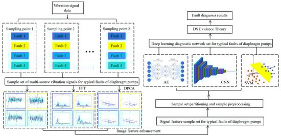
Figure 1.
DMF model schematic diagram.
First, vibration signals from multiple sampling points of the diaphragm pump are collected throughout its entire lifecycle to form a comprehensive lifecycle sample set. Samples are selected based on equipment maintenance records to create a fault sample set. Then, time-domain features, frequency-domain features, and modulation features of each signal segment are extracted to generate image samples.
Data augmentation is achieved through the stitching of these image samples. Subsequently, the image samples are inputted into auto encoders (AE), convolutional neural networks (CNN), and support vector machines (SVM) for image sample classification and recognition, thereby establishing various fault diagnostic models. Model validation and performance optimization are then carried out. Lastly, to improve diagnostic accuracy and robustness, DS evidence theory is employed to integrate multiple different deep learning models. The synthesis of evidence from the various models results in a unified judgment, enhancing the emphasis on the management of erroneous samples in single diagnostic models and ultimately improving overall diagnostic model precision.
2.1. Signal Demodulation Algorithm DPCA
Different types of faults may manifest as different frequency components in the vibration signal, making signal demodulation useful for extracting such information from complex environments. DPCA is an efficient signal demodulation algorithm based on time–frequency analysis and principal component analysis. Firstly, the original signal is subjected to time–frequency analysis using a Hanning window. Next, a time–frequency distribution matrix is obtained by solving the time–frequency distribution function. Subsequently, the matrix is subjected to covariance operation, followed by principal component analysis. Finally, a fast Fourier transform is applied for time–frequency domain transformation. The key to this algorithm lies in the extraction of signal principal components, with the following steps:
- (a)
- Time–frequency distribution matrix
The time–frequency distribution function obtained through Equation (1) and STFT can be used to obtain the signal’s amplitude spectral density function , where is the Fourier transform length of the window function.
Extracting time–frequency distribution matrices facilitates the study of signal variations in time and frequency domains. These matrices depict the energy distribution of signals in both time and frequency domains, aiding in the identification of transient phenomena, frequency components, and their temporal evolution. The calculation of the time–frequency distribution matrix is represented by Equation (2):
- (b)
- Covariance matrix
The covariance matrix can be used to extract correlation information between signals. By calculating the covariance between different signals, one can understand their linear correlation or the degree of correlation over time. The time–frequency distribution matrix is obtained by using the covariance function to obtain the corresponding covariance matrix, as shown in Equation (3):
- (c)
- Eigenvalue decomposition
We used the eigenvalue decomposition method to obtain the eigenvalues and eigenvectors of the matrix, as shown in Equation (4):
In the equation, represents the feature decomposition operator, is a diagonal matrix composed of eigenvalues , and is a matrix composed of eigenvectors corresponding to eigenvalues.
- (d)
- Principal component reconstruction
Using differential universal selection to obtain the eigenvectors corresponding to the first k-th order eigenvalues, the selection rule is shown in Equation (5):
where k represents the number of principal components and represents the positive difference between adjacent values. The selected feature vectors are reconstructed to obtain the principal component signal, as shown in Equation (6):
represents the periodic principal component of the signal, which can extract feature modulation frequency through frequency analysis.
2.2. Deep Learning Models
The extracted feature samples are separately fed into AE, CNN, and SVM to learn image features using training data. This process is then utilized to predict classifications on new samples, resulting in independent fault diagnosis models.
2.2.1. Auto Encoder (AE)
AE is a neural network used for learning the efficient representation of data. An auto encoder is a specialized neural network designed to compress input data into a meaningful representation, and then reconstruct it to closely resemble the original input. It usually consists of an encoder and a decoder. The encoder maps the input data to a hidden layer representation, as shown in Equation (7), while the decoder maps this representation back to the original input space, as shown in Equation (8).
Among these, is the input, is the hidden layer representation, and are the activation functions, , , and and are the weights and biases of the encoder and decoder, respectively. The training goal of auto encoder is to minimize the difference between and .
2.2.2. CNN
A convolutional neural network (CNN) typically comprises convolutional layers, pooling layers, and fully connected layers. Convolution involves sliding a small window (convolution kernel) across input data, performing element-wise multiplication and sum operations to generate an output feature map. As shown in Equation (9), the pooling layer reduces the spatial dimensions of the feature map. Fully connected layers map the extracted features to output categories.
where is the feature map of layer , is the input image, is the convolution kernel, and is the bias.
VGG16, a deep CNN, features 13 convolutional layers, 5 pooling layers, and 3 fully connected layers. Utilizing multiple 3 × 3 convolution kernels, VGG16 conducts convolution operations and employs rectified linear unit (ReLU) activation function after each convolution layer to enhance nonlinear feature expression.
2.2.3. SVM
Support vector machines (SVMs) are powerful supervised learning models commonly used for classification tasks, including image classification and recognition. SVMs aim to find the optimal hyperplane that maximally separates data points belonging to different classes in feature space. This hyperplane is determined by support vectors, which are the data points closest to the decision boundary. SVMs are particularly effective in high-dimensional spaces, making them well-suited for tasks like image classification where each pixel or feature contributes to a potentially large feature space.
SVMs can be extended to handle multi-class classification tasks using strategies like one-vs-one or one-vs-all classification. The decision function Equation (10) is shown as follows:
where is the weight vector, is the deviation, and is the input sample.
2.3. Model Evaluation Indicators
When evaluating deep learning classification models, performance is typically measured using the accuracy of the test set as the main indicator. Accuracy provides a straightforward indication of a model’s ability to correctly classify instances in the test data. However, relying solely on accuracy may obscure the model’s true performance, especially in the presence of class imbalances or varying error costs. Focusing exclusively on accuracy could result in biased model evaluations.
The F1 score, a widely used metric for evaluating the performance of multi-classification models, is calculated as the harmonic mean of model precision and recall. Therefore, F1 score can more comprehensively evaluate the performance of the model. The equation for calculating the F1 score is as follows:
Recall = (number of samples correctly predicted)/(number of samples correctly predicted + number of samples predicted as other categories but are actually of the same category).
Precision = (number of samples correctly predicted)/(number of samples correctly predicted + number of samples predicted as this category but are actually of other categories).
In this decision-making process, we first obtain the confusion matrix for each model on the test set, and then calculate their F1 scores. We choose the top nine models based on their F1 scores for the fusion process, aiming to create high-performing fused models. This method effectively filters out high-performing models from a large pool, providing a solid foundation for the final decision fusion.
2.4. DSET
In the context of multi-source information fusion, there are challenges in integrating information from different sensors or modes, with varying reliability and confidence. The DSET provides a mathematical framework for managing uncertain and imprecise information by assigning belief functions to different pieces of evidence. The core of DSET lies in addressing uncertainty and integrating multi-source information. The following is the basic process of DSET.
- (a)
- Identification framework
The set discrimination framework represents N identifiable objects related to through mutually exclusive categories. Its set expression is given by Equation (12).
If a function satisfies Equation (12), it is considered a probability distribution function on , with being the basic probability measure of A. represents the degree of trust in hypothesis set A based on the current context. The function of the probability distribution is to map any subset of to a number on
- (b)
- Trust distribution
The DS evidence theory describes the degree of trust in a hypothesis or subset using belief distribution. It uses belief and plausibility functions to indicate trust and distrust in a subset. Bel(A) represents the trust level in hypothesis set A in the current environment, calculated as the sum of the basic probabilities of all subsets of A, as shown in Equation (13), reflecting the overall trust in A.
In this context, represents the trust level of subset B, typically determined by the outputs of individual sensors or recognition models.
The likelihood function is also known as the irrefutable function or upper limit function. indicates the trust level in , or more specifically, the trust level in A being false; therefore, signifies the trust level in A being not false.
- (c)
- Synthesis rules
The unique aspect of DSET lies in its ability to integrate information from different sensors, models, or data sources. DS synthesis rules primarily compute new DS evidence by intersecting and uniting existing DS evidence. If m1 and m2 are two quality functions formed from information obtained from two different sources within the same recognition framework, then their orthogonality satisfies the following:
where K is the conflicting factor. When , the orthogonal sum m becomes a probability distribution function. When , there is no orthogonal sum m, and m1 and m2 are considered contradictory.
3. Experiments
3.1. Experimental Setup
To demonstrate the feasibility and effectiveness of a methodology, this study utilizes vibration signal data obtained from the DGMB580-9A diaphragm pump at Fusheng Aluminum Industry in Yuncheng City, Shanxi Province, manufactured by Shenyang Pump Industry in May 2014, for experimental validation. The equipment comprises a drive system, a transmission system, a pump head system, and a control system, represented in Figure 2 and Figure 3. Specifically, the drive system is composed of a motor and the connecting components responsible for providing power to the pump. The transmission system incorporates a gearbox and a camshaft, with the gearbox designed to adjust the output torque by reducing the motor speed. The pump head system is the primary system of the diaphragm pump, consisting of a diaphragm, pump chamber, valve, and pump body. Finally, the control system is principally governed by the controller, which serves to regulate and manage the operational functions of the pump. The code runs on a 64-bit Windows 10 operating system installed on a laptop with an Intel Core i5-12400 processor, Intel UHD Graphics 730, and 16 GB of RAM.
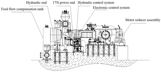
Figure 2.
Assembly diagram of DGMB580-9A diaphragm pump.
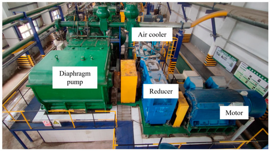
Figure 3.
Experimental setup diagram.
Eight vibration acceleration sensors were employed in this experiment to capture vibration signals from a diaphragm pump operating under typical fault conditions. The sampling time for each data collection was 3.2 s, and the sampling frequency was set at 5120 Hz. The pump’s vibrations reflect the internal mechanical motion and any issues related to transporting the media. The vibration at the motor drive end is typically associated with the motor’s load, bearing status, and connection between the motor and pump. Analyzing the vibration signal from the gearbox can identify problems such as gear wear, poor lubrication, and bearing faults. Therefore, the signal collection points were set on the pump body, motor drive end, and gearbox to capture these specific vibration signals. The specific signal collection points and directions are detailed in Table 1.

Table 1.
Vibration sensor layout table.
3.2. Fault Setting
This experiment investigated four common types of diaphragm pump failures, namely Fault 1: Lubrication Pump Failure (LPF); Fault 2: Check Valve Failure (CVF); Fault 3: Diaphragm Degradation (DD); and Fault 4: Gearbox Cooling Fan Fault (GCFF).
- (a)
- Lubrication Pump Failure
LPF is typically caused by internal pump wear, seal failure, or oil path blockage. This failure affects the pump’s flow rate and pressure stability. Unstable lubricating oil supply may accelerate internal pump wear and eventually lead to complete pump failure. Understanding the characteristics of LPF is crucial for predicting and preventing more severe mechanical damage.
- (b)
- Check Valve Failure
A malfunctioning check valve can cause internal components to wear out or become jammed, resulting in the valve’s inability to function properly. Valve failure can lead to unstable system pressure, impacting the efficiency of the entire pump. Investigating this issue is essential for ensuring system stability and preventing larger-scale equipment damage.
- (c)
- Diaphragm Degradation
Diaphragm failures typically result from material aging or mechanical stress, leading to diaphragm rupture or failure. Diaphragm damage may cause a decrease in pump efficiency and, in severe cases, internal leakage. Accurately diagnosing diaphragm failure is crucial for maintaining the pump’s normal operation and preventing liquid leakage.
- (d)
- Gearbox Cooling Fan Fault
The main causes of the failure of the speed reducer cooling fan are damaged fan blades, motor malfunction, or poor ventilation. Cooling fan failure can lead to overheating of the speed reducer, potentially impacting its performance and lifespan. Monitoring and diagnosing the cooling fan’s status are crucial for maintaining optimal working conditions of the speed reducer and extending equipment lifespan.
3.3. Data Processing
Each fault experiment collected 800 sets of signals under various operating conditions, with each set comprising 8 vibration signals from sensors and consisting of 16,384 data points. The signals were processed to generate time domain plots, frequency domain plots, and demodulated plots, forming feature images.
In this study, we grouped every four feature images into a 2 × 2 input unit to reduce data volume, enhance computational efficiency, and mitigate overfitting in deep learning models. After merging, there were 800 samples of single category feature images under each of the four fault conditions. These image data samples were input into AEs, CNNs, and SVMs to establish classification models. Due to variations in feature image acquisition methods, sensor placements, and deep learning models, a total of 72 models were generated. Each model was trained using 480 data samples, validated with 120 samples, and tested with the remaining 200 samples [24].
3.4. Parameter Settings
Due to the limited sample size of 480 in the training set, the key to setting the model parameters is to avoid overfitting and to learn effective feature representations from the limited data. Proper regularization and precise parameter selection are crucial in this process. Additionally, evaluating the model performance through cross-validation is important, as the characteristics of each dataset may vary.
The VGG16 model requires a large amount of data. To prevent overfitting, use of a small learning rate and data augmentation is recommended, while transfer learning can leverage features learned on a large dataset. Therefore, a batch size of 16 was chosen to fully utilize the data and maintain good generalization ability, and the learning rate was set to 0.001 to stabilize the training process.
The purpose of auto encoders is to learn efficient data representations. A moderate network complexity helps to extract features without causing overfitting. Cross-entropy, suitable for classification problems, is chosen as the loss function. Each layer has 128 neurons, with L1 and L2 regularization used to prevent the model from overfitting the training data and reduce overfitting.
On a limited dataset, the selection of kernel and parameter adjustment for SVM is particularly important to ensure that the model captures complex relationships between data without overfitting. A simple linear kernel is chosen for the kernel function. The C parameter controls the penalty for misclassified data points. A high C value imposes a larger penalty for misclassifications, leading the model to maximize correct classification of the training data and potentially causing overfitting. On the other hand, a low C value allows for greater tolerance of misclassification, making the model more generalizable, but it may also lead to underfitting. Through multiple experimental validations, the C value was set to 1.0.
4. Model Fusion and Discussion
4.1. Model Selection
The test dataset was input into 72 trained recognition models, resulting in 72 confusion matrices of classification results. Then, we calculated the F1 scores of these matrices and selected the nine models with the highest F1 scores. These selected models and their corresponding confusion matrices for the test dataset are summarized in Table 2 and shown in Figure 4, respectively.
Table 2.
Selected model table.
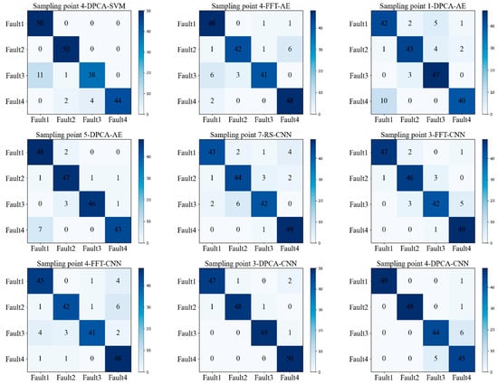
Figure 4.
Confusion matrix of test results.
4.2. Decision Fusion
In this study, the generalization capability of network models was harnessed to formulate the basic probability assignment (BPA) for the DSET. The accuracy derived from the test dataset served as evidence for decision-level fusion within the DSET. The basic belief assignment functions for each fault condition were calculated for the model obtained in Section 3.4 to obtain the local and global credibilities of the model, as shown in Table 3. The data in Table 3 were used as prior information to reallocate the basic belief assignment functions for each condition. The fault diagnosis results for multi-sensor fusion and a single model under the DSET were obtained based on the maximum membership principle. The outputs of the nine models were normalized and used as the BPA for the DSET, as shown in Table 4. Then, fusion was carried out using existing conditions according to Equation (15).
Table 3.
Classification credibility of the model.
Table 4.
BPA of the model.
4.3. Model Fusion Results and Comparative Analysis
With the addition of credible evidence in the fusion process, BPA continues to increase. Based on the method proposed in this paper, the final diagnostic accuracy reached 99.98%, surpassing the diagnostic accuracy of any single network model and averaging a 9.09% improvement over single diagnostic models. As indicated in Table 5, prior to fusion, the lowest accuracy among the nine models was 86.00% for model 3 (sampling point 1-DPCA-AE). Upon fusion with models 1, 4, 8, and 9 to form the DPCA model, the accuracy of model 3 increased by 13.53%. Similarly, upon fusion with models 2 and 4 to form the AE model, the accuracy of model 3 increased by 10.45%. Model 8 achieved the highest accuracy, at 97.00%. Upon fusion with the DPCA model, the accuracy of model 8 increased by 3.53%. When combined with the CNN model, the accuracy of model 8 increased by 3.52%. Clearly, the fusion of multi-source information leads to higher fault diagnostic accuracy, enabling more accurate identification of diaphragm pump failures.
Table 5.
Accuracy of fusion model.
In order to further compare the recognition characteristics of different diagnostic models, two sets of comparative experiments were established. Firstly, a comparison of the impact of different feature extraction methods on diagnostic accuracy under CNN neural network conditions. Secondly, after performing DPCA on the collected signals, a comparison of the impact of different deep learning networks on diagnostic accuracy. The comparison results are shown in Figure 5 and Figure 6. The DPCA method has higher diagnostic accuracy than the original signal and the FFT signal at most sampling points, with average increases of 26.25% and 7.25%, respectively. CNN networks have significant advantages over SVM and auto encoders, with average diagnostic accuracy increases of 9.38% and 7.25%, respectively.
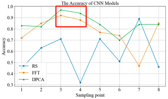
Figure 5.
Comparison of diagnostic accuracy between different feature extraction methods.
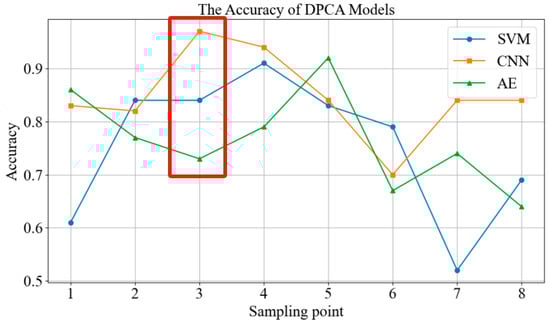
Figure 6.
Comparison of diagnostic accuracy of different deep learning networks.
Additionally, based on the comparison of Figure 5 and Figure 6, it is evident that the horizontal vibration signal at sampling point 3, which is the input end of the pump body, contributes the most to the diagnosis of diaphragm pump faults, with an average accuracy of 85.67%. Meanwhile, sampling point 6, the output end of the gearbox, contributes the least to the diagnosis of diaphragm pump faults, with an average accuracy of only 68.50%. Furthermore, sampling points 1, 2, 3, 4, and 5 show significantly better diagnostic performance when compared with sampling points 6, 7, and 8. This indicates that the vibration signals from the pump body and motor drive end are more effective in reflecting the fault status of the diaphragm pump compared with the vibration signals from the gearbox.
5. Conclusions
This study introduces the DMF fault diagnosis method as an innovative approach with which to address the limitations commonly associated with traditional diaphragm pump fault diagnosis techniques, characterized by incompleteness and inaccuracy. The DMF model demonstrates a significant improvement in diagnostic accuracy, achieving an impressive accuracy rate of 99.98%. Notably, the DMF model shows superior performance compared with individual models, with an average accuracy improvement of 9.09%. Specifically, it surpasses the sampling point 1-DPCA-AE model by 13.98% and the sampling point 4-DPCA-SVM model by 8.98%. A thorough analysis of multi-source information fusion methods reveals that the demodulation method is more effective in extracting vibration signal features from diaphragm pumps, while CNN excels at fault identification. Additionally, the study findings highlight the heightened sensitivity of vibration signals in the horizontal direction at the pump body’s input end for detecting diaphragm pump faults. Consequently, further experiments are warranted to enhance the robustness and generalizability of the research findings in the future. Future research will be carried in the direction of optimizing fault feature extraction methods, optimizing parameters of deep learning recognition models, and efficiently obtaining classification results in large amounts of data.
Author Contributions
Methodology, F.M., Z.S. and Y.S.; Software, F.M., Z.S. and Y.S.; Validation, F.M., Z.S. and Y.S.; Formal analysis, F.M., Z.S. and Y.S.; Investigation, F.M., Z.S. and Y.S.; Resources, Z.S.; Data curation, F.M. and Y.S.; Writing—original draft, F.M.; Writing—review & editing, Z.S. and Y.S.; Visualization, F.M. and Z.S.; Supervision, Z.S. and Y.S.; Project administration, Y.S.; Funding acquisition, Y.S. All authors have read and agreed to the published version of the manuscript.
Funding
This work was supported by the Natural Science Foundation of Shandong Province, China (no. ZR2021QE157) and the Open Foundation of State Key Laboratory of Compressor Technology (Compressor Technology Laboratory of Anhui Province) (no. SKL-YSJ202108).
Data Availability Statement
Data are contained within the article.
Conflicts of Interest
Author Fanguang Meng was employed by the company Zhejiang JingLiFang Digital Technology Group Co., Ltd. The remaining authors declare that the research was conducted in the absence of any commercial or financial relationships that could be construed as a potential conflict of interest.
References
- Zhao, K.; Lou, Y.; Peng, G.; Liu, C.; Chang, H. A Review of the Development and Research Status of Symmetrical Diaphragm Pumps. Symmetry 2023, 15, 2091. [Google Scholar] [CrossRef]
- Thalhofer, T.; Keck, M.; Kibler, S.; Hayden, O. Capacitive sensor and alternating drive mixing for microfluidic applications using micro diaphragm pumps. Sensors 2022, 22, 1273. [Google Scholar] [CrossRef]
- Zhou, C.; Jia, Y.; Bai, H.; Xing, L.; Yang, Y. Sliding dispersion entropy-based fault state detection for diaphragm pump parts. Coatings 2021, 11, 1536. [Google Scholar] [CrossRef]
- Feng, Z.; Xiong, X.; Wang, X. Fault diagnosis of diaphragm pump check valve based on impulse and cyclostationary analysis. In Proceedings of the 2021 33rd Chinese Control and Decision Conference (CCDC), IEEE 2021, Kunming, China, 22–24 May 2021; pp. 2092–2097. [Google Scholar]
- Li, X.; Chen, J.; Wang, Z.; Jia, X.; Peng, X. A non-destructive fault diagnosis method for a diaphragm compressor in the hydrogen refueling station. Int. J. Hydrogen Energy 2019, 44, 24301–24311. [Google Scholar] [CrossRef]
- Xu, X.; Guo, Z.; Liang, X. Intelligent fault diagnosis system design and implementation of diaphragm pump based on artificial intelligence. J. Phys. Conf. Ser. 2022, 2181, 012046. [Google Scholar] [CrossRef]
- Jia, Y.; Qingmao, L.; Xuyi, Y. The diaphragm pump spindle fault diagnosis using HHT based on EMD. Open Autom. Control Syst. J. 2015, 7, 640–645. [Google Scholar] [CrossRef]
- Chen, Y.; Huang, G.; Feng, Z. Early Fault Diagnosis of High Pressure Diaphragm Pump Check Valve Based on VMD-HMM. In Proceedings of the 2019 IEEE 8th Data Driven Control and Learning Systems Conference (DDCLS), IEEE, Dali, China, 24–27 May 2019; pp. 808–813. [Google Scholar]
- Wen, L.; Li, X.; Gao, L.; Zhang, Y. A new convolutional neural network-based data-driven fault diagnosis method. IEEE Trans. Ind. Electron. 2017, 65, 5990–5998. [Google Scholar] [CrossRef]
- Chen, H.; Jiang, B.; Ding, S.X.; Huang, B. Data-driven fault diagnosis for traction systems in high-speed trains: A survey, challenges, and perspectives. IEEE Trans. Intell. Transp. Syst. 2020, 23, 1700–1716. [Google Scholar] [CrossRef]
- Hongm, W.; Tian-You, C.; Jan-Liang, D.; Brown, M. Data driven fault diagnosis and fault tolerant control: Some advances and possible new directions. Acta Autom. Sin. 2009, 35, 739–747. [Google Scholar]
- MacGregor, J.; Cinar, A. Monitoring, fault diagnosis, fault-tolerant control and optimization: Data driven methods. Comput. Chem. Eng. 2012, 47, 111–120. [Google Scholar] [CrossRef]
- Li, W.; Zhu, Z.; Jiang, F.; Zhou, G.; Chen, G. Fault diagnosis of rotating machinery with a novel statistical feature extraction and evaluation method. Mech. Syst. Signal Process. 2015, 50, 414–426. [Google Scholar] [CrossRef]
- Rauber, T.W.; do Nascimento, E.M.; Wandekokem, E.D.; Varejão, F.M.; Herout, A. Pattern recognition based fault diagnosis in industrial processes: Review and application. Pattern Recognit. Recent Adv. 2010, 483–508. [Google Scholar] [CrossRef]
- Saufi, S.R.; Ahmad, Z.A.B.; Leong, M.S.; Lim, M.H. Challenges and opportunities of deep learning models for machinery fault detection and diagnosis: A review. IEEE Access 2019, 7, 122644–122662. [Google Scholar] [CrossRef]
- Carraro, G.; Pallis, P.; Leontaritis, A.D.; Karellas, S.; Vourliotis, P.; Rech, S.; Lazzaretto, A. Experimental performance evaluation of a multi-diaphragm pump of a micro-ORC system. Energy Procedia 2017, 129, 1018–1025. [Google Scholar] [CrossRef]
- D’Amico, F.; Pallis, P.; Leontaritis, A.D.; Karellas, S.; Kakalis, N.M.; Rech, S.; Lazzaretto, A. Semi-empirical model of a multi-diaphragm pump in an Organic Rankine Cycle (ORC) experimental unit. Energy 2018, 143, 1056–1071. [Google Scholar] [CrossRef]
- Gao, Z.; Cecati, C.; Ding, S.X. A survey of fault diagnosis and fault-tolerant techniques—Part I: Fault diagnosis with model-based and signal-based approaches. IEEE Trans. Ind. Electron. 2015, 62, 3757–3767. [Google Scholar] [CrossRef]
- Xu, W.; Jing, L.; Tan, J.; Dou, L. A multimodel decision fusion method based on DCNN-IDST for fault diagnosis of rolling bearing. Shock. Vib. 2020, 2020, 8856818. [Google Scholar] [CrossRef]
- Zeng, D.; Xu, J.; Xu, G. Data Fusion for Traffic Incident Detector Using DS Evidence Theory with Probabilistic SVMs. J. Comput. 2008, 3, 36–43. [Google Scholar] [CrossRef]
- Fu, Y.; Chen, X.; Liu, Y.; Son, C.; Yang, Y. Gearbox fault diagnosis based on multi-sensor and multi-channel decision-level fusion based on SDP. Appl. Sci. 2022, 12, 7535. [Google Scholar] [CrossRef]
- Wu, J.; Hu, K.; Cheng, Y.; Zhu, H.; Shao, X.; Wang, Y. Data-driven remaining useful life prediction via multiple sensor signals and deep long short-term memory neural network. ISA Trans. 2020, 97, 241–250. [Google Scholar] [CrossRef] [PubMed]
- Zhao, X.; Xu, L.; Li, J.; Fang, C.; Ouyang, M. Faults diagnosis for PEM fuel cell system based on multi-sensor signals and principle component analysis method. Int. J. Hydrog. Energy 2017, 42, 18524–18531. [Google Scholar] [CrossRef]
- Song, Y.; Ma, Q.; Zhang, T.; Li, F.; Yu, Y. Research on Fault Diagnosis Strategy of Air-Conditioning Systems Based on DPCA and Machine Learning. Processes 2023, 11, 1192. [Google Scholar] [CrossRef]


Disclaimer/Publisher’s Note: The statements, opinions and data contained in all publications are solely those of the individual author(s) and contributor(s) and not of MDPI and/or the editor(s). MDPI and/or the editor(s) disclaim responsibility for any injury to people or property resulting from any ideas, methods, instructions or products referred to in the content. |
© 2024 by the authors. Licensee MDPI, Basel, Switzerland. This article is an open access article distributed under the terms and conditions of the Creative Commons Attribution (CC BY) license (https://creativecommons.org/licenses/by/4.0/).