Abstract
In recent years, deep learning models have led to improved accuracy in industrial defect detection, often using variants of YOLO (You Only Look Once), due to its high performance at a low cost. However, the generalizability, fairness and bias of their outcomes have not been examined, which may lead to overconfident predictions. Additionally, the complexity added by co-occurring defects, single and multi-class defects, and the effect on training, is not taken into consideration. This study addresses these critical gaps by introducing new methodologies for analyzing dataset complexity and evaluating model fairness. It introduces the novel approach of co-occurrence impact analysis, examining how the co-occurrence of defects in sample images affects performance, and introducing new dimensions to dataset preparation and training. Its aim is to increase model robustness in the face of real-world scenarios where multiple defects often appear together. Our study also innovates in the evaluation of model fairness by adapting the disparate impact ratio (DIR) to consider the true positive rate (TPR) across different groups and modifying the predictive parity difference (PPD) metric to focus on biases present in industrial quality control. Experiments demonstrate by cross-validation that the model trained on combined datasets significantly outperforms others in accuracy without overfitting and results in increased fairness, as validated by our novel fairness metrics. Explainability also provides valuable insights on the effects of different training regimes, notably absent in prior works. This work not only advances the field of deep learning for defect detection but also provides a strategic framework for future advancements, emphasizing the need for balanced datasets and considerations of ethics, fairness, bias and generalizability in the deployment of artificial intelligence in industry.
1. Introduction
In the industrial manufacturing sector, the issue of surface defects on metal products presents a significant challenge. The repercussions of these defects are far-reaching, with financial implications and risks to company reputation being paramount. The first quarter of 2023 alone saw a dramatic increase in product recalls due to manufacturing defects in the US, with a 34% rise from the last quarter of 2022, amounting to 83.3 million units [1]. This alarming trend, highlighted in the “U.S. Product Safety And Recall Index” report by Sedgwick, underlines the critical nature of effective defect detection.
Traditionally, defect detection in manufacturing has relied heavily on human inspection, a method now increasingly recognized as error-prone. Studies, including those by Drury and Fox (1975), show human error contributes substantially to inspection inaccuracies, ranging between 20% and 30% [2]. The evolution of deep learning models for defect detection has marked a transformative shift in this domain, with recent deep learning models [3,4,5,6,7,8] increasingly used for industrial inspection to automate the identification of specific defect classes, provide valuable insights into production process issues, and allow for timely interventions that can prevent costly machine or process shutdowns.
Despite these advances in automating defect detection, there persists a notable gap in the investigation of the generalizability of such solutions, their fairness and the presence of bias, which may adversely affect the reliability of results. Moreover, the literature has not examined the role of the number, uniqueness and co-occurrence of defects in datasets and their effect on training, augmentation and final outcomes. Images of metal surfaces may either contain a single or multiple classes of defects, in some cases co-occurring: e.g., an image may contain multiple defects (referred to hereafter as “multi-class”), amongst which some may also appear uniquely in other images (referred to hereafter as “single-class”). This may confound training and complicates our understanding of the distinct impacts of data augmentation techniques on single-class versus multi-class image datasets. Common augmentation strategies, including rotation, scaling, flipping, cropping, and adjustments in brightness or contrast, are typically applied uniformly across datasets. However, the uniform application of augmentation techniques may not be optimally effective for datasets with diverse characteristics, especially including both single and multi-class images with co-occurring defects. If certain defects co-occur in single and multi-class images, their number of instances is likely to increase in an unbalanced manner after the application of uniform data augmentation. This is likely to lead to overconfident predictions, biased and unfair performance and lack of generalizability, even when otherwise high-performing optimized models are deployed. For example, 30% of the widely used GC10-DET dataset [3,4,5,8], also examined in this work, comprises multi-class images with varying co-occurrence defects. This disparity raises a crucial question about the adequacy of current augmentation methods used in recent papers and the potential need for more tailored approaches to enhance dataset stratification and thereby improve model performance.
This study, therefore, embarks on a comprehensive, systematic investigation of the nuanced impact of diverse training regimes on unbalanced, real-world datasets, with a focus on generalizability, fairness and bias. It introduces a novel framework of co-occurrence impact analysis, examining in depth how the presence of single or multiple classes of defects in the same image and the co-occurrence of defects influence detection performance. It applies tailored augmentation and balancing strategies, leading to truly balanced and fair training datasets, which are shown to lead to improved, generalizable performance. Explainability methods are used to demonstrate that our proposed approach of fair and balanced training allows models to focus on the actual defect areas more effectively than commonly used augmentation solutions, resulting in robust and accurate outcomes. The use of explainability not only enhances the transparency of the defect detection models but also aids in identifying potential areas for further bias mitigation and model improvement. This work also redefines fairness and bias metrics, namely the disparate impact ratio (DIR) and positive parity difference (PPD), by concentrating on true positive rates (TPR). It thus shifts the focus of fairness and bias metrics to the accurate detection of defects in real-world datasets, with under-represented and co-occurring defects in single and multi-class images. Thus, our work contributes to the field by providing an in-depth examination of the effect of dataset bias through co-occurring or under-represented defects, the effect of diverse data balancing approaches and the re-definition of fairness and bias metrics for industrial applications.
In order to objectively assess the effect of training strategies, fairness, bias and generalizability, it examines a fixed model to ensure consistency across the experimental conditions. As the focus of this work is not the development of a new defect detection model, it uses a variant of the commonly deployed YOLOv5 model. A large number of recent works use YOLOv5 as their basis [3,5,6,7,8,9,10], and more recently YOLOv7 [4]. Although YOLOv7 outperforms YOLOv5 in terms of performance, this is only possible on high-performance GPUs, which may not be easily accessible to industry. For this reason, and the fact that the majority of recent works use YOLOv5 due to its appropriateness for real-world conditions, we fix our model to the more computationally efficient YOLOv5s. The resulting conclusions regarding training balancing strategies and dataset management are expected to apply to all models used for defect detection, as they concern dataset management, preprocessing and experimental setup. The overarching objectives and contributions of this research are multi-fold:
- Analyze the impact of training data diversity by comparing the performance of models trained on single-class images with those trained on multi-class images, to investigate how data representation influences model performance.
- Systematically explore the effectiveness of transfer learning and fine tuning in enhancing model performance for specific scenarios with mismatched datasets, i.e., when a pre-trained model is trained on data that is different from the testing data.
- Investigate model bias and fairness by a critical and quantitative assessment of fairness and bias in models trained on different data types to detect various defects.
- Bridge theory with practical application in industrial quality control by offering a practical framework and insights into how DL can be practically applied in industry, providing best practices for industrial quality assurance.
This paper is structured as follows: Section 2 presents recent works on metal surface defect detection. Section 3 presents the dataset that is examined in depth in this work. The methods used for the detection of defects are presented in Section 4: the systematic exploration and preparation of the datasets to be used in our experiments is detailed in Section 4.2, while Section 4.3 describes the model used. Section 4.4 presents the methods used for the measurement of fairness, bias and explainability in the proposed experiments. The experimental setups and results are presented in Section 5, while Section 6 focuses on their outcomes in terms of generalizability, fairness, bias and the role of explainability. An in-depth discussion of all experimental outcomes takes place in Section 7, while conclusions are drawn in Section 8, along with plans for future work.
2. Related Work
The recent advancements in machine learning for metal surface defect detection are marked by diverse approaches and significant results. Xiaoming Lv et al. [3] combined the SSD framework with hard negative mining, introducing a robust method for defect detection on metallic surfaces, showing notable accuracy improvements. Yang Wang et al. [4] enhanced YOLOv7 for steel strip surface defects, focusing on small targets with enhanced feature pyramid and attention mechanisms, achieving remarkable precision. Ping Liu et al. [11] optimized Faster R-CNN for mechanical design products, improving feature extraction and pooling algorithms, demonstrating increased defect detection efficiency. Kun Wang et al. [5] improved YOLOv5 using data augmentation and an asymmetric loss function, specifically targeting small-scale defects, and observed substantial accuracy gains. F. Akhyar et al.’s [6] forceful steel defect detector combined Cascade R-CNN with advanced techniques, exhibiting superior defect detection capabilities in complex environments. Ling Wang et al. [9] enhanced YOLOv5 with a multi-scale block and spatial attention mechanism that excelled in real-time defect detection. Yu Zhang et al.’s [7] integration of the CBAM mechanism into YOLOv5s specifically addressed bottom surface defects in lithium batteries, offering significant detection improvements. Manas Mehta’s model based on YOLOv5 [10], incorporating ECA-Net and BiFPN, showcased enhanced real-time steel surface defect detection. Lastly, Chuande Zhou et al. [8] improved YOLOv5s with CSPLayer and GAMAttention and effectively detected small metal surface defects, marking a leap in detection sensitivity.
The reviewed papers collectively emphasize the critical role of surface defect detection in materials like steel, metal [3,4,5,6,8,9,10,11] and lithium batteries [7] for industrial quality control, primarily through the use of advanced deep learning models, particularly convolutional neural networks (CNNs). This shift towards AI-based approaches is evident in their experimentation with YOLO (You Only Look Once) and R-CNN (region-based convolutional neural networks) model variants [4,5,6,8,9,10,11], affirming their effectiveness in object detection. Notably, each study introduces enhancements to models such as YOLOv5, Faster R-CNN, or YOLOv7, focusing on increasing accuracy and detection speed, especially for small defects [4,5,8]. The incorporation of attention mechanisms and feature fusion techniques [4,6,7,8,10] is a common strategy to improve performance on challenging defect types. Moreover, these papers frequently utilize standard benchmarking datasets like NEU-DET and GC10-DET [3,4,5,6,8,9,10] for training and benchmarking, employing metrics such as mean average precision (mAP), precision, recall, and accuracy for evaluation.
In the context of real-time production, modified versions of the YOLO model, including YOLOv5 and its derivatives, are lauded for their efficiency and high accuracy [4,5,7,8,10]. Optimized Faster R-CNN models also show promise [6,11], achieving a commendable balance between detection speed and accuracy. Papers introducing custom architectures or specific model enhancements, like AFF-YOLO [10] and FDD [6], demonstrate practical effectiveness in real-time scenarios. Addressing the challenge of small surface defects, several methods stand out. The integration of attention mechanisms, such as the convolutional block attention module (CBAM), and feature fusion techniques [7] significantly enhance the model’s capability to focus on small defects. Data augmentation and scaling techniques aid in better representing and detecting minute defects [5]. Furthermore, optimizing model architecture by adding specific layers or adjusting the network caters [5] more effectively to small target detection. Lastly, tweaking the loss function to prioritize small-sized defects [4] has also been shown to bolster detection accuracy.
The state-of-the-art (SoA) methods described above have significantly improved the accurate detection of small defects on metal surfaces; however, the generalizability, fairness and bias of these solutions have not been examined, nor the effect of diverse training regimes on performance. This study aims to bridge that gap, by investigating the intricacies of training machine learning models, focusing on the effects of class composition diversity on model efficacy, bias, and fairness, while employing explainability to determine the reliability of results. Such an investigation can a reveal lack of generalizability and fairness, as well as biased performance for co-occurring or under-represented classes of defects. A framework of systematic data balancing, taking into account the co-occurrence of defects in single and multi-class images and the under-representation of others, has the potential to provide truly balanced and varied training datasets. In addition to the goal of dataset balance, data augmentations should reflect real-world conditions that occur in industrial settings. Our work shows that the introduction of our new framework for dataset preparation and model training, as well as the measurement of tailored fairness and bias metrics, can address these issues effectively. This approach can thus set the basis for improving the performance of any model, rendering it more fair, generalizable and unbiased, aspects of great importance in applications such as industrial defect detection.
In order to provide results relevant to the recent SoA, the GC10-DET benchmarking dataset [3] is examined (Section 3), as it is used in many of the related works. Moreover, in order to obtain objective comparisons of fairness, bias and generalizability, these aspects are investigated for one fixed model, namely YOLOv5s. This choice is made as models in the YOLO family, and particularly YOLOv5, are most often encountered in the literature, due to its appropriateness for industrial applications [3,5,6,7,8,9,10]. In this work, we use a small version of YOLOv5, i.e., YOLOv5s, which has the same architecture but is more computationally efficient. It should be emphasized that this work does not aim to provide direct comparisons with one of the many YOLO variants from the literature mentioned above, as its aim is to provide more general insights on fairness, bias and generalizability on the family of YOLO models, rather than on one of its specific variants. The results of this work regarding a novel training framework, new metrics for fairness and bias, and a new paradigm for explainable, fair, defect detection, apply equally to any detection model, as they concern dataset management and pre-processing. Thus, going beyond the SoA, this work will examine:
- Generalization under different training regimes: How does generalization change when training on data with single-class images compared to multi-class images?
- Bias in training data analysis: Does training a DL model on a single class of defects introduce significant bias towards that class in terms of prediction accuracy when testing on images including multiple defects? How does the inclusion of multiple defect classes in the training data influence bias towards images containing defects of a single class?
- Fairness assessment: How fair is a machine learning model in classifying different types of defects when trained on single- versus multi-class data, and tested on data containing multiple classes? Can fairness in defect classification be improved by diversifying the types of defects in the training dataset, and if so, to what extent?
- Comparative analysis: What are the key differences in terms of accuracy, precision, recall, F1 Score when a model is trained on single- versus multi-class data? How does the model’s ability to detect infrequent defects differ between the training approaches?
- Methodological exploration: What are the most effective strategies and metrics for evaluating model generalization, bias and fairness in the context of defect detection? How do different training strategies influence the generalization, bias and fairness?
- Practical implications: What are the practical implications of the findings for industrial defect detection? How can the insights from this research inform the design and training of more robust and fair DL models for defect detection in various applications?
3. Dataset Description
The GC10-DET dataset (Figure 1), introduced in [3], is a vital resource of metal sheet defect images. Originating from a real industrial setting, it includes a diverse spectrum of ten distinct surface defect types on steel sheets. These include punching (Pu), weld line (Wl), crescent gap (Cg), water spot (Ws), oil spot (Os), silk spot (Ss), inclusion (In), rolled pit (Rp), crease (Cr), and waist folding (Wf). The published dataset originally comprised 3482 images, including 1398 images augmented by horizontal flipping. Our study uses only the 2084 original TrueColor images ( pixels), since it aims to study the effect of image augmentations in a controlled manner, depending on the number of classes present in the images. For methodological transparency and technical accuracy [3], it is pertinent to detail the equipment used in the dataset’s compilation. The image capturing device is a Teledyne DALSA LA-CM-04K08A camera, renowned for its precision in industrial applications. The lens employed is a Moritex ML-3528-43F. The images are corrected under a direct current (DC) light source. The images in this dataset may contain one or more instances of commonly encountered defects, described below. The presence of one or multiple classes of labels in the training data is examined in depth in Section 4.2 and Section 5, as it affects training dataset balance and subsequently the performance of the examined model.
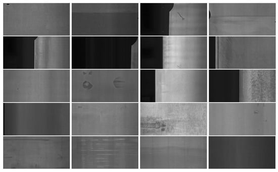
Figure 1.
Sample images from the GC10-DET dataset with 2 examples of each defect: punching hole, welding line, crescent gap, water spot, oil spot, silk spot, inclusion, rolled pit, crease, waist folding.
4. Methods
4.1. Overview of the Proposed Framework
The main proposition and contribution of this work is a strategic bias mitigation framework to support the fair, generalizable, unbiased implementation of DL models in real-world applications. An overview of the framework is shown in Figure 2, and its different stages are detailed in Section 4.2, Section 4.3 and Section 4.4. In order to achieve fair, generalizable, unbiased detection of defects and other anomalies, it is recommended to split the data into groups with the same and different multiple defect types. In the case of single-class defects, the dataset can be balanced through typical data augmentation methods. In the case of multi-class defects, attention should be paid to particular instances of defects that need to be individually balanced. In the case of real-world conditions, such as those encountered in industrial settings, we also recommend applying augmentations that mimic noise present in the real world. The remaining steps of our pipeline follow the traditional steps of any machine or deep learning implementation, with training, validation, testing split, modeling and prediction steps. We also adapt fairness and bias metrics, and propose an in-depth examination of results for fairness and bias through the related metrics and explainability in order to adapt dataset management when needed.
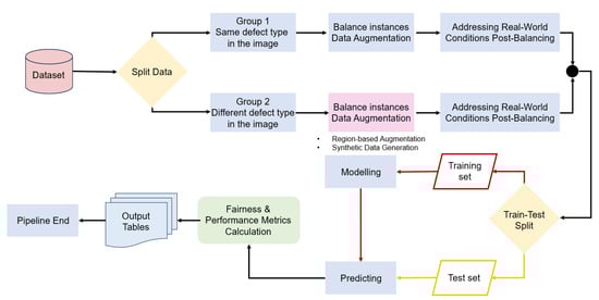
Figure 2.
The flowchart of our framework for bias mitigation in single-class and multi-class detection models.
4.2. Dataset Preparation, Analysis
In this section we describe the steps taken in order to create balanced datasets when faced with co-occurring or infrequently occurring defects in single and multi-class image data.
4.2.1. Balanced Datasets Creation
The flowchart of Figure 3 describes the systematic procedure we follow in preparing our data for experimental analysis, detailed in this section.
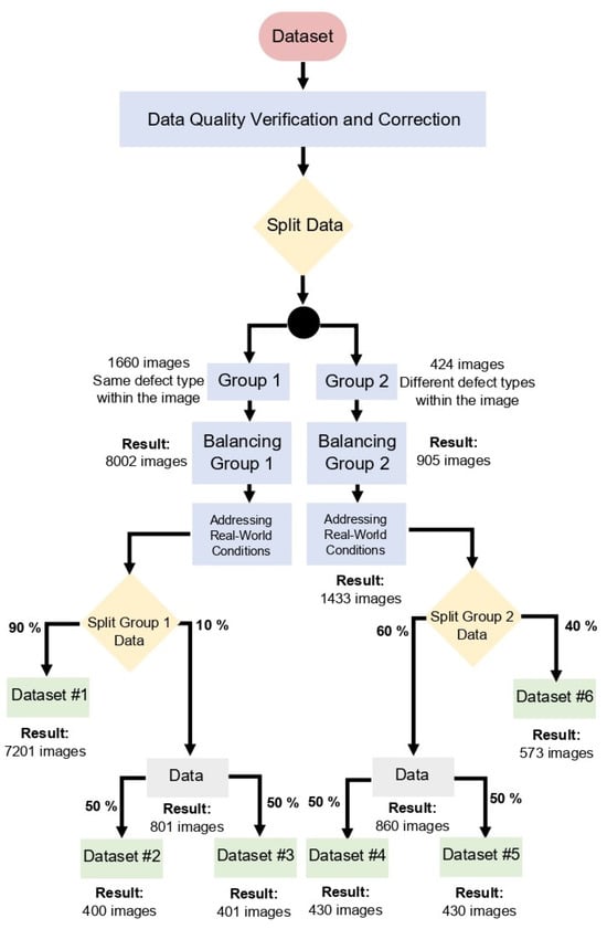
Figure 3.
Flowchart for preparing image datasets for experimental use. Attention is paid to co-occurring defects in single and multi-class images, as well as under-represented data. Data augmentations also take place to mimic real-world industrial conditions.
The dataset contains a mix of single and multi-class images, with defects that may co-occur in single and multi-class images, may appear uniquely in either case, or may be rare. Some sample images of single and multi-class images are shown in Figure 4.
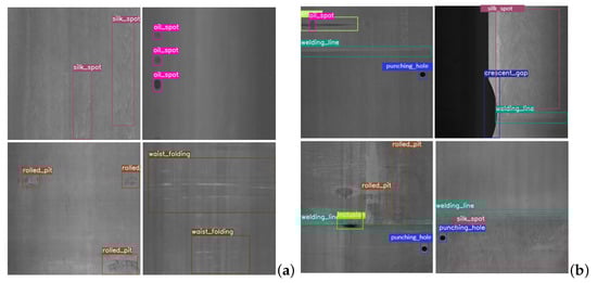
Figure 4.
Examples of images with (a) a single class and (b) multiple classes of metal defects.
In addition to including rare and co-occurring defect classes, this dataset faces three prevalent issues: misclassified or incorrect labels, missing labels, and inconsistent labeling, so it is good practice to conduct a manual review and correction of the labels for each image to ensure accuracy and consistency. After this meticulous process, the dataset is refined to a total of 3243 instances, whose color labels are shown in Figure 5 and the resulting class (defect) distribution in the “cleaned” dataset before data balancing is shown in Figure 6a. Next, the dataset is split into two groups. Group 1 comprises 2265 instances with the same type of defect (as in Figure 4a), with the distribution across the various defect classes illustrated in Figure 6b. In contrast, Group 2 consists of 978 instances, each containing multiple, different defect types (as in Figure 4b), whose distribution is detailed in Figure 6c. Group 1 started with 1660 images, while Group 2 with 424 images, but a methodical balancing process augmented Group 1 from its original count to 8002 images, and Group 2 to 905 images. The distribution of instances in Group 1 and Group 2 after balancing is illustrated in Figure 7a and Figure 7b, respectively. This significant augmentation is achieved using horizontal flips, vertical flips, rotations at angles of 30, −30, 45, −45, 60, −60, and 90 degrees, random crops, and adjustments to image brightness to simulate darker conditions.
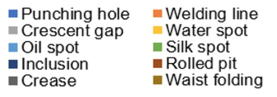
Figure 5.
Colors used to represent each class of the GC10-DET dataset.
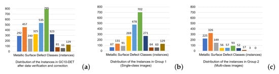
Figure 6.
(a) Distribution of the instances in the entire GC10-DET dataset after data verification and correction, before balancing. (b) Distribution of the instances in Group 1 (Single-class images) after data verification and correction, before balancing. (c) Distribution of the instances in Group 2 (multi-class images) after data verification and correction, before balancing. There is high class-imbalance in both single and multi-class images.
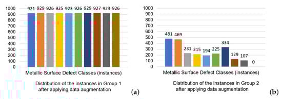
Figure 7.
Instance distribution in GC10-DET after data augmentations for balancing classes. (a) Single-class images can be uniformly balanced. (b) Data balancing for multi-class images requires additional attention to co-occurring and infrequently occurring defects.
Finally, both groups are modified by variations that mimic real-world conditions: additive and multiplicative Gaussian noise, local brightness fluctuations, local contrast adjustments, dodging and burning, and linear mapping to modulate brightness, are applied to 15% of the instances within each class. These data augmentations are chosen among those commonly used in the literature, as they best replicate real-world conditions. They are described in detail in Appendix A. Figure 8a shows that these augmentations can achieve perfect balance for single class images, while Figure 8b shows these augmentations improve dataset balance for Group 2, multi-class images, without achieving perfect balance due to the high variability of class instances: some defect classes are rare, while others occur or co-occur in different amounts in the data.
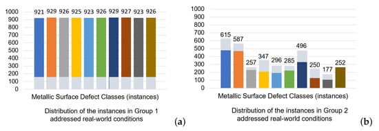
Figure 8.
Instance distribution in GC10-DET after augmentations addressing real-world conditions for (a) Group 1: single class images. The augmentations directly lead to a balanced dataset. (b) Group 2: multi-class images. The augmentations improve dataset balance but do not lead to a perfectly balanced dataset due to the high variability in the occurrences and co-occurrences of class instances.
Subsequently, Group 1 is partitioned, with 90% forming Dataset #1, while the remaining 10% is distributed evenly to create Datasets #2 and #3. For Group 2, a similar stratification is suggested, with augmentations taking place, but also keeping the original unmodified images in the dataset, in order to increase the number of instances. The defect ‘waist folding’ is unique in that it does not co-occur with other defect types, so it is absent from Group 2, which comprises images with multiple defects. To address this, images from Group 1 with ‘waist folding’ undergo augmentation, resulting in 252 instances of this defect, which are then added to Group 2 for a more comprehensive representation of defect types across both groups (Figure 8b). So, the number of images in Group 2 after addressing real-world conditions is 1433. Subsequently, this group is partitioned, with 40% forming Dataset #6, while the remaining 60% is distributed evenly to create Datasets #4 and #5. This careful, detailed, pre-processing regimen is designed to prepare the data for rigorous experimental testing and investigation of fairness, bias and generalization.
4.2.2. Data Exploration
In the realm of industrial manufacturing, understanding the intricate relationships between different types of defects is crucial for enhancing quality control measures. This study utilizes heatmap visualization (Figure 9) to dissect and comprehend the co-occurrence patterns of various defects in a multi-class image dataset (Group 2), providing a compelling visual summary of defect interdependencies.
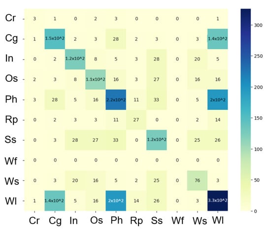
Figure 9.
A co-occurrence matrix of different classes labeled in Group 2 (before balancing stage).
A pronounced co-occurrence is thus revealed between crescent gap (Cg) and welding line (Wl), as well as punching hole (Ph) and welding line (Wl), indicating these defects frequently appear together within the same samples. This strong relationship suggests a possible shared causal factor or a sequence in the manufacturing process that predisposes the occurrence of one defect when the other is present. Other moderate co-occurrence relationships are observed among different pairs of defects such as crescent gap (Cg) and punching hole (Ph), inclusion (In) with both silk spot (Ss) and water spot (Ws), and oil spot (Os) with silk spot (Ss), water spot (Ws), and welding line (Wl). These moderate co-occurrences suggest that, while these defects are less frequently associated, there is still a significant relational trend that warrants further investigation. The heatmap’s diagonal, which reflects the frequency of each individual defect type, revealed high values. This pattern is not only expected, but also vital for understanding the overall occurrence rate of each defect within the dataset. An intriguing aspect of the findings is the isolated occurrence of waist folding (Wf), which did not co-occur with any other defect type. This unique pattern highlights the distinct nature of waist folding (Wf) compared to other defects and may prompt a specialized inspection process. This study also points to potential skewness in the data. The disproportionate prevalence of certain defects, particularly welding line (Wl), suggests that some are overrepresented. This imbalance can have profound implications for training, as it may bias models towards overrepresented defects. Hence, there is a need for strategic approaches such as data augmentation or a rebalanced sampling technique to ensure a fair representation of all defect types.
4.3. Defect Detection by YOLOv5s
In the field of object detection, there are two prominent approaches: two-stage [12] and single-stage deep learning models [13]. Single-stage models, exemplified by YOLO (You Only Look Once) [7,13], achieve accurate and speedy online object detection the process by combining object localization and detection into one unified model. In this work, we will focus in depth on various aspects of the performance of metal defect detection on GC10-DET using the YOLOv5 model, as it is frequently used in the field [3,5,6,7,8,9,10], due to its very good balance of computational cost and performance, making it a leading choice in scenarios where both factors are crucial. In this work, we examine YOLOv5s, which has the same architecture as YOLOv5, but is smaller, in order to be more computationally efficient, making it a realistic choice for industrial and other real-world applications.
YOLOv5 firstly comprises the Backbone, functioning as the core framework, which employs the innovative New CSP-Darknet53 structure. This design is a refined adaptation of the Darknet architecture, which was foundational in earlier iterations, signifying a progressive evolution in its structural design. Secondly, the Neck serves as a critical intermediary, seamlessly connecting the Backbone to the Head. In this capacity, YOLOv5 integrates the SPPF and New CSP-PAN structures, ensuring a fluid and effective transition of data within the model. Lastly, the Head is pivotal for producing the final output, employing the YOLOv3 Head mechanism. This strategic composition of the model’s structure demonstrates a balanced fusion of proven and novel elements, culminating in a robust and highly capable online object detection system.
In this work, YOLOv5 is used in various training regimes, both trained from scratch and using transfer learning and fine-tuning. The core concept of transfer learning centers around using a pre-trained model and adapting it to a different task. This adaptation is achieved by selectively training only the uppermost layers of the model. In this structure, the lower layers are dedicated to extracting features, while the upper layers focus on classifying and detecting these features. The effectiveness of this approach is greater when the pre-trained model has been trained on a general enough dataset or when the original and new tasks are closely related, aspects which are investigated in Section 5.
Performance Metrics: To evaluate experiments, we employ widely used performance metrics, which are also a critical part of assessing bias and fairness in the context of generalization. Here TP represents true positives, TN true negatives, FN false negatives and FP false positives.
Recall measures the proportion of actual positives correctly identified by the model:
Precision assesses the proportion of positive identifications that were actually correct:
F1 Score combines precision and recall, providing a single measure of model accuracy that offers a comprehensive view of the model’s performance in terms of both identifying relevant instances and minimizing false alarms, with F1 from 0 (worst) to 1 (best):
Mean average Precision (mAP) is calculated as the mean of the Average Precisions (AP) for different object classes, considering Intersection over Union (IoU) threshold (overlap between the predicted and actual target areas) from to .
4.4. Generalization, Bias, Fairness, Explainability
Several approaches are used to gauge the generalizability of YOLOv5s for metal defect detection by methodically evaluating their performance on previously unseen data.
Generalization: k-fold cross-validation, specifically a 5-fold cross-validation, is used to assess the robustness and unbiased performance of the model across various data subsets. This involves dividing the dataset into five equal parts, where each part is used as a validation set while the remaining data serve as the training set. The model’s stability and generalizability are thus rigorously evaluated using the outcomes from all five folds.
Bias: The presence of bias in training datasets can result in models that demonstrate high performance on training data but significantly underperform when encountering different data. This discrepancy arises because the model has learned patterns and associations that are overly specific to the training set, or over-represented groups in it, lacking the necessary generalizability to handle diverse or novel data instances effectively. Several approaches are employed to effectively identify bias and mitigate its effects.
Data distribution analysis: Evaluating the training data class distribution is essential to identify potential biases, since unequal class distribution can lead to bias. As detailed in Section 4.2, careful dataset splitting and augmentations can lead to more balanced datasets.
Confusion matrices reveal performance across different defects. A model biased towards certain classes (e.g. over-represented or co-occurring defects) will show significantly higher performance on them compared to others.
Class-wise performance metrics: Bias is also detected from recall, and F1 scores calculated separately for each class. Class-wise performance metrics can identify potential biases towards certain defects, leading to more objective and accurate performance assessment.
Fairness: The Disparate Impact Ratio (DIR) is a widely acknowledged measure for evaluating the fairness of predictions across different demographic groups [14]. It assesses the proportionality of true positives (TP) without considering the accuracy of these predictions [15]. However, certain contexts necessitate a fairness assessment based on the model’s sensitivity, also known as true positive rate (TPR) particularly where false negatives carry significant consequences, such as in healthcare diagnostics or, in the case of this work, quality control in manufacturing [16]. The TPR is essentially the same as recall, defined as:
In our framework, we define a specialized DIR that focuses on TPR, to measure equality of opportunity in the correct identification of positive instances in privileged and unprivileged groups. Here, privileged groups refer to defects well represented in the training data, and unprivileged groups represent defects with few samples. The specialized DIR is:
A DIR TPR value deviating from unity indicates a disparity in model sensitivity, which may reflect a bias in detecting true positive instances between the compared classes. The interpretation of the specialized DIR based on TPR, DIR TPR essentially reflects how well the model identifies true positives in both privileged and unprivileged groups as follows:
Value of 1: A DIR TPR value of 1 suggests an ideal scenario where the model demonstrates equal sensitivity towards both groups. It indicates that members of both groups have an equal likelihood of being correctly identified when they are indeed positive cases. This scenario reflects the achievement of equality of opportunity in terms of model performance.
Value greater than 1: A value greater than 1 implies that the model is more sensitive towards the unprivileged group. This may suggest over-prediction or higher recall for the unprivileged group compared to the privileged group.
Value less than 1: Conversely, a value less than 1 indicates that the model is less sensitive towards the unprivileged group. This scenario reveals a potential bias against the unprivileged group, suggesting that the model may not be detecting positive instances in this group as effectively as it does in the privileged group.
Practitioners should aim for a DIR TPR value close to 1, signifying equal treatment of all groups by the model in terms of correctly identifying positive instances. Values deviating significantly from 1 warrant a deeper investigation into the model’s training data, feature selection and potential inherent biases.
True positive rate differences (TPR Diff), i.e., the difference in TPR between privileged and unprivileged groups, highlights disparities in TPR, i.e., model sensitivity. It is directly linked to the principle of “equality of opportunity” in predictive outcomes [16,17]:
Moreover, the interpretation of TPR Diff must be contextually grounded: in domains like quality control, the cost of false negatives is high, so equitable TPRs are essential [18].
Predictive Parity Difference (PPD) is a fairness metric in the realm of multi-class predictive modeling that assesses the balance in prediction precision between different demographic groups. In a multi-class setting, this involves averaging the precision across classes within each group before determining the disparity. PPD can thus measure the disparity in precision between privileged and unprivileged groups across multiple classes.
Definition and calculation of PPD in multi-class context: Precision(P) for each class in a multi-class setting is determined separately. In a group, the Average Precision (AP) for a group, i.e., the mean of precisions calculated for each class within that group, encompasses the likelihood of correct positive predictions across various classes. PPD is then computed as the difference between average precision of the privileged and unprivileged groups:
In multi-class models, PPD ensures that no group is consistently receiving less accurate positive predictions across a range of classes. Significant PPD values indicate a skew in precision, suggesting that one group’s positive outcomes might be systematically over- or under-predicted compared to another. Particularly in fields where classification spans multiple categories (such as defect types in manufacturing), understanding PPD is vital to ensuring that all classes are treated fairly across different demographic groups [15,16,17].
Explainability via Eigen Class Activation Mapping (Eigen-CAM): Eigen Class Activation Mapping [19] is a model explainability tool tailored for convolutional neural networks (CNNs), aiming to elucidate how models interpret visual data to make predictions. Eigen-CAM serves as a qualitative indicator of the training process, helping determine the adequacy of training setups, the need for additional data augmentation, and identifying potential focus errors in the model’s predictions. Eigen-CAM stands out for its simplicity and easy integration, without the need for re-training or layer modifications. It computes and visualizes the principal components of features from convolutional layers, creating heatmaps overlaid on the input image, to highlight areas with the most significant layer activations. These visualizations can vary, showing heatmaps from different layers or a combined heatmap to underline the image’s overall focal points. Unlike class-specific techniques such as gradient-weighted class activation mapping (Grad-CAM), Eigen-CAM is a class-agnostic method that facilitates the visualization of features that CNNs leverage to make decisions, regardless of the classification output [20]. This is especially pertinent in our work, where multiple classes exist within single images, as it bypasses the need to segment explanations by class. Furthermore, Eigen-CAM is beneficial in circumventing the ambiguity that arises in multi-label scenarios where several defect classes may spatially overlap or closely interact within an image. Class-specific techniques can yield convoluted insights that are challenging to disentangle, whereas Eigen-CAM sidesteps this issue, providing a singular, coherent heatmap.
5. Experiments
Four different experimental setups take place to compare different training and data balancing regimes, transfer learning, and assess fairness, bias and generalizability. The results of each experiment in terms of performance metrics (precision, recall, mAP, F1 Score) are analyzed and discussed in each subsection that follows, including comparisons among approaches. The discussion of the Experiment 3 results also examines fairness, bias and generalizability, as these are the goals of that experiment, while an in depth discussion of generalizability, fairness and bias, using confusion matrices and fairness and bias metrics, respectively, follows in Section 6. The results are further discussed in detail in Section 7.
Data augmentation and hyperparameters throughout all experiments adhere to the default data augmentation techniques and hyperparameters for the training of YOLOv5s recommended by Jocher et al. in [13], with specific modifications to accommodate our experimental design. The details of our experimental setup are listed in Table 1.

Table 1.
Experimental setup: YOLOv5s fixed hyperparameters.
The HSV adjustments we made were: hue: , saturation: , value: . Our image augmentations parameters were: rotation degrees: 0, translate: 0.1, scale: 0.5, shear: 0, perspective: 0, flip up-down: 0, flip left-right: 0.5, mosaic: 1.0, mixup: 0.0, copy-paste: 0.0. Our modifications included setting the batch size to 32 and the image resolution to , while the maximum number of epochs for fine-tuning was capped at 150. Such adjustments were made to align the training process with our computational resources and the specific requirements of our datasets.
5.1. Experiment 1: Baseline Model—Fine-Tuning Pre-Trained YOLO on Single-Class Images
The objective of Experiment 1 was to establish a foundational performance benchmark for an object detection model trained exclusively on images containing single object classes (Figure 10 Left). It aimed to assess the model’s ability to generalize from a training set composed solely of single-class images to a testing set that includes both single and multi-class images. The computational demands of training YOLOv5s were met by employing an NVIDIA A100-SXM4-40GB with 40514MiB provided by Google Colab.
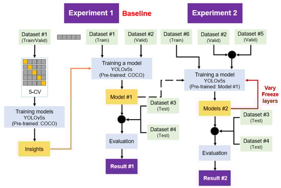
Figure 10.
Flowchart of model training and evaluation experiments. Left: Experiment 1 baseline model, with a pre-trained model and fine-tuning using single-class images. Right: Experiment 2, exploring fine-tuning the baseline model using multi-class images.
Dataset #1 (7201 single-class images) was used to fine-tune YOLOv5s pre-trained on the COCO dataset for more robust feature extraction from the outset. To ensure the model was not overfitting and to gauge its predictive robustness, five-fold cross-validation was applied to the training data. Insights obtained from this process were critical in fine-tuning the model’s parameters and preparing it for the final training phase. Subsequently, the entire Dataset #1 was employed to fully train the model, exploiting the full spectrum of data available post-cross-validation. This strategic approach aimed to maximize the model’s performance by leveraging the insights gained during the cross-validation phase. For the validation of the model’s hyperparameters, Dataset #2, containing 400 single-class images, was used. The performance and generalizability of the model were then tested using a combination of Dataset #3, with 401 single-class images, and Dataset #4, comprising 430 multi-class images. This mix allowed for a comprehensive evaluation of the model’s capability to detect objects across varied scenarios, which is paramount for practical applications.
Experiment 1 Results (Baseline, 5-Fold Cross-Validation): The five-fold cross-validation results from YOLOv5s for Experiment 1 in terms of precision, recall, F1 score, and mean average precision (mAP) at different intersection over union (IoU) thresholds are summarized in Table 2, where it can be seen that its performance remains consistent, indicating that there is no overfitting. Average recall rates are slightly lower than precision, pointing to a potential area for improvement in the model’s ability to detect all relevant instances. Average mAP50-95 scores across a range of IoU thresholds also remain consistent; however, they are lower than average mAP50, suggesting that the model struggles to maintain high precision when stricter criteria for defect detection are applied.
Table 2.
Average performance metrics values in 5-fold cross validation: precision, recall, F1 score, mAP50, mAP50-95 all show there is no overfitting.
A comprehensive view of the model’s performance in defect detection across the different classes of defects is provided in Table A1, Table A2, Table A3, Table A4 and Table A5 in Appendix B. One of the standout observations is the model’s robust ability to detect specific types of defects, notably crescent gap (Cg) and waist folding (Wf), which consistently show high precision, recall, and F1 scores across all folds. Such performance suggests that the model has effectively learned to identify the distinguishing features of these defects, possibly due to their distinct characteristics or adequate representation in the training set. Other defects like crease (Cr) and welding line (Wl) also exhibit commendable detection rates, although they display some variability across different folds. However, the model faces challenges with certain defects, particularly inclusion (In) and silk spot (Ss), which consistently score lower across all evaluation metrics. This could be attributed to their complexity, their resemblance to non-defective areas, similarities with the background, variability within the class, difficulty in distinguishing this class from others, or extremely small scale illustrated in Figure 11. The variable performance with defects like oil spot (Os),punching hole (Ph), and rolled pit (Rp) further suggests that, while the model is capable of detecting these defects to a certain extent, there is notable room for improvement.
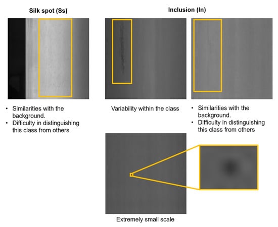
Figure 11.
The yellow box in each image shows different cases of challenging defects (from left to right): Silk spot defect very similar to the background and other classes; Inclusion defects with high intra-class variability, the one on the right also similar to the background and other defect classes; Silk spot defect of an extremely small scale.
Training, validation and testing performance losses and accuracy curves, as well as precision, recall, mAP5 and mAP50-95, are estimated for different folds to examine overfitting. They are represented with different colors for each fold, explained in Figure 12, for the plots in Figure 13, Figure 14, Figure 15, Figure 16 and Figure 17.
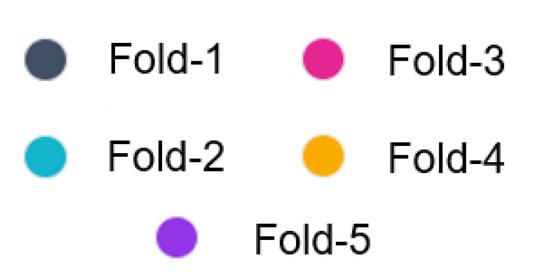
Figure 12.
Different colors to represent the different folds in the 5-fold cross validation experiments on generalizability.
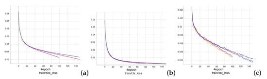
Figure 13.
Training (a) box, (b) class, (c) object losses in 5-fold cross validation, with each different color corresponding to a fold as in Figure 12.
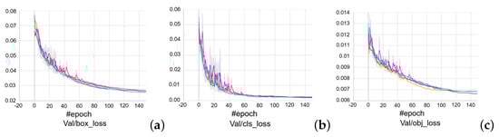
Figure 14.
Validation (a) box, (b) class, (c) object losses in 5-fold cross validation, with each different color corresponding to a fold as in Figure 12.
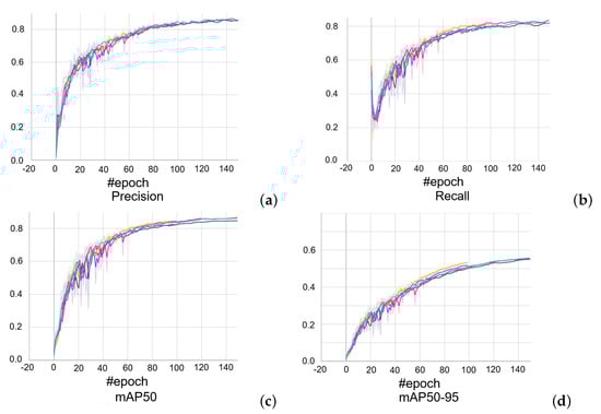
Figure 15.
Performance metrics (a) precision, (b) recall, (c) mAP50, (d) mAP50-95 across 5-fold cross validation, with each different color corresponding to a fold as in Figure 12.
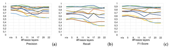
Figure 16.
Evaluation of (a) precision, (b) recall, (c) F1 score of Experiment 2 show the performance for different numbers of frozen layers with colors representing the different classes of Figure 5.
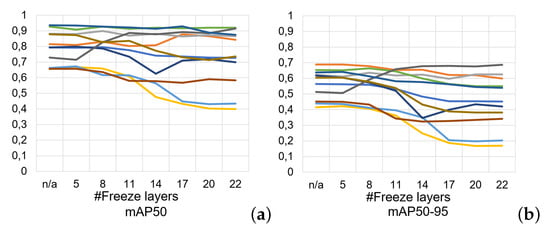
Figure 17.
Evaluation of (a) mAP50, (b) mAP50-95 metrics of Experiment 2 show the performance for different numbers of frozen layers with colors representing the different classes of Figure 5.
In terms of training losses, there is a consistent decrease across all folds, as demonstrated in Figure 13. This trend, evident in the box, object, and class losses, signifies that the model is effectively learning to minimize errors in various aspects of object detection, including the accuracy of bounding boxes, detection reliability, and classification accuracy. The validation losses across all folds show a decreasing or stable trend (Figure 14), indicating that the model is not overfitting and is capable of generalizing well to unseen data. This consistency suggests that the training of this object detection model is effectively tuned, so the parameters for training models of each experiment will be fixed to the values used for training: learning rate , batch size 32, image size , weight decay , momentum , and epoch 150 (Table 1).
In contrast to the training and validation losses, there is consistent improvement in precision, recall and mean average precision (mAP) metrics across all folds (Figure 15). Precision generally shows an upward trend, indicating that the model becomes more accurate in its predictions as training progresses. Recall, assessing the model’s ability to correctly identify all relevant instances, also improves or shows significant variability across different folds. This variability might point to a trade-off between precision and recall, a common occurrence in object detection. Both mAP50 and mAP50-95 scores in Figure 15 show consistent improvement, highlighting the model’s improving accuracy across a range of intersection over union (IoU) thresholds.
5.2. Experiment 2: Evaluating the Efficacy of Transfer Learning: Fine-Tuning YOLO Pre-Trained on Single-Class Images for Multi-Class Image Detection
Experiment 2 aimed to offer critical insights into the versatility of YOLOv5s and elucidate the impact of transfer learning and fine-tuning on its capacity to handle multi-class images (Figure 10 Right), following its initial training on single-class images. The experimental hypothesis was that the baseline model (above), pre-trained on single-class images, would, with appropriate fine-tuning, effectively adapt to and accurately classify multi-class images. By evaluating the model’s performance across different levels of layer freezing, this study aimed to determine the optimal balance between knowledge retention from the pre-trained state and adaptability to new, complex detection scenarios. Training was supported by the powerful Tesla V100-SXM2-16GB with 16151MiB available on Google Colab, ensuring that the model’s fine-tuning was both rigorous and efficient.
For training, Dataset #6, a diverse collection of 573 multi-class images, was used, along with the YOLOv5s model previously fine-tuned in Experiment 1 as the foundation. The model’s ability to transfer its learned knowledge from single-class to multi-class detection was the focal point of this phase. Validation was performed on a composite dataset—Dataset #2 (400 single-class images) and Dataset #5 (430 multi-class images)—to ensure that the model did not lose its single-class detection accuracy while gaining multi-class detection proficiency. The testing phase was aligned with that of Experiment 1, using a mixed set of single-class and multi-class images from Datasets 3 and 4. This consistency allowed for a direct comparison of the model’s performance across the experiments. The effectiveness of transfer learning was systematically assessed by freezing varying numbers of layers within the model during the training process. Starting with no frozen layers, the approach escalated through progressive levels of constraint by freezing layers from the first up to the 5th, 8th, 11th, 14th, 17th, 20th, and finally, the 22nd layer out of the total 25 layers of the model. Notably, the first 10 layers constituted the backbone of the model, which are generally responsible for extracting fundamental features from images.
Experiment 2 Results (Evaluating the Efficacy of Transfer Learning, Fine-Tuning: The Precision results (Figure 16a), suggest that while the model exhibits the highest average precision with no layers frozen, a nuanced approach to layer freezing is required to balance all performance measures effectively. The recall results in Figure 16b indicate an enhanced ability to capture true positive instances when the first eight layers are frozen, which is unexpected given that a lesser degree of freedom in the model could potentially hinder such performance. However, the F1 Score results (Figure 16c) provide further evidence to advocate for freezing eight layers, as this configuration achieves the highest average F1 Score of 0.769. This suggests that restraining the adaptability of the initial layers of the model prompts a more balanced performance, possibly by leveraging the generic features learned during pre-training and refining the model’s understanding of more dataset-specific features in the subsequent layers. While the mAP50 and mAP50-95 results, detailed in Figure 17a,b, respectively, generally favor the fully adaptable model (no layers frozen), they do not significantly deteriorate when freezing eight layers. This indicates that the model retains a substantial portion of its detection capabilities even with the imposed constraints. The stable performance in mAP metrics, combined with the highest F1 Score, underscores the efficacy of freezing eight layers in achieving a robust model that not only predicts accurately but also ensures comprehensive detection coverage. Therefore, the results of freezing eight layers in Experiment 2 will be further used for comparison analysis with other experiments.
5.3. Experiment 3: Generalizability, Bias, Fairness Exploration by Combined Single-Class and Multi-Class Training
Experiment 3 (Figure 18 Left) explored the model’s ability to generalize, i.e., achieve accurate object detection results on testing data containing diverse multi-class images, which deviate significantly from the training data. To achieve this, it uses a mixed training regimen, integrating both single-class and multi-class images. Specifically, training was conducted using single-class images from Dataset #1 and multi-class images from Dataset #6. The distribution of the instances in the training dataset is shown in Figure 19a. This approach aimed to provide the YOLOv5s model, which, as in Experiment 1, is pre-trained on the COCO dataset, with broad and heterogeneous training data, under the assumption this diversity in the training phase will contribute to a higher degree of adaptability and generalizability in the resulting model. The training was powered by the Tesla V100-SXM2-16GB with 16151MiB, accessed via Google Colab. The validation phase was consistent with that of Experiment 2, using a blend of single-class images from Dataset #2 and multi-class images from Dataset #5 to ensure that the model retained its accuracy across both image types. For testing, the same datasets as in Experiments 1 and 2 (Datasets #3 and #4) were used, for direct comparability of results and the assessment of improvements or changes in performance due to the mixed training data.
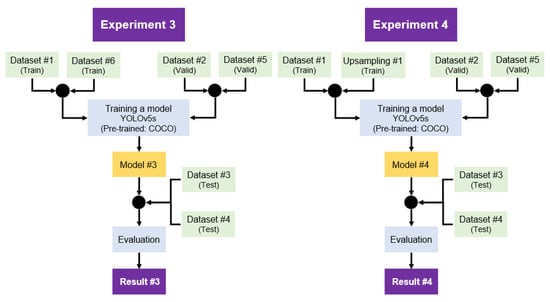
Figure 18.
Flowchart of training and evaluation. Left: Experiment 3 explores the effect of diverse multi-class training data on generalizability, fairness and bias. Right: Experiment 4 examines the effect of data augmentation on single-class images.
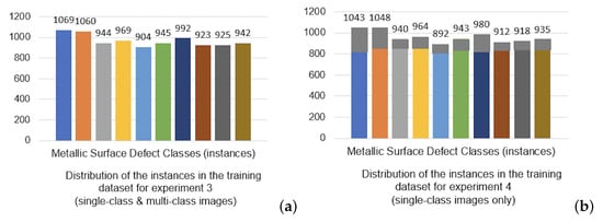
Figure 19.
Distribution of instances for metallic surface defect classes in (a) Experiments 3 and (b) 4, with the color labels shown in Figure 5.
Experiment 3 Results (Combined Single-Class and Multi-Class Training): The generalizability achieved by this training approach is evident in Table 3, which shows that Experiment 3 demonstrates a substantial improvement over Experiments 1 and 2 in terms of average precision, recall and F1 score. The detailed breakdown of results in Table 3, Table 4, Table 5 and Table 6 shows comparable or improved results per defect type. Similarly, Table 7 and Table 8 demonstrate that Experiment 3 maintains high performance in terms of its mAP50 and mAP50-95 scores across varying IoU thresholds, emphasizing its ability to generalize to accurate multi-class defect detection, while being trained on combined single and multi-class data.
Table 3.
Average precision, recall, F1 score of Experiment 1, 2, 3, 4. Experiment 3 consistently outperforms the other experimental setups.
Table 4.
Precision of Experiment 1, 2, 3, 4. Experiment 3 outperforms the others for most defect classes.
Table 5.
Recall of Experiment 1, 2, 3, 4. Experiment 3 outperforms the others for most defect classes.
Table 6.
F1 score of Experiment 1, 2, 3, 4. Experiment 3 outperforms the others for most defect classes.
Table 7.
mAP50 of Experiment 1, 2, 3, 4. Experiment 3 outperforms the others for most defect classes.
Table 8.
mAP50-95 of Experiment 1, 2, 3, 4. Experiment 3 outperforms the others for most defect classes.
Bias refers to a model’s proclivity for uneven performance across different defect types. The baseline model in Experiment 1 exhibits a high degree of bias, with significant performance fluctuations among defect types (see Appendix B). This is evident from the low precision and recall values for defects such as inclusion (In), suggesting a failure to capture the features necessary for these defect types. Contrastingly, Experiment 3’s results, depicted across Table 4 and Table 5, show minimal variation in performance across defects, indicating a reduction in bias due to the broader range of features learned from the combined single-class and multi-class images.
The assessment of fairness, i.e., the model’s equitable treatment of different defect types, reveals that Experiment 3’s approach yields a fairer model. This is particularly reflected in the F1 scores from Table 6, where the scores are not only higher on average but also display less variability across different defect types. This uniformity suggests that the combined dataset used in Experiment 3 promotes a fair learning environment where no single defect type is overly represented or neglected.
When delving into the details of individual defect types, this study observes notable trends. For instance, the precision for crease (Cr) detection consistently improves through the experiments, reaching its peak in Experiment 3, as shown in Table 4. Inclusion (In), highlighted as a challenging defect type with low scores in Experiment 1, sees marked improvement in Experiment 3 (Table 4 and Table 5), underscoring the benefits of a diverse training set. Similarly, oil spot (Os) and silk spot (Ss) defects exhibit significant improvements in Experiment 3, suggesting enhanced model capability to identify these defects accurately. One defect type, waist folding (Wf), stands out for maintaining high detection scores across all experiments, indicating certain defect features may be inherently easier for the model to learn. Also, waist folding is an isolated class shown in Figure 9. This is supported by the consistently high mAP50 and mAP50-95 scores for waist folding in Table 7 and Table 8, respectively, across all experimental setups.
5.4. Experiment 4: Evaluating the Impact of Data Augmentation on Model Performance
Experiment 4 (Figure 18 Right) was designed to test the hypothesis that a model trained on augmented single-class images could achieve performance metrics on par with or superior to those of a model trained on a naturally varied dataset. The computational backbone for the training was provided by the Tesla V100-SXM2-16 GB with MiB, facilitated through Google Colab.
Training employed an upsampled dataset derived from Dataset #1’s single-class images. The upsampling process was augmented with a series of traditional data augmentation techniques to artificially match the instance counts in Experiment 3 (Figure 19). In Figure 19b, the dark grey segments atop each bar represent the amount of instances increased through data augmentation. This method aimed to artificially induce the variety typically obtained from a mixed dataset without actually combining single and multi-class images. The validation process mirrored that of Experiments 2 and 3, employing a mixed set of single-class images from Dataset #2 and multi-class images from Dataset #5. The consistency in validation across experiments was crucial to ensure comparability of results. Testing employed Datasets #3 and #4, as with the previous experiments, to assess the augmented model’s generalization and detection capabilities across a range of scenarios.
Experiment 4 Results (Impact of Data Augmentation): Table 3 shows that, on average, Experiment 4 does not outperform the other experimental setups, except baseline Experiment 1, which only used single-class images, a trend that can be seen in more detail in Table 4, Table 5, Table 6, Table 7 and Table 8. Data augmentation in Experiment 4 matched the instance counts used in Experiment 3; however, these augmentations were not sufficient to match naturally occurring variations in data, as demonstrated by these results. They can provide a small improvement, compared to the baseline, by expanding the training dataset artificially, particularly when access to naturally varied data is constrained.
6. Generalizability, Bias Fairness
This section describes in depth how generalizability, bias reduction and fairness are assessed and achieved in the different experimental setups. It goes beyond the performance metrics of Section 5, by examining the confusion matrices for generalizability, and the fairness and bias metrics introduced in this work, focusing on the TPR, which is of interest in industrial applications. As detailed in the subsections that follow, the setup of Experiment 3 leads to improved generalizability and fairness, while reducing bias, validating our hypothesis that careful dataset management and balancing is needed to achieve such results.
6.1. Generalizability, Bias Fairness from Confusion Matrices
The confusion matrices from Experiments 1–4 can provide more insights into the generalizability, bias and fairness of these experimental setups. In terms of generalizability, the confusion matrix of Experiment 1 (Figure 20a) reveals substantial off-diagonal activity, signifying frequent misclassifications, which suggests a model with a limited capacity to generalize. Conversely, the confusion matrix from Experiment 2 (Figure 20b) exhibits improvements, as evidenced by heightened true positive rates for defects such as crescent gap and punching hole. This indicates a model with enhanced generalization abilities, although some defect types remain challenging for the model. The confusion matrix for Experiment 4 (Figure 20d) still revealed disparities in performance across defect types: although certain classes such as punching hole and waist folding were well-identified, as evidenced by high true positive rates, others like oil spot and inclusion suffered from lower accuracy and higher misclassification rates. These inconsistencies pointed to potential limitations in the model’s generalization when solely trained with augmented data. The confusion matrix from Experiment 3 (Figure 20c) demonstrates the most proficient generalization, with a significant portion of predictions correctly aligned along the diagonal, indicating a robust model that accurately identifies the majority of defect types.
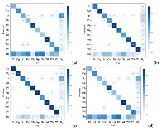
Figure 20.
Confusion matrices of Experiments 1–4 (testing set). Experiment 3 has most predictions along its diagonal, showing it most accurately identifies the majority of defects when tested on different types of data, demonstrating its improved generalizability, reduced bias and improved fairness.
In reviewing bias, the confusion matrix for Experiment 1 (Figure 20a) displays pronounced bias, with defects like waist folding being identified with high precision while oil spot and inclusion are frequently confused with other defect types. Experiment 2 (Figure 20b) shows a reduction in bias, with a more balanced prediction across defect types, albeit oil spot continues to be a problematic class. Experiment 4 (Figure 20d) exhibited a skewed performance with high false positives and negatives for specific classes, indicating a bias that could be attributed to the limitations of data augmentation in capturing the natural variance present in Experiment 3’s mixed-class training set. The confusion matrix of Experiment 3 (Figure 20c) portrays a model with the least bias, as it achieves higher accuracy across a diverse array of defect types with reduced misclassification rates.
Fairness, in this context, implies the model’s equitable performance across all defect types. The confusion matrix from Experiment 1 (Figure 20a) indicates a lack of fairness, with significant disparities in how different defects are classified—some classes are consistently misclassified as others. The matrix from Experiment 2 (Figure 20b) depicts moderate improvements in fairness, with a more balanced performance. However, certain defects, such as silk spot and water spot, are still prone to being mistaken for Background (Bg). The confusion matrix for Experiment 4 (Figure 20d) showed a lack of fairness, with certain classes being more prone to misclassification than others, suggesting that the augmented data may not provide the same level of representativeness for each class as the naturally varied dataset used in Experiment 3. In stark contrast, the confusion matrix from Experiment 3 (Figure 20c) shows a model that performs fairly across all defect types, with most classes being accurately predicted and misclassifications evenly distributed without unduly favoring or prejudicing any specific defect type.
The sequential analysis from Experiments 1 through 4 uncovers a trajectory of progressive improvement not only in terms of generalization but also in mitigating bias and enhancing fairness in classification. The confusion matrix from Experiment 3, in particular, underscores the efficacy of the combined training approach, which amalgamates single-class and multi-class images, leading to a model that is robust in its predictive accuracy and equitable across various defect types.
6.2. Fairness Measures
This study’s fairness assessment, pivotal in the domain of multi-class image predictive modeling, utilized disparate impact ratio (DIR), true positive rate differences (TPR Diff), and predictive parity difference (PPD) as metrics. To categorize data into two groups, privileged and unprivileged, the concept of class co-occurrence relationships is used. This approach identifies a strong co-occurrence between crescent gap (Cg), punching hole (Ph), and welding line (Wl) in a multi-class image dataset illustrated in Figure 9. Consequently, these defects are classified into the unprivileged group due to their frequent joint presence, which significantly influences models trained without multi-class images. Conversely, defects like crease (Cr), inclusion (In), oil spot (Os), rolled pit (Rp), silk spot (Ss), waist folding (Wf), and water spot (Ws) are assigned to the privileged group.
The disparate impact ratio (DIR), adapted to focus on the true positive rates (TPR), revealed notable differences across the experiments. The results are shown in Table 9, with the best outcomes highlighted in bold. Experiments 1 and 4 reported DIR values significantly greater than 1 (1.52 and 1.56, respectively), indicative of a model with heightened sensitivity towards the unprivileged group, which encompasses defects that co-occur frequently. Experiment 2 displayed a slight reduction in the DIR value (1.37), suggesting some mitigation of this sensitivity. However, it was Experiment 3 that presented a DIR value (1.14) closest to unity, signaling a more equitable sensitivity towards both the unprivileged and privileged groups, aligning with the objective of equal opportunity in predictive modeling.
Table 9.
Fairness measures results in Experiments 1, 2, 3, and 4 with the best outcomes shown in bold. Experiment 3 leads to the most fair and unbiased outcomes in all cases, and the same outcome for PPD as Experiment 2.
The true positive rate differences (TPR Diff) metric further underpinned these findings, with the best outcomes shown in bold fonts in Table 9. Experiments 1, 2, and 4 showed relatively high TPR Diff values (0.24, 0.26, and 0.26) from Table 9, denoting a considerable disparity in the model’s sensitivity and favoring the unprivileged group. Contrastingly, Experiment 3 achieved a significantly lower TPR Diff value (0.11), which underscored a model with a fairer distribution of sensitivity and a diminished disparity between groups.
The predictive parity difference (PPD), assessing precision equity between groups, reinforced the narrative of Experiment 3’s superior fairness. In Table 9, Experiment 1 showed the largest negative PPD value (−0.19), implying a lack of predictive parity and suggesting systematic underprediction for the privileged group. Experiments 2 and 3 demonstrated improvements, with similar lower negative PPD values (−0.08), indicating strides toward achieving predictive parity. However, Experiment 4 regressed, with a PPD value (−0.17) echoing the disparity observed in Experiment 1.
The comparative analysis of these fairness measures offers compelling evidence of Experiment 3’s balanced approach. It stands as the most equitable model, with fairness metrics suggesting a fair and unbiased prediction across the board. This analysis underscores the effectiveness of employing a naturally diverse training set, as seen in Experiment 3, which included a balanced mix of single-class and multi-class images, thus facilitating a fairer and more representative learning process. These insights are critical for the development of unbiased multi-class predictive models, particularly in high-stakes sectors where fairness is not just a metric but a mandate.
6.3. Explainability-Based Assessment of Decision-Making
We pursue explainability in our object detection framework using the Eigen Class Activation Mapping (Eigen-CAM) methodology [19,20,21] to visualize the regions within the image data that significantly inform the predictive models’ decision-making processes for our four experimental setups. By extracting 2D activations from the penultimate layer— specifically, layer number 23—of the YOLOv5s architecture, we generated heatmaps to illuminate the areas that each model attends to when distinguishing between defect types.
The Eigen-CAM visualizations for Experiment 3 (Figure 21) demonstrated a high degree of alignment with the actual defect areas, particularly in the context of multi-class images where defect classes such as inclusion and oil spot present visually similar characteristics. These heatmaps revealed distinct and precise activation regions, underscoring the model’s ability to effectively learn and discriminate between the high-level features of each class. This capacity for nuanced differentiation is indicative of a well-generalized model that has been trained on a dataset rich in both single-class and multi-class images, reflecting the diverse scenarios encountered in practical applications.
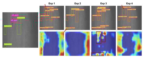
Figure 21.
Eigen-CAM results of predicting 2 similar defects in Experiments 1, 2, 3, and 4. The red square shows the captured predicted area and the red arrows denote erroneous predictions. It is clear that the model successfully focuses on the relevant areas of test images for Experiment 3, while these are largely missed by the other experimental setups.
Conversely, the heatmaps from Experiments 1, 2, and 4 (Figure 21) displayed less focused activations, occasionally overlapping or misaligned with the relevant defect areas, particularly for the similar-looking inclusion and oil spot classes. This suggests that the models from these experiments may have struggled to segregate the features of these classes effectively. Such a struggle could stem from a less robust training regimen or, in the case of Experiment 4, from potential limitations of data augmentation in adequately representing the intricate variance between defect types.
Thus, the use of Eigen-CAM can play a pivotal role in evaluating and contrasting the models’ performance across the experiments. For Experiment 3, the method corroborated the model’s discernment capabilities, affirming that the activations were indeed representative of the defects it was trained to detect. In the case of contrast, the less precise activation patterns from the other experiments pointed to a need for improved training approaches or augmentation techniques to enhance the models’ interpretability and reliability.
7. Discussion
This study embarked on an in-depth exploration of defect detection using the YOLOv5s model [13] under various experimental conditions. Through rigorous evaluation involving precision, recall, F1 scores, mAP measures [12], and fairness metrics, comprehensive insights into each model’s performance nuances were gained. Experiment 3 emerged as a frontrunner, striking a commendable balance between accuracy, generalization and fairness in predictions.
As shown and discussed in detail in Section 5 and Table 3, Table 4, Table 5, Table 6, Table 7 and Table 8, Experiment 3 outperformed the other experimental setups in most cases, in terms of precision, accuracy, recall, F1 Score and mAP. Section 5 also examines in depth specific defects that are under-represented or co-occur in single and multi-class images, providing a clear understanding of performance variations in those cases. The improved performance metrics of Section 5 confirm our hypothesis that the provision of diverse training data can allow the same model (YOLOv5s) to more accurately identify a range of defect types, appearing in both single and multi-class images in different ratios, sometimes co-occurring with other defects. Moreover, the high mAP50 and mAP50-95 scores for Experiment 3 underscore the model’s ability to maintain high accuracy across different thresholds, a key indicator of strong generalization to real-world scenarios.
Generalizability, fairness and bias are assessed in depth in Section 6 by examining confusion matrices, as well as our adapted fairness and bias metrics. Once again, the comparative analysis of the confusion matrices provides compelling evidence that the model from Experiment 3, which was trained on a combination of single-class and multi-class images, not only generalizes better to new data but also exhibits less bias and greater fairness in defect classification. This underscores the importance of appropriately using data augmentation to replicate the complex interplay of features found in a naturally varied dataset. Fairness and bias metrics are also used to quantify the fairness and bias present in each experimental setup in Section 6. These results, shown in Table 9, confirm that the setup of Experiment 3 leads to the most equitable model, resulting in the most fair outcomes, with the least bias, across the board. This analysis underscores the effectiveness of employing a naturally diverse training set, as seen in Experiment 3, which included a balanced mix of single-class and multi-class images, thus facilitating a fairer and more representative learning process. These insights are critical for the development of unbiased multi-class predictive models, particularly in high-stakes sectors where fairness is not just a metric but a mandate.
Finally, the application of Eigen-CAM for explainability demonstrated that the setup of Experiment 3 improved the model’s discernment capabilities [21]. The explainability results offered visual evidence of the model’s attentiveness to relevant features for accurate defect detection, especially for challenging classes with similar appearances. This once again confirmed our approach, which does not only perform data augmentations, but also examines the co-occurrence of defects and their under-representation so as to carefully create truly balanced training datasets. As a result, the model is provided with balanced representations of all kinds of defects, enabling it to focus on the relevant areas of defect images in order to classify them, improving its performance and reliability.
8. Conclusions and Future Work
This work emphasizes the need for ethical considerations in AI deployment, highlighting the reduction of bias and enhancement of fairness as imperatives for responsible AI application in real-world scenarios. To this end, it has introduced a strategic bias mitigation framework, aiming at the deployment of deep learning models in real-world applications in a way that ensures fair, generalizable and unbiased results. Extensive and in depth experiments using a fixed model (YOLOv5s) for consistency demonstrate that the creation of truly balanced datasets can lead to improved performance and also fairness and generalizability, while reducing bias.
The broader implications of these results are substantial and multifaceted. They underscore potential impacts on industrial quality control, the advancement of AI fairness, guidance for future AI research, influence on policy and regulation, and the shaping of public perception of AI. Our findings highlight the importance of creating truly varied and balanced datasets to train object detection models, advocating for fairer, more generalized, and interpretable AI systems. They lay the groundwork for further studies by establishing a comprehensive baseline for the performance of YOLOv5 performance in metal defect detection.
Future work could explore the effects of data balancing and augmentation, taking into account the under-representation and co-occurrence of classes in single and multi-class images, for other low-cost, high performing models, such as newer variants of YOLO (YOLOv7, YOLOv8) or others. Its aim would be to provide a comprehensive comparison of different models trained systematically according to our framework, in terms of performance and also generalizability, fairness and bias.
Author Contributions
Conceptualization, A.B.; investigation, S.R.; methodology, A.B.; software, S.R.; supervision, A.B.; validation, S.R.; writing—original draft, S.R.; writing—review and editing, A.B. All authors have read and agreed to the published version of the manuscript.
Funding
This research received no external funding.
Data Availability Statement
A public benchmarking dataset GC-10 DET was used, downloaded from https://github.com/lvxiaoming2019/GC10-DET-Metallic-Surface-Defect-Datasets?tab=readme-ov-file accessed on 30 October 2023.
Acknowledgments
This work was carried out by the authors themselves as part of their educational and research activities.
Conflicts of Interest
This work is carried out independently, with no external funding. The datasets used are public benchmarking research datasets, freely available on the web. No funders had a role in the design of the study; in the collection, analyses, or interpretation of data; in the writing of the manuscript; or in the decision to publish the results”.
Appendix A. Addressing Real-World Conditions Techniques
To effectively model the complex conditions found in industrial environments, this study employs a suite of image processing techniques aimed at replicating the variable lighting and noise interference typically encountered, described analytically in this appendix.
- Local brightness fluctuation: This method is designed to emulate localized variations in lighting, akin to the interplay of shadows or spotlights within a scene. Such fluctuations can be indicative of faulty lighting conditions, where certain regions may appear anomalously dark or bright.
where I is the original image, is the modified image, and M is a mask function that applies intensity fluctuations within the specified regions, with representing pixel coordinates.
- 2.
- Contrast adjustment in local areas: By locally manipulating the tonal range of the image, this technique can simulate differential light reception across various sections of the image, reflecting the nuanced effects of lighting on the observed subject matter.
where is the contrast adjustment factor, is the mean luminance of the local region, and I and represent the original and modified images, respectively.
- 3.
- Dodging and burning: Borrowed from traditional darkroom practices, dodging and burning are digital techniques for selectively brightening (dodging) or darkening (burning) image regions, thus mimicking the variegated effects of light exposure.
For dodging:
For burning:
where s is the effect strength, and I and are the original and modified images.
- 4.
- Linear mapping (brightness adjustment): This operation scales the pixel values across the image to adjust brightness, creating the perception that the image was captured under more or less intense light.
where f is the scaling factor for brightness adjustment.
- 5.
- Gaussian noise addition: The injection of Gaussian noise into the image serves to replicate the random intensity fluctuations that are often a byproduct of camera sensor noise.
where represents the Gaussian noise function with mean and variance .
- 6.
- Multiplicative Gaussian noise: This noise model is proportional to the image intensity, typically used to represent physical phenomena such as speckle in imaging systems.
where denotes the Gaussian noise centered around 1, indicative of no change on average.
Appendix B. Detailed Breakdown of Performance Metrics across All Folds for the Baseline Experiment 1
This appendix contains the detailed breakdown of the performance metrics across all folds, for Experiment 1, summarized in Section 5.1.
Experiment 1: 5-fold Cross Validation: Table A1, which details the precision of the model, shows that the model exhibits high precision in identifying crescent gap (Cg) and waist folding (Wf), with scores consistently above 0.94 across all five folds. However, the model struggles with inclusion (In) and silk spot (Ss), where precision is notably lower. This indicates a higher rate of false positives for these defect types.
Table A1.
Precision result of validation in 5-fold cross validation.
Table A1.
Precision result of validation in 5-fold cross validation.
| Defect Types | Fold-1 | Fold-2 | Fold-3 | Fold-4 | Fold-5 |
|---|---|---|---|---|---|
| Cr | 0.963 | 0.938 | 0.944 | 0.93 | 0.939 |
| Cg | 0.981 | 0.979 | 0.983 | 0.97 | 0.988 |
| In | 0.602 | 0.648 | 0.688 | 0.578 | 0.532 |
| Os | 0.76 | 0.746 | 0.788 | 0.739 | 0.765 |
| Ph | 0.905 | 0.863 | 0.906 | 0.87 | 0.869 |
| Rp | 0.889 | 0.95 | 0.903 | 0.913 | 0.955 |
| Ss | 0.8 | 0.738 | 0.638 | 0.767 | 0.715 |
| Wf | 0.983 | 0.95 | 0.952 | 0.944 | 0.944 |
| Ws | 0.908 | 0.882 | 0.913 | 0.835 | 0.874 |
| Wl | 0.963 | 0.915 | 0.876 | 0.844 | 0.796 |
| Average | 0.875 | 0.861 | 0.859 | 0.839 | 0.838 |
Table A2 shows the model demonstrates commendable performance in detecting crease (Cr), crescent gap (Cg), and welding line (Wl), with most recall rates being above 0.9. The lower recall rates for inclusion (In) and silk spot (Ss) indicate that the model tends to miss a significant number of these defects, which is a concern for overall detection reliability. The recall rates are slightly lower than precision rates, with averages ranging from 0.796 to 0.835, pointing to a potential area for improvement in the model’s ability to detect all relevant instances.
Table A2.
Recall result of validation in 5-fold cross validation.
Table A2.
Recall result of validation in 5-fold cross validation.
| Defect Types | Fold-1 | Fold-2 | Fold-3 | Fold-4 | Fold-5 |
|---|---|---|---|---|---|
| Cr | 0.972 | 0.922 | 0.932 | 0.9 | 0.924 |
| Cg | 0.963 | 0.942 | 0.949 | 0.975 | 0.966 |
| In | 0.651 | 0.599 | 0.656 | 0.561 | 0.519 |
| Os | 0.717 | 0.698 | 0.715 | 0.684 | 0.693 |
| Ph | 0.793 | 0.826 | 0.879 | 0.824 | 0.839 |
| Rp | 0.891 | 0.928 | 0.986 | 0.94 | 0.887 |
| Ss | 0.571 | 0.601 | 0.535 | 0.549 | 0.519 |
| Wf | 0.892 | 0.85 | 0.877 | 0.859 | 0.853 |
| Ws | 0.874 | 0.878 | 0.873 | 0.845 | 0.839 |
| Wl | 0.953 | 0.925 | 0.951 | 0.938 | 0.925 |
| Average | 0.828 | 0.817 | 0.835 | 0.808 | 0.796 |
The F1 score results in Table A3 demonstrate strong performance in detecting crescent gap (Cg) and waist folding (Wf), with F1 scores consistently high across all folds, particularly notable for Cg with scores above 0.96. In contrast, the model struggles with inclusion (In) and silk spot (Ss), indicated by their notably lower F1 scores, aligning with the trends observed in precision and recall. Other defect types like crease (Cr), welding line (Wl), oil spot (Os), punching hole (Ph), and rolled pit (Rp) show moderate performance with some variability across folds. The average F1 scores, ranging from 0.816 to 0.851, suggest a relatively consistent performance across different data subsets, though with a slight decline in later folds. This table reinforces the findings from previous tables, highlighting the model’s strengths in certain defect types and underscoring areas needing improvement, particularly for defects where both precision and recall are lower.
Table A3.
F1 score result of validation in 5-fold cross validation.
Table A3.
F1 score result of validation in 5-fold cross validation.
| Defect Types | Fold-1 | Fold-2 | Fold-3 | Fold-4 | Fold-5 |
|---|---|---|---|---|---|
| Cr | 0.967 | 0.93 | 0.938 | 0.915 | 0.931 |
| Cg | 0.972 | 0.96 | 0.966 | 0.972 | 0.977 |
| In | 0.626 | 0.623 | 0.672 | 0.569 | 0.525 |
| Os | 0.738 | 0.721 | 0.75 | 0.71 | 0.727 |
| Ph | 0.845 | 0.844 | 0.892 | 0.846 | 0.854 |
| Rp | 0.89 | 0.939 | 0.943 | 0.926 | 0.92 |
| Ss | 0.666 | 0.662 | 0.582 | 0.64 | 0.601 |
| Wf | 0.935 | 0.897 | 0.913 | 0.899 | 0.896 |
| Ws | 0.891 | 0.88 | 0.893 | 0.84 | 0.856 |
| Wl | 0.958 | 0.92 | 0.912 | 0.889 | 0.856 |
| Average | 0.851 | 0.838 | 0.847 | 0.823 | 0.816 |
Table A4 presents the model’s performance in terms of mAP50, which is a crucial metric in object detection. Here, the model again shows high scores in detecting crescent gap (Cg), waist folding (Wf), and welding line (Wl), consistent with the high precision and recall rates observed earlier. The lower mAP50 scores for inclusion (In) and silk spot (Ss) reinforce the challenges faced by the model in accurately identifying these defect types. Notably, the average mAP50 demonstrates consistency from folds 1 to 5, which implies that the model can generalize well across different data samples within the same dataset.
Table A4.
mAP50 result of validation in 5-fold cross validation.
Table A4.
mAP50 result of validation in 5-fold cross validation.
| Defect Types | Fold-1 | Fold-2 | Fold-3 | Fold-4 | Fold-5 |
|---|---|---|---|---|---|
| Cr | 0.967 | 0.954 | 0.97 | 0.944 | 0.954 |
| Cg | 0.984 | 0.969 | 0.983 | 0.979 | 0.98 |
| In | 0.601 | 0.613 | 0.696 | 0.571 | 0.478 |
| Os | 0.746 | 0.745 | 0.765 | 0.759 | 0.745 |
| Ph | 0.819 | 0.859 | 0.896 | 0.824 | 0.871 |
| Rp | 0.934 | 0.964 | 0.989 | 0.961 | 0.94 |
| Ss | 0.647 | 0.688 | 0.563 | 0.69 | 0.606 |
| Wf | 0.972 | 0.952 | 0.958 | 0.943 | 0.935 |
| Ws | 0.915 | 0.916 | 0.906 | 0.886 | 0.875 |
| Wl | 0.968 | 0.958 | 0.943 | 0.907 | 0.902 |
| Average | 0.855 | 0.862 | 0.867 | 0.846 | 0.829 |
Table A5 sheds light on the model’s performance across a range of IoU thresholds (mAP50-95). The scores here are generally lower than those for mAP50, reflecting the increased difficulty of maintaining high precision at higher IoU thresholds. The model’s performance on inclusion (In) and silk spot (Ss) is particularly affected at these stricter thresholds, with significantly lower scores. The overall lower mAP50-95 scores across all defect types suggest that the model may struggle to maintain high precision when stricter criteria for defect detection are applied.
Table A5.
mAP50-95 result of validation in 5-fold cross validation.
Table A5.
mAP50-95 result of validation in 5-fold cross validation.
| Defect Types | Fold-1 | Fold-2 | Fold-3 | Fold-4 | Fold-5 |
|---|---|---|---|---|---|
| Cr | 0.744 | 0.716 | 0.711 | 0.685 | 0.686 |
| Cg | 0.744 | 0.737 | 0.722 | 0.682 | 0.715 |
| In | 0.274 | 0.236 | 0.287 | 0.241 | 0.194 |
| Os | 0.399 | 0.364 | 0.365 | 0.347 | 0.332 |
| Ph | 0.581 | 0.590 | 0.616 | 0.570 | 0.560 |
| Rp | 0.724 | 0.701 | 0.732 | 0.715 | 0.684 |
| Ss | 0.264 | 0.310 | 0.215 | 0.309 | 0.271 |
| Wf | 0.704 | 0.674 | 0.689 | 0.635 | 0.605 |
| Ws | 0.603 | 0.605 | 0.592 | 0.550 | 0.557 |
| Wl | 0.694 | 0.653 | 0.607 | 0.605 | 0.586 |
| Average | 0.573 | 0.559 | 0.554 | 0.534 | 0.519 |
The analysis of the YOLOv5s model’s performance shows that this model, trained on a substantial dataset of 5760 images, demonstrates significant capabilities in certain aspects, while also highlighting potential limitations that could be addressed for enhanced performance. One of the standout observations is the model’s robust ability to detect specific types of defects, notably crescent gap (Cg) and waist folding (Wf). These defect types consistently show high precision, recall, and F1 scores across all folds in the cross-validation process. Such performance suggests that the model has effectively learned to identify the distinguishing features of these defects, possibly due to their distinct characteristics or adequate representation in the training set. Other defects like crease (Cr) and welding line (Wl) also exhibit commendable detection rates, although they display some variability across different folds.
However, the model faces challenges with certain defects, particularly inclusion (In) and silk spot (Ss). These types consistently score lower across all evaluation metrics, indicating difficulties in accurately detecting them. This could be attributed to the complexity of these defects, their resemblance to non-defective areas, similarities with the background, variability within the class, or difficulty in distinguishing this class from others, or extremely small scale illustrated in Figure 11. The variable performance with defects like oil spot (Os), punching hole (Ph), and rolled pit (Rp) further suggests that while the model is capable of detecting these defects to a certain extent, there is notable room for improvement.
The consistency in the model’s performance, despite a slight decline in average scores across different folds (especially in F1 scores), indicates a general robustness. This suggests that the model’s effectiveness is not overly sensitive to specific data partitions, a crucial aspect for practical applications. However, the observed variability points to potential differences in the difficulty of detecting certain defects in different data subsets, highlighting the importance of a well-rounded and diverse training dataset. An important insight from this analysis is the need for a balance between precision and recall, which varies across defect types. In some cases, higher precision coupled with lower recall suggests a cautious approach by the model, potentially leading to missed defects. On the other hand, higher recall than precision in certain defects could imply over-identification, resulting in false positives. The model’s lower performance in mAP50-95 compared to mAP50 across defect types is indicative of a decline in accuracy at stricter IoU thresholds. This highlights a need for enhancing the model’s robustness and precision, especially in more challenging detection scenarios.
References
- Harvey, C. U.S. Product Recalls Hit Four-Year High in First Quarter of 2023. 2023. Available online: https://www.prnewswire.com/news-releases/us-product-recalls-hit-four-year-high-in-first-quarter-of-2023-301834964.html (accessed on 6 November 2023).
- See, J.E.; Drury, C.G.; Speed, A.; Williams, A.; Khalandi, N. The role of visual inspection in the 21st century. Proc. Hum. Factors Ergon. Soc. Annu. Meet. 2017, 61, 262–266. [Google Scholar] [CrossRef]
- Lv, X.; Duan, F.; Jiang, J.; Fu, X.; Gan, L. Deep metallic surface defect detection: The new benchmark and detection network. Sensors 2020, 20, 1562. [Google Scholar] [CrossRef] [PubMed]
- Wang, Y.; Wang, H.; Xin, Z. Efficient detection model of steel strip surface defects based on YOLO-V7. IEEE Access 2022, 10, 133936–133944. [Google Scholar] [CrossRef]
- Wang, K.; Teng, Z.; Zou, T. Metal defect detection based on YOLOv5. J. Phys. Conf. Ser. 2022, 2218, 012050. [Google Scholar] [CrossRef]
- Akhyar, F.; Liu, Y.; Hsu, C.Y.; Shih, T.K.; Lin, C.Y. FDD: A deep learning–based steel defect detectors. Int. J. Adv. Manuf. Technol. 2023, 126, 1093–1107. [Google Scholar] [CrossRef] [PubMed]
- Zhang, Y.; Shu, S.; Lang, X.; Liang, H.; Yu, Z.; Yang, Z. A real-time method for detecting bottom defects of lithium batteries based on an improved YOLOv5 model. Meas. Sci. Technol. 2023, 34, 125149. [Google Scholar] [CrossRef]
- Zhou, C.; Lu, Z.; Lv, Z.; Meng, M.; Tan, Y.; Xia, K.; Liu, K.; Zuo, H. Metal surface defect detection based on improved YOLOv5. Sci. Rep. 2023, 13, 20803. [Google Scholar] [CrossRef] [PubMed]
- Wang, L.; Liu, X.; Ma, J.; Su, W.; Li, H. Real-Time Steel Surface Defect Detection with Improved Multi-Scale YOLO-v5. Processes 2023, 11, 1357. [Google Scholar] [CrossRef]
- Mehta, M. AFF-YOLO: A Real-time Industrial Defect Detection method based on Attention Mechanism and Feature Fusion. 2023. Available online: https://www.researchsquare.com/article/rs-3449230/v1 (accessed on 13 November 2023).
- Liu, P.; Su, S.; Gao, X.; Zheng, H.; Ma, Z. Defect detection for mechanical design products with faster r-cnn network. Math. Probl. Eng. 2022, 2022, 3209721. [Google Scholar] [CrossRef]
- Ren, S.; He, K.; Girshick, R.; Sun, J. Faster R-CNN: Towards Real-Time Object Detection with Region Proposal Networks. In Proceedings of the Advances in Neural Information Processing Systems, Montreal, QC, Canada, 7–12 December 2015; pp. 91–99. [Google Scholar]
- Jocher, G.; Waxman, S. Comprehensive Guide to Ultralytics YOLOv5. 2023. Available online: https://docs.ultralytics.com/yolov5/#explore-and-learn (accessed on 13 November 2023).
- Bellamy, R.K.; Dey, K.; Hind, M.; Hoffman, S.C.; Houde, S.; Kannan, K.; Lohia, P.; Martino, J.; Mehta, S.; Mojsilovic, A.; et al. AI Fairness 360: An extensible toolkit for detecting, understanding, and mitigating unwanted algorithmic bias. arXiv 2018, arXiv:1810.01943. [Google Scholar]
- Barocas, S.; Selbst, A.D. Big data’s disparate impact. Calif. Law Rev. 2016, 104, 671–732. [Google Scholar] [CrossRef]
- Hardt, M.; Price, E.; Srebro, N. Equality of opportunity in supervised learning. In Proceedings of the Advances in Neural Information Processing Systems, Barcelona, Spain, 5–10 December 2016; Volume 29. [Google Scholar]
- Kleinberg, J.; Mullainathan, S.; Raghavan, M. Inherent trade-offs in the fair determination of risk scores. arXiv 2016, arXiv:1609.05807. [Google Scholar]
- Selbst, A.D.; Boyd, D.; Friedler, S.A.; Venkatasubramanian, S.; Vertesi, J. Fairness and Abstraction in Sociotechnical Systems. In Proceedings of the Conference on Fairness, Accountability, and Transparency, Atlanta, GA, USA, 29–31 January 2019; pp. 59–68. [Google Scholar]
- Muhammad, M.B.; Yeasin, M. Eigen-cam: Class activation map using principal components. In Proceedings of the 2020 International Joint Conference on Neural Networks (IJCNN), Glasgow, UK, 19–24 July 2020; pp. 1–7. [Google Scholar]
- Selvaraju, R.R.; Cogswell, M.; Das, A.; Vedantam, R.; Parikh, D.; Batra, D. Grad-CAM: Visual Explanations from Deep Networks via Gradient-Based Localization. In Proceedings of the IEEE International Conference on Computer Vision, Venice, Italy, 22–29 October 2017; pp. 618–626. [Google Scholar]
- Szegedy, C.; Liu, W.; Jia, Y.; Sermanet, P.; Reed, S.; Anguelov, D.; Erhan, D.; Vanhoucke, V.; Rabinovich, A. Going deeper with convolutions. In Proceedings of the IEEE Conference on Computer Vision and Pattern Recognition (CVPR), Boston, MA, USA, 7–12 June 2015; pp. 1–9. [Google Scholar]
Disclaimer/Publisher’s Note: The statements, opinions and data contained in all publications are solely those of the individual author(s) and contributor(s) and not of MDPI and/or the editor(s). MDPI and/or the editor(s) disclaim responsibility for any injury to people or property resulting from any ideas, methods, instructions or products referred to in the content. |
© 2024 by the authors. Licensee MDPI, Basel, Switzerland. This article is an open access article distributed under the terms and conditions of the Creative Commons Attribution (CC BY) license (https://creativecommons.org/licenses/by/4.0/).