Deep Reinforcement Learning-Based Process Control in Biodiesel Production

Abstract

The control of complex industrial processes has been a forefront research topic. Biodiesel production, as a typical complex industrial reaction process, exhibits multivariable coupling, nonlinearity, and high latency, making it challenging for traditional control methods to achieve real-time control under varying operating conditions. To address this issue, this paper proposes a control method based on the twin delayed deep deterministic policy gradient (TD3) algorithm, which dynamically adjusts process parameters to achieve the adaptive optimization control of complex processes. A simplified biodiesel production process model was established to simulate the actual production process. Subsequently, a controller based on the TD3 algorithm was designed and implemented for this model. To evaluate the performance of the proposed controller, comparative experiments were conducted with traditional controllers and deep deterministic policy gradient (DDPG) controllers. The effects of different control strategies were analyzed through simulation experiments. The results demonstrate that the proposed controller achieves the objectives while exhibiting a lower overshoot and shorter settling time and fully validates the effectiveness of the proposed control strategy in terms of both the dynamic and steady-state performance in the production process.

1. Introduction

Traditional diesel fuel, widely used in transportation, power generation, and industrial applications, has significant negative impacts on climate change and human health due to particulate matter and nitrogen oxide (NOx) emissions [1]. As traditional fossil fuels become scarce and environmental concerns grow, biodiesel, a sustainable and renewable alternative fuel, has attracted increasing attention. Produced from vegetable oils and animal fats, biodiesel exhibits the characteristics of biodegradability, low toxicity, and lower emissions, mitigating the environmental problems associated with fossil fuels [2].

In biodiesel production, the final yield is a critical control variable that is intricately coupled with other process variables such as feed flow rate, feed concentration, and feed temperature [3]. In most industrial processes, the setpoints of crude oil flow rate and catalyst flow rate are adjusted based on existing production and research experience to indirectly track the desired final yield. However, due to the nonlinearity, high latency, and multivariable nature of biodiesel production, empirical settings often fail to maintain a stable yield, leading to product quality degradation and increased production costs. Therefore, in-depth research on this production process and the design of efficient process control strategies are of great significance for improving biodiesel yield, reducing energy consumption, and minimizing waste [4].

Traditional control methods for biodiesel production, including fuzzy control [5,6] and model predictive control (MPC) [7], have been widely studied. For instance, Manimaran et al. [8] proposed an MPC-based method for controlling the transesterification process, optimizing controller parameters using genetic algorithms. Gupta et al. [9] employed a two-layer control framework combining constrained iterative learning control and explicit MPC to address yield fluctuations under disturbances. However, due to the fixed parameters and lack of adaptability, traditional methods struggle to handle the complex and dynamic nature of biodiesel production, limiting the achievable yield. Deep reinforcement learning, capable of learning system dynamics through continuous interaction with the environment and adapting to varying reaction conditions, offers a promising solution for such complex systems.

Mnih et al. [10] introduced the deep Q-network (DQN) algorithm, which combined deep neural networks with reinforcement learning. By using convolutional neural networks to approximate the Q-function, DQN achieved human-level performance in a variety of Atari games with discrete action spaces. Lillicrap et al. [11] proposed the deep deterministic policy gradient (DDPG) algorithm, which extended the action space of DQN to continuous domains by incorporating techniques such as experience replay and target Q-networks to enhance stability. Building upon the actor–critic framework, Fujimoto et al. [12] introduced the twin delayed deep deterministic policy gradient (TD3) algorithm, comprising an actor network, two critic networks, and their respective target networks. The critic networks learn the Q-function, while the actor network updates the policy $\pi$ under the guidance of the critic. The training process involves optimizing the parameters of the actor, critic, and target networks, with delayed updates for improved stability. Compared to earlier reinforcement learning algorithms, TD3 has demonstrated significant advantages in complex industrial control tasks.

In recent years, deep reinforcement learning algorithms have shown great promise in addressing process control challenges. Powell et al. [13] proposed a reinforcement learning-based real-time optimization method, embedding optimal decisions in a neural network for steady-state optimization and employing hybrid training to enhance real-time processing capabilities. Peng et al. [14] combined PID control with the deep deterministic policy gradient (DDPG) algorithm to address the low-power level water level control problem in nuclear power plants, highlighting the feasibility and effectiveness of deep reinforcement learning-based control methods in industrial applications. Panjapornpon et al. [15] applied a DDPG-based control method to handle pH and liquid level control in a CSTR, demonstrating superior tracking speed and stability compared to traditional controllers. Chowdhury et al. [16] employed entropy maximization to improve the twin delayed deep deterministic policy gradient (TD3) algorithm for PID tuning, demonstrating its effectiveness in controlling the temperature and feed flow rate of a continuous stirred-tank reactor (CSTR). However, these studies have primarily focused on applying deep reinforcement learning algorithms to simplified chemical processes, while their application to complex processes like biodiesel production remains underexplored. In biodiesel production, the coupling relationships between variables are complex and dynamic, making it challenging for traditional control methods to achieve optimal performance. Deep reinforcement learning algorithms, capable of learning from historical data and system states, can make optimal control decisions, leading to more efficient production.

In this paper, a deep reinforcement learning (TD3) algorithm is proposed for controlling biodiesel production. Firstly, a TD3 algorithm controller was designed based on the dynamic model of biodiesel production. Subsequently, a deep reinforcement learning environment and reward function are constructed using the model and a neural network. After training, an optimized control policy is obtained. Finally, simulation experiments are conducted to compare the tracking performance of the proposed method with traditional control algorithms and other reinforcement learning algorithms.

2. Physical System

To evaluate advanced fault detection and diagnosis methods and control and optimization strategies, the benchmark model BDsim [17] is employed. The model is capable of the following:

Simulating the impact of critical process variables, including temperature and catalyst flow rate, on product yield. Additionally, the model enables dynamic simulations to validate the performance of the TD3 control algorithm. Biodiesel production, involving the transesterification of oil and methanol, consists of a reactor, separator, washer, and dryer, as illustrated in Figure 1. The experiment is based on the following assumptions:

(1)

The raw materials are natural products with constant composition;

(2)

The catalyst concentration is assumed to be constant throughout the reaction;

(3)

Any side reactions, such as saponification, are neglected.

Raw materials and methanol are fed into the reactor, where they are thoroughly mixed through agitation. Under specific temperature conditions and in the presence of a basic catalyst, the triglycerides (TG) react with methanol (M) via transesterification to produce fatty acid esters (E) and glycerol (G) as a byproduct. The reaction can be represented as follows:

$$\begin{array}{l}\mathrm{TG}+\mathrm{M}\underset{{\mathrm{k}}_2}{\overset{{\mathrm{k}}_1}{\rightleftarrows }}\mathrm{DG}+\mathrm{E}\\ \mathrm{DG}+\mathrm{M}\underset{{\mathrm{k}}_4}{\overset{{\mathrm{k}}_3}{\rightleftarrows }}\mathrm{MG}+\mathrm{E}\\ \mathrm{MG}+\mathrm{M}\underset{{\mathrm{k}}_6}{\overset{{\mathrm{k}}_5}{\rightleftarrows }}\mathrm{G}+\mathrm{E}\end{array}$$

where TG, DG, MG, M, E, and G represent triglycerides, diglycerides, monoglycerides, methanol, ester, and glycerol, respectively. Due to the incomplete nature of the reaction, the mixture leaving the reactor contains not only the desired products but also a small amount of unreacted materials. Therefore, the mixture must be separated. To facilitate the separation process, the mixture is first cooled in a heat exchanger before entering the separator unit. A gravity settling is then employed to separate the immiscible glycerol (G) and ester (E). In the separator, the mixture separates into two phases: the denser G settles at the bottom as the heavy phase, while the lighter E separates into the upper light phase. The overflowed light phase is collected and sent to a washer, where it is washed with water to remove methanol, catalyst, and other residual impurities. The final product, commercial biodiesel, has a minimum purity of 96.5% [18].

2.1. Reactor

For the simplicity of the model equations, the set is defined as a collection of chemical species, denoted as $\mathrm{I}=\left\{\mathrm{TG},\mathrm{DG},\mathrm{MG},\mathrm{M},\mathrm{E},\mathrm{G}\right\}$. Starting from the material and energy balances, the differential equations for the reactor can be represented by Equations (1) and (2):

$$n_{\mathrm{R}}{\displaystyle \frac{\mathrm{d}{x}_{\mathrm{R},i}}{ \mathrm{d}t}}=F_{\mathrm{o}}\left(x_{\mathrm{o},i}-x_{\mathrm{R},i}\right)+F_{\mathrm{m}}\left(x_{\mathrm{m},i}-x_{\mathrm{R},i}\right)+r_i{V}_{\mathrm{R}}(i\in \mathrm{I})$$

(1)

$$n_{\mathrm{R}}{c}_{\mathrm{p},\mathrm{R}}^{*}{\displaystyle \frac{\mathrm{d}{T}_{\mathrm{R}}}{\mathrm{d}t}}=F_{\mathrm{o}}{c}_{\mathrm{p},\mathrm{o}}^{*}\left(T_{\mathrm{o}}-T_{\mathrm{R}}\right)+F_{\mathrm{m}}{c}_{\mathrm{p},\mathrm{m}}^{*}\left(T_{\mathrm{m}}-T_{\mathrm{R}}\right)+{\displaystyle \sum _{j=1}^3{\left(-\Delta H_{\mathrm{r}}\right)}_j}{r}_j{V}_{\mathrm{R}}$$

(2)

with the total amount of substance inside the reactor given by

$$n_{\mathrm{R}}=V_{\mathrm{R}}·({\displaystyle \sum _{i\in I}\frac{M_i}{{\rho }_i}}{x}_{\mathrm{R},i})$$

where $x_{R,i}$ represents the concentrations of various species in the reactor, $F_M, F_O$ are the flow rates of methanol and oil, $r$ is the reaction rates of the different components, $V_R$ is the volume of the reactor, $T_R$ is the reactor temperature, $T_M, T_O$ are the temperatures of methanol and inlet oil, respectively, and $c_{\mathrm{p},}^{*}$,$\Delta H_{\mathrm{r}}$ are the specific heat capacity and heat of reaction, respectively. The specific values for these parameters can be found in [18].

Finally, the molar flow rate leaving the reactor unit is obtained by

$$N_{\mathrm{R}}={\displaystyle \frac{M_{\mathrm{o}}{F}_{\mathrm{o}}+M_{\mathrm{m}}{F}_{\mathrm{m}}}{M_{\mathrm{R}}}}-{\displaystyle \frac{V_{\mathrm{R}}{\displaystyle \sum _{i\in \mathrm{I}}{M}_i}\frac{\mathrm{d}{x}_{\mathrm{R},i}}{ \mathrm{d}t}}{M_{\mathrm{R}}{\displaystyle \sum _{i\in \mathrm{I}}\frac{M_i}{{\rho }_i}}{x}_{\mathrm{R},i}}}+{\displaystyle \frac{V_{\mathrm{R}}{\displaystyle \sum _{i\in \mathrm{I}}\frac{M_i}{{\rho }_i}}\frac{\mathrm{d}{x}_{\mathrm{R},i}}{ \mathrm{d}t}}{{\left({\displaystyle \sum _{i\in \mathrm{I}}\frac{M_i}{{\rho }_i}}{x}_{\mathrm{R},i}\right)}^2}}$$

The numerical values of the parameters are provided in Appendix A.

2.2. Heat Exchanger

The heat exchanger reduces the temperature of the reaction mixture to the desired separation temperature by releasing energy. Since no reaction occurs within the heat exchanger, the outlet stream has the same composition as the inlet stream, as shown in Equation (3). $Q$ represents the heat removed in the heat exchanger.

$$T_{\mathrm{heat}}=T_{\mathrm{R}}-{\displaystyle \frac{Q_{\mathrm{heat}}}{N_{\mathrm{R}}{c}_{\mathrm{p},\mathrm{R}}^{*}}}$$

(3)

2.3. Decanter

From the molar mass balance of the light and heavy phases, equations for the compositions of the light- and heavy-phase mixtures in the separator are obtained. The specific expressions are as shown in Equations (4) and (5):

$$n_{\mathrm{L}}{\displaystyle \frac{\mathrm{d}{x}_{\mathrm{L},i}}{ \mathrm{d}t}}=\left({\displaystyle \frac{{\xi }_i}{{\displaystyle \sum _{k\in \mathrm{I}}\left({\xi }_k{x}_{\mathrm{R},k}\right)}}}{x}_{\mathrm{R},i}-x_{\mathrm{L},i}\right){\displaystyle \sum _{k\in 1}\left({\xi }_k{x}_{\mathrm{R},k}\right)}{N}_{\mathrm{R}}(i\in \mathrm{I})$$

(4)

$$n_{\mathrm{H}}{\displaystyle \frac{\mathrm{d}{x}_{\mathrm{H},i}}{ \mathrm{d}t}}=\left({\displaystyle \frac{1-{\xi }_i}{{\displaystyle \sum _{k\in \mathrm{I}}\left(\left(1-{\xi }_k\right)x_{\mathrm{R},\mathrm{k}}\right)}}}{x}_{\mathrm{R},i}-x_{\mathrm{H},i}\right){\displaystyle \sum _{k\in \mathrm{I}}\left(\left(1-{\xi }_k\right)x_{\mathrm{R},k}\right)}{N}_{\mathrm{R}}(i\in \mathrm{I}\backslash \{\mathrm{TG},\mathrm{DG},\mathrm{MG}\})$$

(5)

where $x_{\mathrm{L},i}$ represents the concentrations of various species in the light phase, $x_{\mathrm{H},i}$ in the heavy phase, $N_R$ is the flow rate of the mixture leaving the reactor, $n$ is the molar amount of the mixture, and $\xi$ is the split fraction, the ratio of the concentration of each substance in the light phase to that before separation. The mixture entering the separator is split asymmetrically. Due to the strong affinity between TG, DG, MG, and esters, all triglycerides are separated into the light phase with a split fraction of $\xi$ set to 1. Glycerol (G) and part of the methanol (M) are separated into the heavy phase. The overflow of the light phase over the baffle maintains a constant total liquid height $h_D$ within the separator, where $h_{\mathrm{L}}$ is the height of the light phase. The height of the light phase is as shown in Equation (6).

$$h_{\mathrm{L}}=h_{\mathrm{D}}-h_{\mathrm{H}}$$

(6)

The height of the heavy phase, $h_{\mathrm{H}}$, is calculated by the following equation (7):

$${\mathrm{A}}_{\mathrm{D}}{h}_{\mathrm{H}}=n_{\mathrm{H}}{\displaystyle \sum _{k\in \mathrm{I}}\left(x_{\mathrm{H},k}\frac{M_k}{{\rho }_k}\right)}$$

(7)

In the equation, ${\mathrm{A}}_{\mathrm{D}}$ denotes the cross-sectional area of the separator.

Assuming an ideal environment where heat exchange between the mixture inside the separator and the surroundings is negligible, the expression for the separator temperature $T_{\mathrm{D}}$ is derived based on the energy balance equation, as shown in Equation (8).

$$\left(n_{\mathrm{L}}{c}_{\mathrm{p},\mathrm{L}}^{*}+n_{\mathrm{H}}{c}_{\mathrm{p},\mathrm{H}}^{*}\right){\displaystyle \frac{\mathrm{d}{T}_{\mathrm{D}}}{\mathrm{d}t}}=N_{\mathrm{R}}{c}_{\mathrm{p},\mathrm{R}}^{*}\left(T_{\mathrm{heat}}-T_{\mathrm{D}}\right)$$

(8)

2.4. Washer + Dryer

In industrial processes, unpurified biodiesel produced from separation may contain residual methanol, glycerol, and sodium salts. Since these impurities are water soluble, washing and drying steps are employed to remove them, leaving only E and residual TG, DG, and MG. Therefore, the formula for the final yield of biodiesel is as shown in Equation (9):

$$y\text{'}={\displaystyle \frac{x_i^{\prime }{M}_i}{{\displaystyle \sum _{j\in \mathrm{I}\text{}(\mathrm{M},\mathrm{G}\}}{x}_j^{\prime }}{M}_j}}={\displaystyle \frac{x_{\mathrm{L},i}{M}_i}{{\displaystyle \sum _{j\in \mathrm{I}\text{}\{\mathrm{M},\mathrm{G}\}}{x}_{\mathrm{L},j}}{M}_j}}(i\in \mathrm{I}\backslash \{\mathrm{M},\mathrm{G}\})$$

(9)

where $x_i$ denotes the mole fraction of the mixture, $M$ is the molar mass, and $y\text{'}$ represents the final yield. Both excessively high and low reaction temperatures can significantly affect the reaction rate and final yield. Therefore, variables $T_R$ and $y\text{'}$ are chosen as the controlled variables in this paper. Multiple variables in the reaction process, such as temperature and flow rate, are highly coupled. Considering these interactions, oil temperature $To$, methanol flow rate $F_m$, and oil flow rate $F_{\mathrm{o}}$ are selected as the manipulated variables.

3. Controller Design

3.1. Markov Decision Process

Reinforcement learning studies the interactions between an agent and an environment, where the agent learns an optimal policy to make sequential decisions and maximize a cumulative reward [19]. The reinforcement learning problem is typically modeled as a Markov decision process (MDP), defined by a tuple $(S,A,p,r)$, where $S$ is the state space, $A$ is the action space, $p(s_{t+1}|s_t,a_t)$ is the state transition probability, and $r(s_t,a_t)$ is the reward function. At each time step t, the agent selects an action $a_t$ in state $s_t$ according to its policy $\pi$ and receives a reward $r$ and transitions to a new state $s_{t+1}$ based on the transition probability [20]. This process continues until the environment terminates, as illustrated in Figure 2.

The agent’s actions are determined by the policy $\pi : S\to P(A)$, where $P(A)$ is a probability distribution over the action space. For stochastic policies, $\pi (a_t|s_t)$ defines the probability of selecting action $At$ given state $St$.

The value of policy $\pi$ for the action taken in state S_t is evaluated through the Q-value function $Q^{\pi }:S\times A\to ℝ$. In Equation (10), $Q^{\pi }\left(s_t,a_t\right)$ represents the expected cumulative return starting from state $s$, after executing action a and then using a specific policy $\pi$. This is referred to as the state-action value function. In Equation (11), $V^{\pi }\left(s_t\right)$ represents the expected cumulative return starting from state $s$ while following policy π, which is referred to as the state value function.

$$Q^{\pi }\left(s_t,a_t\right)={\mathbb{E}}_{\pi }\left[{\displaystyle \sum _{t=0}^{\infty }{\gamma }^t}r\left(s_t,a_t\right)|s=s_t,a=a_t\right]$$

(10)

$$V^{\pi }\left(s_t\right)={\mathbb{E}}_{\pi }\left[{\displaystyle \sum _{t=0}^{\infty }{\gamma }^t}r\left(s_t,a_t\right)|s=s_t\right]$$

(11)

3.2. TD3 Algorithm

Twin delayed deep deterministic policy gradient (TD3) is one of the most advanced reinforcement learning algorithms, addressing the issue of the maximum estimated value in the deep deterministic policy gradient (DDPG). By employing twin critic networks, TD3 effectively mitigates maximization bias, enhancing stability and convergence, especially in continuous action spaces.

To estimate the Q-value of the next state-action pair $(s\text{'},a\text{'})$, TD3 takes the minimum of the two Q-value estimates as the target value, as shown in Equation (12):

$$y=r+\gamma {\min }_{i=1,2}{Q}_{\theta \text{'}}(s\text{'},{\pi }_{\varphi }(s\text{'}))$$

(12)

where $\gamma$ is used to measure the discount factor of future rewards. By updating the actor network less frequently than the critic network, TD3 helps to avoid oscillations in complex industrial environments that can arise from frequent updates. A delayed update strategy first updates the critic network multiple times before updating the actor network parameters. This approach effectively avoids the instability of the actor network by assisting in updating the actor network only after the critic network becomes relatively stable [21]. Network parameters are updated along their gradient to a local maximum to reduce variance. The parameter update formula is as follows:

$$\left\{\begin{array}{l}\omega \text{'}=\tau \omega +(1-\tau )\omega \text{'}\hfill \\ \theta \text{'}=\tau \theta +(1-\tau )\theta \text{'}\hfill \end{array}\right.$$

(13)

In the equation, $\omega$ and $\theta$ are the parameters of the action network and the evaluation network, respectively, and $\tau$ is the soft update parameter.

Additionally, DDPG is prone to overfitting the peaks in value estimation. When updating the critic network, the target is susceptible to function approximation errors, leading to increased estimation variance and inaccuracy. TD3 further mitigates this impact by introducing target policy smoothing, a regularization technique that adds noise to reduce the impact of function approximation errors and enhance estimation accuracy, thereby preventing instability caused by drastic input fluctuations in industrial processes.

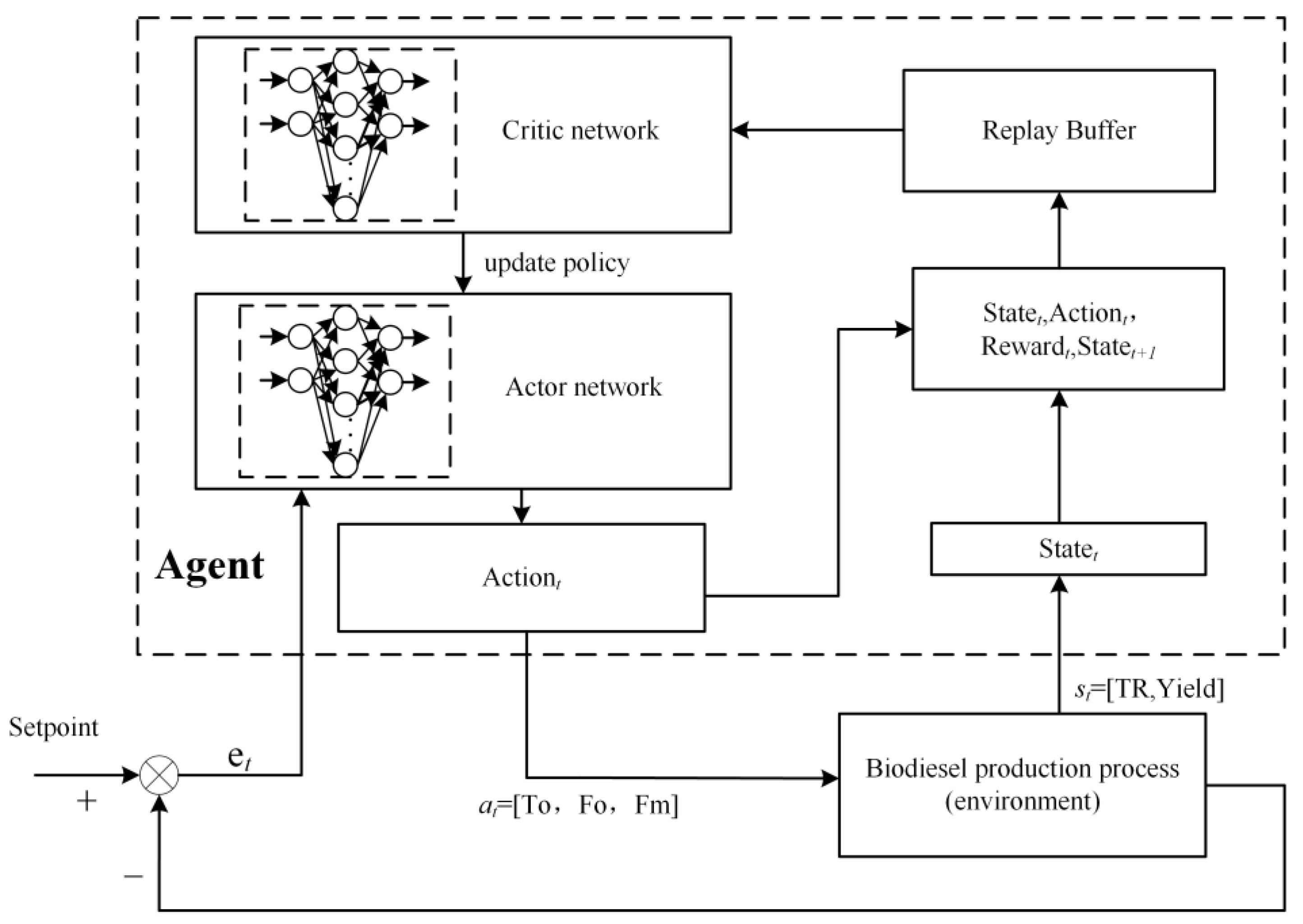
3.3. Control System Framework

In a control system, an agent serves as the controller, while the environment encompasses external factors like industrial processes and sensor data. The objective is to develop an optimal control policy [22,23]. As depicted in Figure 3, the agent interacts with a biodiesel production environment. In deep reinforcement learning, both the state space and action space are pivotal. Unlike traditional supervised learning, the action space in biodiesel production is continuous. The state space is crucial, comprising all potential environmental states.

Table 1. State space information.

State Space
Parameter	Unit	Value Range
$T_R$	Reactor temperature/°C	[40, 62]
$y\text{'}$	Yield/%	[0, 100]

outlines the state space for this specific deep reinforcement learning environment. The input to the state space is a two-dimensional vector $State=\left[T_R,y\text{'}\right]$, where $T_R$ denotes the reactor temperature and $y\text{'}$ signifies the final yield.

In deep reinforcement learning environments, action spaces are typically categorized into discrete and continuous domains [24]. Given the nature of biodiesel production processes, the action space for this specific problem is continuous. The specific actions are represented by $Action=[To,Fo,Fm]$, where $To,Fo,Fm$ correspond to inlet oil temperature, inlet oil flow rate, and inlet alcohol flow rate, respectively. The specific value ranges for these actions are detailed

Table 2. Action space information.

Action Space
Action Parameters	Unit	Value Range
To	Oil temperature/°C	[40, 70]
Fo	Oil flow rate/kg/h	[0, 8000]
Fm	Methanol flow rate/kg/h	[0, 2000]

.

3.4. Reward Function

In deep reinforcement learning algorithms, designing a reward function that aligns with the actual production process is crucial for guiding the agent to learn quickly and efficiently to achieve control objectives. In biodiesel production, process variables are monitored in real time to obtain dynamic data, which are then fed into the TD3 algorithm. The algorithm evaluates the outcome of the current action using a reward function and generates an optimized control output to adjust parameters such as temperature and flow rate, thereby controlling the production process. The reward function is designed based on the deviation between the current state and the desired value, ensuring that the production process always converges to the setpoint.

The reward function is designed based on the error between the current state and the desired value to regulate the entire production process. To achieve this, the function is divided into three components: a primary reward and two auxiliary rewards. The primary reward is calculated as the error between the value $T_R$ and the actual process variable $y\text{'}$. Specifically, the error is computed as $e=|r_{setpoint}-r_{state}|$, set $S=\{e_{TR},e_{\mathrm{yLend}}\}$. An auxiliary reward is provided when both errors are less than a certain threshold. The corresponding reward function is expressed as Equation (14).

$$\begin{array}{c}r=\left\{\begin{array}{ll}\mu e+R\hfill & S_1\le 0.1,S_2\le 0.01\hfill \\ P\hfill & S>e_{\max }\hfill \end{array}\right.\hfill \\ R={\displaystyle \sum _{i=1}^2{\lambda }_i{S}_i}\end{array}$$

(14)

In the equation, $\mu ,\lambda$ is the reward scaling factor that guides the agent’s learning direction. $e$ represents the error between the current state value and the desired setpoint. $e_{\max }$ is the error threshold for the current state value. $R$ is a relatively large reward given when both errors are smaller than their respective thresholds, otherwise, only the smaller reward value will be accepted. When the maximum error threshold $e_{\max }$ is exceeded, the agent will receive a larger penalty.

4. Simulation Experiments and Results

4.1. Experimental Setup

The raw material used in this experiment is palm oil. As the transesterification reaction is highly sensitive to reactor temperature, the primary control objectives are to maintain the reaction temperature and optimize biodiesel yield to ensure complete conversion. The recovered biodiesel product is expected to meet product specifications after methanol recovery.

In this simulation model, feed oil temperature $To$, feed oil flow rate $Fo$, and methanol flow rate $Fm$ are the manipulated variables ($u={[To,Fm,Fo]}^T$). The heat exchanger $Qw$ and methanol temperature $Tm$ are considered as disturbance variables ($d={[Qw,Tm]}^T$). The controlled variables are reactor temperature and yield. The control system is designed to track the setpoints of these variables under fluctuating disturbances $d$, while ensuring that the variables remain within the specified ranges of $u_{\min }={[30,0,0]}^T$, $u_{\max }={[62,8\times {10}^4,2000]}^T$. The disturbance variables are defined within the range of $d_{\min }={[0,30]}^T$, $d_{\max }={[4\times {10}^4,65]}^T$.

Simulations will be conducted to verify the control performance of the TD3 algorithm. The results will be compared with those obtained using traditional PID and NMPC controllers, as well as the DDPG algorithm. For a fair comparison, the hyperparameters of DDPG and TD3 are kept identical, with some key parameters listed in

Table 3. TD3 algorithm parameter settings.

Hyperparameters	Value
Number of rounds	500
Maximum number of steps per training round	1000
Discount factor	0.99
Soft update parameters	5 × 10−3
Actor learning rate	5 × 10−3
Critic learning rate	1 × 10−3
Batch size	64
Noise attenuation rate	1 × 10−5

.

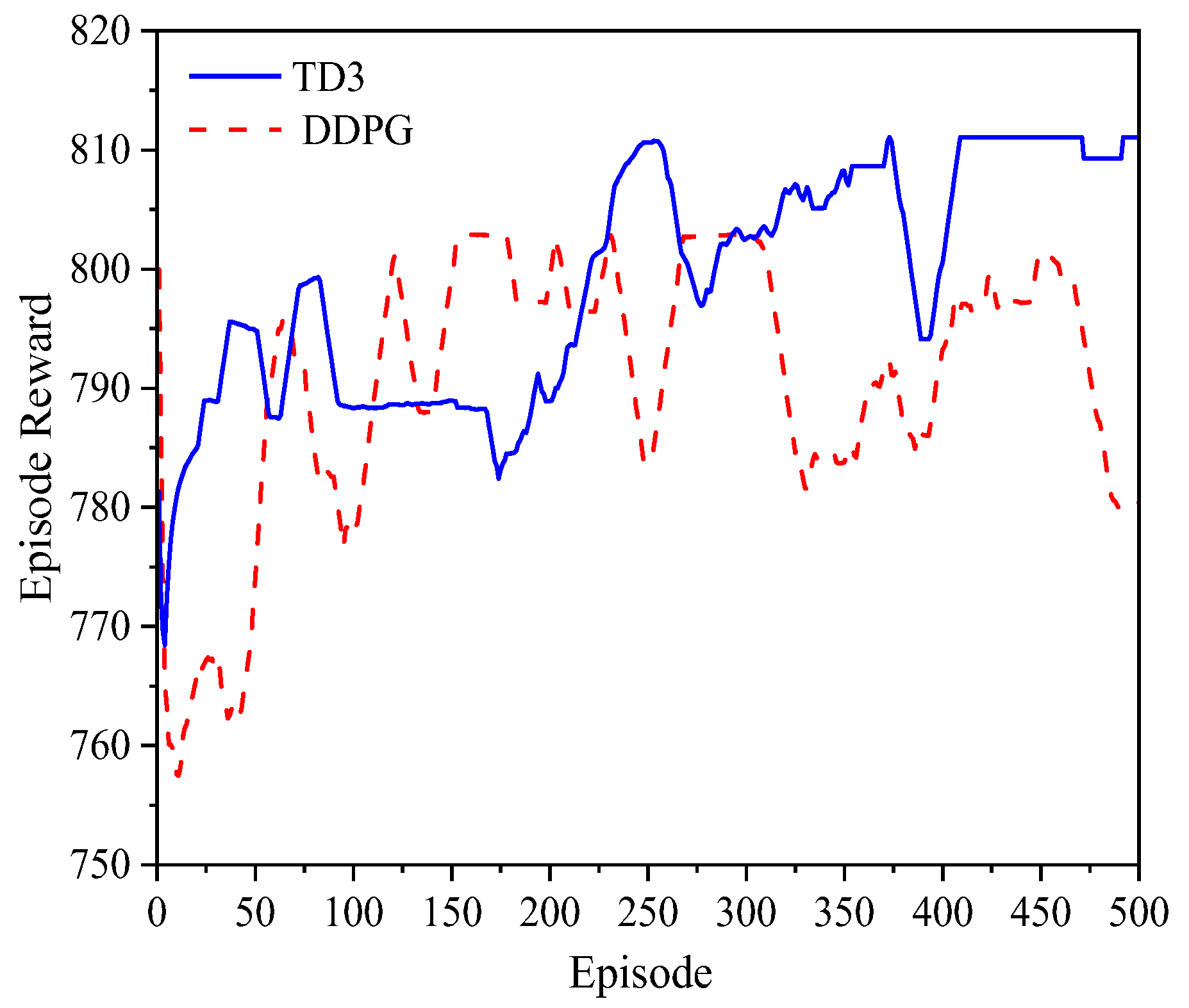
The reward trends for each episode during the training of DDPG and TD3 are shown in Figure 4. By observing the changes in the reward curves of different deep reinforcement learning algorithms during the agent’s training process, it can be found that TD3 converges the fastest. DDPG reaches the optimal solution 150–200 episodes faster than TD3 and can converge within 150 episodes, indicating a faster training speed compared to TD3. This is because the critic network in TD3 uses a value-based learning method, and during the iterative training of the agent, the approximation error will accumulate continuously, leading to value function underestimation, which in turn causes slow training and the risk of falling into local optima. Using two critic networks to estimate the value of an action simultaneously and taking the average of the outputs of each critic network can improve the accuracy of the action value estimation, mitigating the slow training and conservative policy caused by the accumulation of underestimation.

4.2. Simulation Experiment of Expectation Tracking

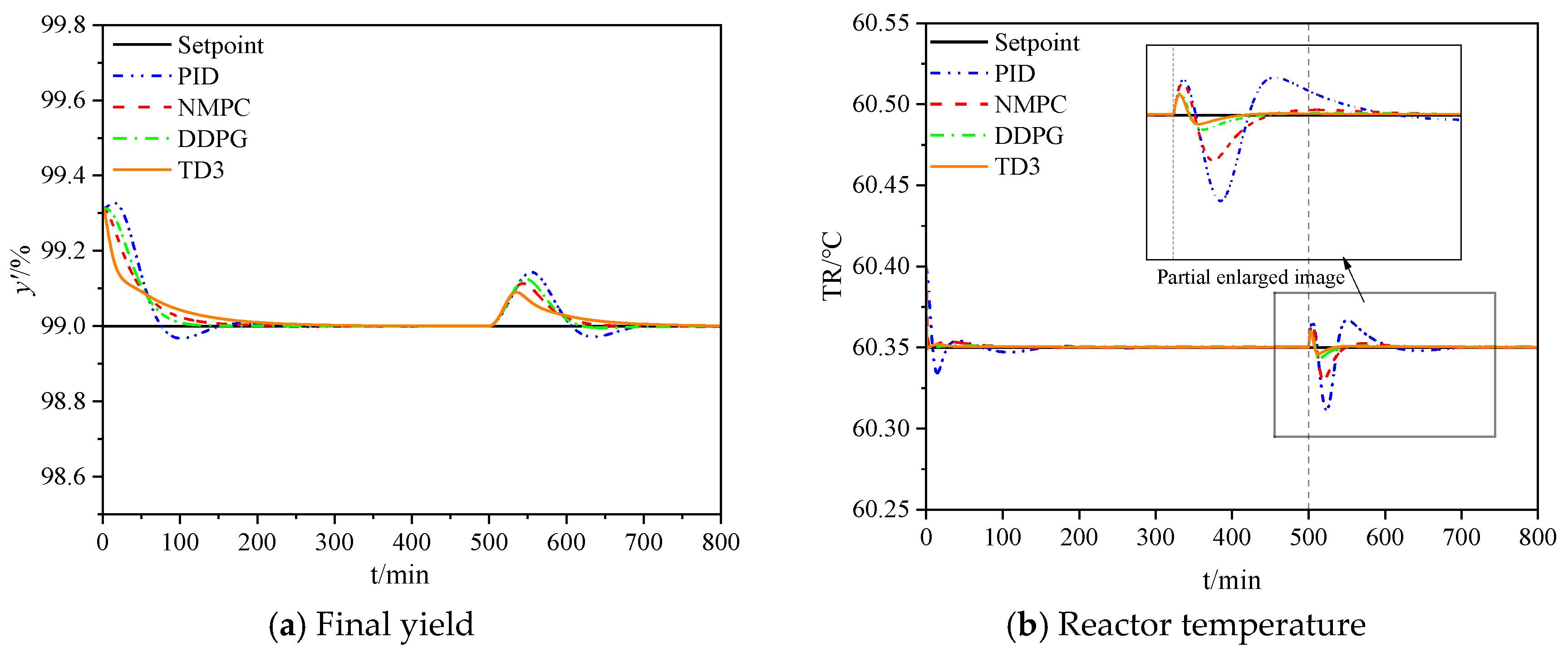
The first set of experiments was designed to evaluate the robustness and dynamic adjustment capability of the control algorithms in a biodiesel production process. The experimental results are shown in Figure 5.

The results indicate that due to initial process instability, both the yield $y\text{'}$ (see Figure 5a) and reactor temperature $T_R$ (see Figure 5b) exhibited small fluctuations around the setpoint. However, as the control algorithms took effect, the system gradually stabilized until the yield converged to the setpoint. At 160 minutes, the yield setpoint was changed to 97% (m/m), causing the system to deviate from the steady state. The TD3 algorithm effectively adjusted the control actions based on the new system state, bringing the yield and reactor temperature back to the desired values.

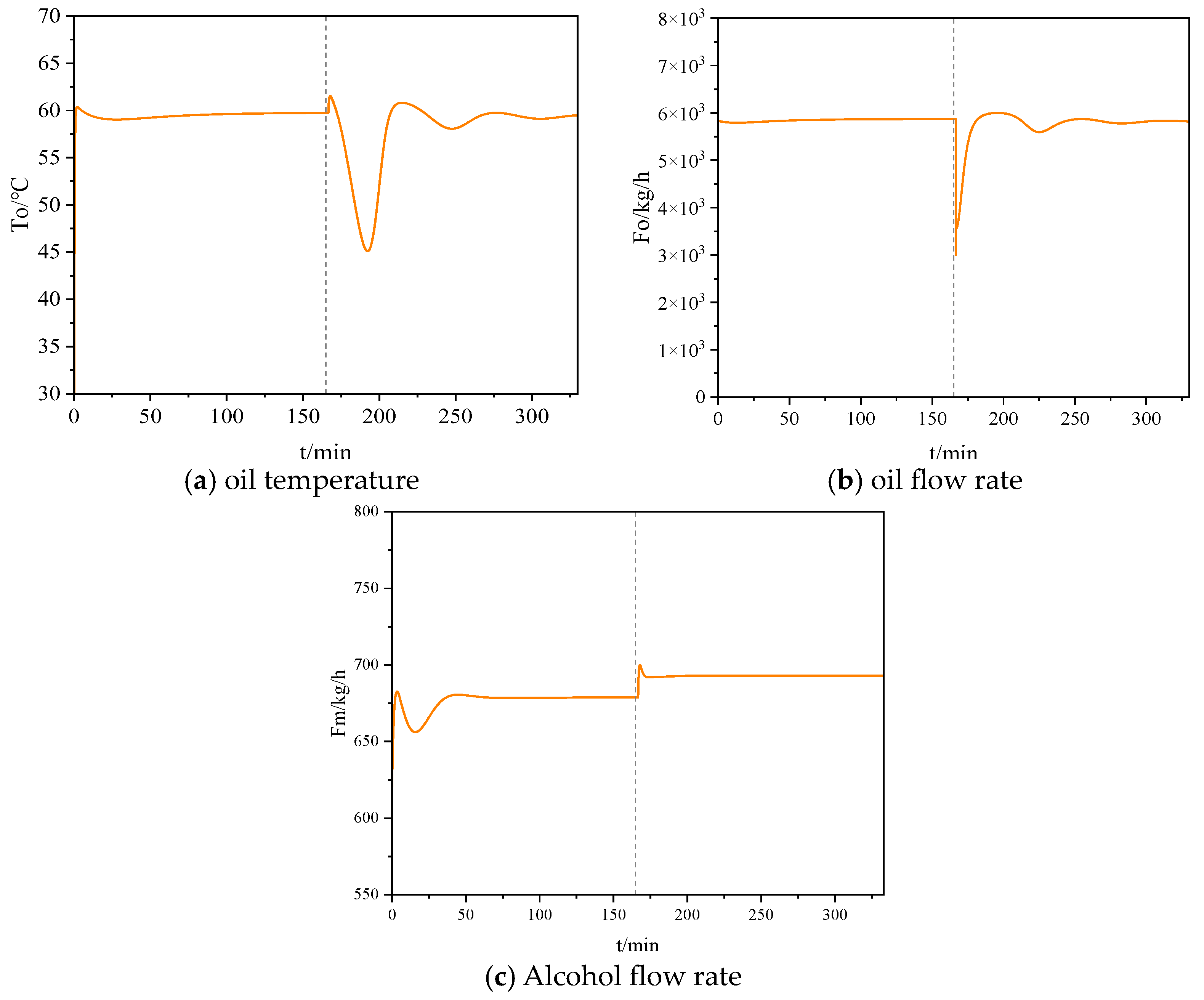
Figure 6 illustrates the variations in inlet oil temperature, alcohol flow rate, and oil flow rate under the TD3 control. To achieve the new yield setpoint, the algorithm reduced the oil flow rate and increased the alcohol flow rate, thereby adjusting the alcohol-to-oil ratio. Moreover, to maintain a suitable reaction temperature, the system controlled the inlet oil temperature to compensate for the temperature fluctuations caused by the introduction of large amounts of cold feedstock.

Comparing the control performance of different algorithms, it is evident that TD3 outperforms both DDPG and traditional control methods in terms of settling time and overshoot. The superior stability of TD3 can be attributed to its rapid convergence capability, which is achieved by employing a dual Q-network and delayed updates, enabling the control system to adapt quickly to environmental changes.

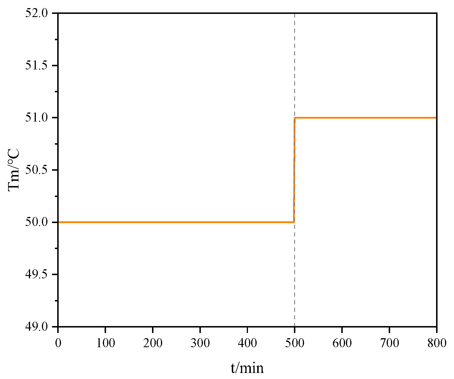
4.3. Simulation Experiment Under Step-Type Noise Input

This section experimentally verifies the ability of the production system to reach a stable state rapidly while simultaneously satisfying the imposed upper and lower constraints under significant external disturbances. In the experiment, the alcohol temperature $Tm$ in the disturbance variable $d={[Qw,Tm]}^T$ was kept constant, and a step change was introduced at a specific time. The noise input variation is shown in Figure 7. Different control algorithms adjusted their inputs based on the changed system state caused by the disturbance, compensating for the noise and returning the reactor temperature to the setpoint.

Under step change conditions, the regulation of final yield $y\text{'}$ and reactor temperature $T_R$ by TD3 and other control algorithms is shown in Figure 8. As shown in Figure 8a,b, TD3 exhibits the fastest recovery and the smallest fluctuations after disturbances, outperforming other algorithms. The control system, under the corrective action of the controller, gradually converges to a steady state.

Table 4. Performance analysis of the different control algorithms.

	Figure 8a			Figure 8b
Comparison Indicators	MSE	MAE	IAE	MSE	MAE	IAE
PID	0.501	170.092	24.119	55.605	1431.203	286.411
NMPC	0.140	145.599	10.135	36.270	1133.423	224.662
DDPG	0.049	98.988	7.290	42.325	1242.396	230.647
TD3	0.029	91.730	5.713	26.001	898.724	223.762

presents the control performance indices of $T_R$ and final yield $y\text{'}$ from Figure 8a,b. Compared with PID, NMPC, and DDPG, TD3 shows significant advantages in control accuracy and stability. The overall system stability is reflected by MSE and IAE, while control robustness is indicated by MAE. Smaller values of MSE, IAE, and MAE represent better performance. The specific calculation methods for MSE, IAE, and MAE are detailed in Appendix B.

Among all the evaluated metrics (MSE, MAE, IAE), the TD3 algorithm consistently demonstrated the best performance in both reactor temperature control and yield control. These results indicate that TD3 offers superior control performance when faced with disturbances, effectively reducing errors and enhancing system stability in both temperature and yield control. This highlights the potential of TD3 as a highly efficient control strategy for complex industrial processes such as biodiesel production.

5. Discussion

This study proposes a novel adaptive optimization control method based on the twin delayed deep deterministic policy gradient (TD3) algorithm to address the challenges of multivariable coupling, nonlinearity, and time delay in biodiesel production. By constructing a simplified biodiesel production model and designing a TD3 controller, simulation experiments demonstrated that the TD3-based control strategy can respond quickly, effectively suppressing fluctuations in temperature and yield and ensuring the stable operation of the production system. Compared to other reinforcement learning algorithms and traditional control methods, TD3 exhibits superior stability and a faster response. The introduction of twin critic networks and delayed updates in TD3 significantly enhances the stability and responsiveness of the control policy, showcasing its potential for complex industrial processes. By leveraging experience replay to learn from past interactions, TD3 can adapt to changing environments and explore new control strategies while exploiting existing ones.

While BDsim serves as a convenient benchmark model due to its simplified assumptions, its applicability may be compromised when dealing with highly variable feedstocks such as waste oil. Although TD3’s twin critic network improves convergence, it relies heavily on computational resources and ample interaction data for effective policy learning. To address these limitations, BDsim’s application can be enhanced by incorporating more real-world experimental data and data-driven models. The substantial computational requirements of TD3 can be mitigated by pre-training and transferring the model to target applications.

When applied to real-world production processes, TD3-based control algorithms can dynamically adjust process parameters in real time, enabling more precise control over raw material and catalyst usage, ensuring product quality stability and reducing production costs. In practical chemical reaction processes, a single control strategy is often insufficient. Combining traditional control methods (such as PID control) with reinforcement learning to form a hybrid control strategy can enhance TD3’s performance under con-strained conditions; this hybrid control strategy can be applied to other complex industrial control processes.