Article

Research on Reactivity-Equivalent Physical Transformation Method for Double Heterogeneity in Pressurized Water Reactors Based on Machine Learning

1
College of Nuclear Science and Technology, Naval University of Engineering, Wuhan 430033, China
2
College of Electrical Engineering, Naval University of Engineering, Wuhan 430033, China
3
Shanghai Institute of Applied Physics, Chinese Academy of Sciences, Shanghai 201800, China
*
Author to whom correspondence should be addressed.
Processes 2024, 12(11), 2493; https://doi.org/10.3390/pr12112493
Submission received: 17 October 2024 / Revised: 4 November 2024 / Accepted: 7 November 2024 / Published: 9 November 2024
(This article belongs to the Section AI-Enabled Process Engineering)

Abstract

:
Traditional computational methods for pressurized water reactors are unable to handle dispersed fuel particles as the double heterogeneity and the direct volumetric homogenization can result in significant errors. In contrast, reactivity-equivalent physical transformation techniques offer high precision for addressing the double heterogeneity introduced by dispersed fuel particles. This approach converts the double heterogeneity problem into a single heterogeneity problem, which is then subsequently investigated by using the conventional pressurized water reactor computational procedure. However, it is currently empirical and takes a lot of time to obtain the right k. In this paper, we train the RPT model by using the existing dataset of plate-dispersed fuel and rod-dispersed fuel by a machine learning method based on a linear regression model, and we then use the new data to make predictions and derive the corresponding similarity ratios. The burnup verification, density verification, fission rate verification, and neutron energy spectrum analysis are calculated through the OpenMC program. For plate-type fuel elements, the method maintains an accuracy within 200 pcm during depletion, with deviations in the 235U density and 235U fission rate within 0.1% and neutron energy spectrum errors within 6%. For rod-type fuel elements, the method maintains an accuracy within 100 pcm during depletion, with deviations in 235U and 239Pu density within 1.5% and neutron energy spectrum errors within 1%. The numerical validation indicates that the reactivity-equivalent physical transformation method based on the linear regression model not only greatly improves the computational efficiency, but also ensures a very high accuracy to deal with double heterogeneity in nuclear reactors.

1. Introduction

Nuclear energy is a clean energy source, which has profound significance in reducing carbon emissions and ensuring energy supplies. In the process of nuclear energy development, nuclear safety is most critical, and the emergence of dispersed particles greatly improves nuclear safety. Dispersed fuels [1] can withstand higher temperatures under some extreme accident conditions and provide excellent intrinsic safety. It is gradually gaining attention in applications due to its excellent characteristics mentioned above. However, the addition of dispersed particles leads to the traditional single heterogeneity becoming a double heterogeneity. Due to the presence of double heterogeneity, traditional neutronics calculation programs are unable to characterize the particle-based dispersion system. To solve the problem of double heterogeneity, reactor physics researchers have proposed numerous approaches. Among many methods, the RPT (reactivity-equivalent physical transformation) method has gradually become a popular topic of research due to its simplicity and efficiency.
In 2005, the concept of the RPT [2] method was introduced to tackle the complexity of fuels with dispersed particles. The strategy entails condensing the dispersed particles into a smaller area while preserving the system’s reactivity at the beginning of the burnup depth, followed by the application of the VWH (volume homogenization method) to the particles located in the condensed region. Thus, the double heterogeneity system is converted to a single heterogeneity system. This method involves no alterations to the existing program’s computational algorithms. Instead, it enhances the accuracy of the results by simply adjusting the geometrical configurations. Furthermore, a novel resonance approach [3] has been introduced to tackle dual heterogeneity. It has been successfully incorporated into the ALPHA program’s resonance module, designed to address the dual heterogeneity challenges, and has shown that the results are of high accuracy. An improved reactivity-equivalent physical transformation (IRPT) method [4] has been put forward to precisely handle FCM fuel with burnable poison particles. This IRPT method is designed to be effective for both criticality and burnup evaluations, and it remains stable regardless of changes in operational parameters. Yet, the conventional RPT approach encounters challenges when attempting to depict systems featuring two types of particles containing poisons. To achieve a uniform distribution of TRISO fuel in high-temperature reactors, the RPT method is applied. For these calculations, the WIMS [5] and Serpent [6] have been employed to address the calculations of the homogenized and double heterogeneous models of TRISO fuel. To manage excessive reactivity and even out the power distribution across the radius, an innovative concept has been put into practice. This involves the application of varying thicknesses of IFBA coating onto the exterior surface of the TRISO particle fuel kernel [7]. Subsequently, neutronic assessments have been carried out, encompassing both two-dimensional full core [8] and three-dimensional full core [9] configurations, where the IFBA coating is uniformly dispersed. Furthermore, the ring reactivity-equivalent physical transformation method (RRPT) has been introduced [10,11], which more accurately simulates the stratified impact of burnable poisons compared to the traditional RPT method. In 2023, the reactive equivalent physical transformation method based on particle diameter (DRPT) [12] was introduced. This DRPT method has demonstrated high precision in dealing with plate heterogenous systems. It is characterized by its straightforward implementation, enhanced outcomes, and broad applicability. The impact of simulating different fuel shapes for the material testing reactor (MTR) is evaluated by building two OpenMC codes [13]. Upon examining the calculations from the two OpenMC models, it was noted that there is a minimal variation in the radial flux distribution, attributable to the similarity in fuel mass. The rapid fitting RPT methods based on the rod fuel elements [14] and the plate fuel elements [15] are proposed. The results show that the model with high fitting accuracy has practical engineering application value.
As the technology continues to evolve, machine learning is now expanding into the field of reactor analysis as a key tool for building alternative models for complex large-scale numerical computational programs. In 2022, Suubi Racheal [16] proposed a novel approach to train machine learning model and use augmented datasets reflecting sensor states. This study develops, trains, and compares three machine learning models: support vector machines (SVMs), decision trees (DTs), and multilayer perceptrons (MLPs). The results show that SVM and DT models perform better than MLP models. In 2023, Zhenhai Liu [17] carried out research on machine learning-based methods for constructing equivalent models for fuel rod temperature distribution. This study aimed to improve the computational efficiency of large-scale fuel rod performance simulation, and the construction strategy of the equivalent model for predicting the temperature distribution of fuel rods was discussed and analyzed in detail using fuel rod temperature prediction as a research example. The results show that the constructed equivalent model has a computational speedup of about 204 times compared to the COPERNIC program with high accuracy. In 2023, Guanghu [18] elaborated five DDML algorithms such as linear regression (LR), principal component analysis (PCA), and artificial neural network (ANN), and DDML showed good applicability in the simulation of multi-scale and multi-physics fields. Artificial intelligence and machine learning (AI/ML) technologies offer unique opportunities to transform nuclear plant operations and power generation. In 2024, the barriers to AI/ML adoption within the nuclear power industry were discussed [19], with a focus on existing commercial reactors. In 2024, HaoWu [20] developed an automated tree-based machine learning method for the nuclear pebble bed of the high temperature gas-cooled reactor (HTGR) to explore the complex thermal radiation behavior. The findings indicate that the AutoML model operates approximately 5 to 10 times more swiftly compared to conventional techniques. Additionally, the Pareto front of the AutoML model reveals that the mean square error diminishes as the model complexity is reduced, culminating in the attainment of the optimal solution. At present, the application of machine learning and artificial intelligence in the field of nuclear engineering is in a developing state, and there is still room for improvement. For example, in calculating the kinf of a reactor, deterministic calculations for the core under a two-step framework have a computation cost at the level of around ten minutes, which provides sufficiently accurate results. Using machine learning for prediction can be faster, but it requires a large amount of simulated data for training initially, and the trained system cannot be used for different reactor types.
Through research and analysis, it has been found that the RPT method has been widely studied due to its simple and efficient advantages. However, most of them adopt traditional methods to obtain the similarity ratio of the RPT model, which requires the calculation of a large number of Monte Carlo program results and consumes a significant amount of time. Therefore, this paper connects machine learning with the RPT model; machine learning algorithms can automatically establish the RPT model, significantly improving the efficiency of obtaining the similarity ratio of the RPT model. The obtained RPT model can be calculated by using a conventional neutronics program.

2. Materials and Methods

This section provides an introduction to RPT methods and machine learning, and the RPT method based on machine learning is proposed.

2.1. Reactivity-Equivalent Physical Transformation

Figure 1 is a schematic diagram of the traditional RPT method. Initially, all the dispersed particles are compressed within a smaller fuel region; subsequently, for the compressed fuel region, homogenization is performed by using the volume weighting method, and the conventional pressurized water reactor physics calculation procedures are applied. In the RPT method, by ensuring that the kinf of the system is equal to the reference solution, the radius of the compressed fuel region is determined. The reference solution is obtained through high-fidelity deterministic codes or Monte Carlo procedures.
As depicted in Figure 2, a conventional RPT method for plate-shaped structures is introduced, which is an extension of the RPT method designed for cylindrical geometries. The principle behind the plate geometry RPT closely mirrors that of the cylindrical counterpart, with the key distinction being the rectangular fuel region in the plate, influenced by both its length and width dimensions. To address this, the concept of equivalent side lengths is introduced. These lengths represent the dimensions of the fuel area after reduction, where both the length and width are scaled down uniformly. The equivalent edge lengths are also bounded by the upper and lower bounds. The upper bound should not surpass the original fuel area’s dimensions, while the lower bound corresponds to the minimal length and width when all fuel particles are compressed to the fuel zone’s center. Typically, the exact equivalent side lengths fall within these upper and lower bounds.
A straightforward computational illustration of applying the RPT method to fuel plates with dispersed particles is provided in the central part of Figure 2. It is supposed that the fuel region of the plate element has a length of a, a width of b, and a height of H, with a packing fraction f for the dispersed particles.
1. The dispersed particles are compacted within a certain area, with both the length and width being reduced proportionally. Both a and b are scaled down by factor s, resulting in the new dimensions as and bs. The factor s is the similarity ratio (SR) of the fuel plate with its maximum value. Equation (1) is derived from the principle of maintaining the volume consistency of the dispersed particles.
2. The novel composite fuel material is synthesized via volumetric blending within the compacted fuel zone, with the matrix between the original and the newly formed fuel zones remaining unchanged. The nuclear number density is preserved across both the downsized fuel area and the initial fuel area. Consequently, the final RPT model for the fuel plate incorporating dispersed particles is formulated for this particular similarity ratio.
f × a × b × H = a × b × H × s 2
s = f
Range of similarity ratios: ( f ,1).

2.2. Introduction to Machine Learning RPT Method Based on Linear Regression Model

Machine learning based on linear regression modeling is a common supervised learning method used to predict the output of a continuous value. In linear regression, a linear relationship is assumed between the dependent variable (output) and the independent variable (characteristics). The model describes the relationship between the features and outputs by fitting the best possible straight line that minimizes the error between the predicted outputs and the actual observations. The basic form of the linear regression model can be expressed as Equation (2).
y = ω 0 + ω 1 x 1 + ω 2 x 2 + + ω n x n
where y is the predicted value, ω 0 , ω 1 , ω 2 , ....., ω n are the parameters (weights) of the model, and x 1 , x 2 , ..., x n are the input features. The essence of a linear regression model is to use the explanatory variables to estimate the mean of the explanatory variables through the least squares method. Find the best-fit straight line by obtaining the sum of the squares of the residuals between the minimized observations and the model predictions. By extracting the independent variables and creating and fitting a linear regression model, the predictions are made to the model to obtain the predicted values. In order to assess the performance of a model, it can be validated by using various metrics, such as the mean square error or coefficient of determination. These metrics measure the fit of the model to the observed data and its predictive ability, and then finally, the optimal parameters are adjusted to obtain the best prediction value required. In the RPT method, the compressed fuel equivalent radius is determined by ensuring that the kinf of the system is equal to the reference solution. The reference solution is again obtained by a high-fidelity deterministic program or a Monte Carlo program. However, all are currently obtained empirically by spending a lot of time iterating in order to obtain the corresponding k∞. Therefore, this paper is based on the machine learning approach that can quickly derive the similarity ratios of the corresponding dispersed fuel particles. The principle of obtaining the similarity ratio is that the kinf of the equivalent model is equal to the kinf under the direct explicit particle modeling condition. The computational predictions are made by linear regression modeling for the parameters in the plate fuel element and rod fuel element that have a significant effect on the RPT model. The similarity ratios corresponding to them are finally obtained. The modeling process is described below: This model trains and predicts a linear regression model for a given dataset by using the Linear Regression model of the sklearn library.
  • Data loading and preprocessing
First, the training data are loaded from the training set file by using the loadtxt function of the numpy library, and spaces are used as separators. We need to preprocess the data to extract features f, R, and S and target variable SR by a slicing operation.
2.
Linear regression model creation and training
By importing the LinearRegression class in the sklearn.linear_model module and instantiating the LinearRegression object after the data are preprocessed, a linear regression model is created. The fit method of the model pass the feature matrix x and the target variable y as parameters into the model for training in order to observe the model parameters by printing the coefficients coef_ and intercept intercept_ of the model.
3.
Model Prediction and Evaluation
After training the model, the model can be used to predict new data. First, load the test data in the test set file, extract the features f, R, S and the target variable SR, and then call the predicted method of the model to obtain the predicted values. In order to evaluate the performance of the model, the error calculation is also added, in addition to using the matplotlib library to plot the graphs of the true target and predicted values in order to compare the difference between them more intuitively.
4.
Prediction of new data
In addition to making predictions on the test data, we can also use the trained model to make predictions on unseen data. By creating a dataFrame object in pandas containing new feature values and using the model to make predictions, we can quickly apply the model to a new dataset and obtain predictions. In the next section, we will analyze the prediction of new rod and plate element parameters.

3. Results

In this section, the RPT method is investigated based on machine learning for both rod fuel elements and plate fuel elements. For the plate fuel element, three of the RPT parameters will be analyzed and calculated, which are shown in Table 1. For the rod fuel element, six of the RPT parameters will be analyzed and calculated, which are shown in Table 2. The results are validated and analyzed with conventional Monte Carlo calculations.

3.1. Plate-Type Component RPT Calculation Based on Linear Regression Model

Among the three parameters of the selected plate element, the value range of R is 0.015–0.04, the value range of S is 0.72–0.72 × 1.52, and the value range of f is 0.1–0.3. The SR is the actual similarity ratio calculated from these three parameters. The three parameters R, S, and f and the corresponding similarity ratio SR are selected from the existing data, and a total of 19 groups are shown in Table 3, which are used for training the model. The prediction results are shown in Figure 3 and Table 4.
A quantitative and qualitative analysis of the machine learning model’s process will be provided here. Table 3 and Table 5 represent the data used for model prediction for rod-type and plate-type fuel elements, respectively. For plate-type elements, the f, R, and S are the independent variables while SR is the dependent variable. For rod-type elements, Rpf, Rpar, Rcf, ρmod, f, and L are the independent variables, while SR is the dependent variable. After the data are preprocessed, a LinearRegression object is instantiated by using the LinearRegression class in the sklearn.linear_model module. With this, a linear model is trained. Table 4 and Table 6 display the similarity ratios and absolute deviations between the two, thereby analyzing the relevant physical properties through the similarity ratios. This is a flowchart to facilitate the understanding of the paper’s structure which is shown in Figure 4.
Through Figure 3, it can be seen that the linear regression model has a better training effect, and the predicted data curves are basically close to overlap. It shows that the method of machine learning to deal with the plate element RPT is more accurate and can meet the practical needs.

3.2. Calculation of RPT for Rod Elements Based on Linear Regression Modeling

The six parameters and the corresponding similarity ratio SR are selected from the existing data, and a total of 21 groups are shown in Table 5, which are used for training the model. The trained model is used to predict five new datasets in Table 6.
In comparison of the final obtained results, the absolute errors are kept in the thousandths of a percentile, and the relative errors are kept within 1%. It can be seen through Figure 5 that the linear regression model is trained better and that the predicted data curves basically overlap. This indicates that the machine learning approach handles the rod element with high accuracy and meets the practical requirements.

3.3. Numerical Validation and Analysis

3.3.1. Plate Fuel Element Validation Analysis

In this section, the OpenMC [21] program is used to validate the similarity ratios of the predicted RPT parameters of the plate elements above. It includes the k inf , G M calculated by the actual similarity ratio and the k inf , R P T calculated by the predicted similarity ratio. SR_PRED is the predicted similarity ratio. The results of the kinf -deviation are shown in Table 7, and the kinf -deviation is shown in Equation (3).
k d e v i a t i o n = ( k inf R P T k inf G M ) × 10 5
From Table 7, it can be concluded that both kinf deviations are small and that the deviations are kept within 200 pcm, which meets the actual accuracy requirements. Among them, Case5 has the largest deviation of 146 pcm and Case3 has the smallest deviation of 18 pcm.

Burnup Verification

In Section 3.3.1, Case3 and Case5 are selected to validate the GM model and RPT model for burnup, and Figure 6 and Figure 7 demonstrate the variation of kinf during the burnup process.
The overall trend in both remains consistent: the kinf decreases with increasing burnup depth. In Case3, the RPT model curves basically overlap with the GM model curves, the maximum deviation is less than 200 pcm, and they overall were maintained within 100 pcm. The maximum error is 168.62 pcm at a burnup depth of 1.037 MWd/t, and the minimum deviation is 13.384 pcm at a burnup depth of 4.666 MWd/t. In Case5, the RPT model curves basically coincide with the GM model curves and the maximum deviation is 108.85 pcm at a burnup depth of 4.66575 MWd/t. The minimum deviation is 13.357 pcm at a burnup depth of 2.592 MWd/t. This indicates that the RPT model maintains a high accuracy over the full lifetime of the burnup.

235U Density Verification

Case3 with the smallest kinf deviation and Case5 with the largest kinf deviation in Table 7 are selected to validate the 235U density against the GM model and the RPT model, and Figure 8 and Figure 9 demonstrate the variation of 235U density with burnup.
The general trend remains consistent for both, with the 235U density decreasing as the depth of burnup increases. It is obvious in both figures that the GM model curves overlap completely with the RPT model curves, and the relative errors show an increasing trend but are of a small order of magnitude. At a burnup depth of 5.869 MWd/t, the maximum error is 0.00284% which is negligible. This indicates that the 235U density of the RPT model is basically unaffected by the fit over the full lifetime of the burnup and meets the practical accuracy requirements.

235U Fission Rate Validation

Case3 with the smallest kinf deviation and Case5 with the largest kinf deviation in Table 7 are selected to validate the 235U fission rate for the GM model and RPT model, and Figure 10 and Figure 11 demonstrate the variation of the 235U fission rate with burnup.
In the case with the smallest kinf deviation, the maximum error is 0.021% at a burnup depth of 2.592 MWd/t. In the case with the largest kinf deviation, the maximum error is 0.011% when the burnup depth reaches 6.221 MWd/t. This indicates that the 235U fission rate of the RPT model is basically unaffected by the fit over the full life of the burnup and meets the practical accuracy requirements.

Neutron Energy Spectrum Analysis

The neutron energy spectrum delineates the spread of neutrons within the reactor based on their energy levels. Case3 with the smallest kinf deviation and Case5 with the largest kinf deviation in Table 7 are selected to analyze the neutron energy spectrum of the GM model and the RPT model. Figure 12 and Figure 13 demonstrate the variation in neutron fluxes with neutron energies and the relative errors.
In the low-energy region, the relative errors of the GM model and the RPT model are large. For Case3, the relative error is 6.55% at an energy of 1.23 × 10⁻³ eV. For Case5, the relative error is 5.10% at an energy of 1.23 × 10⁻³ eV. The trends of the energy spectra of the GM and RPT models are basically the same in the middle- and high-energy regions. The deviation of the RPT model in the resonance region fluctuates significantly in both cases due to the partial loss of the self-shielding effect, but the deviation is within 2%.

3.3.2. Rod Fuel Element Validation Analysis

In this section, the OpenMC program will be used to validate the similarity ratios of the five sets of data for the rod element, and the results of its kinf deviation are shown in Table 8.
From Table 8, it can be concluded that the deviation between k inf , R P T calculated by the model and the actual value of rod fuel k inf , G M is small, being kept within 100 pcm. It indicates that the linear regression model fits well and meets the requirement of practical accuracy.

Burnup Verification

Case3 with the smallest kinf deviation and Case1 with the largest kinf deviation in Table 8 are selected to validate the GM model and RPT model with burnup, and Figure 14 and Figure 15 show the variation of k inf , G M and k inf , R P T with burnup.
For Case3 and Case1, the general trends remain consistent, both decreasing with an increasing burnup depth. In Case3, the RPT model curve basically coincides with the GM model curve, and the pcm shows a monotonically increasing trend. The maximum deviation is less than 50 pcm. The maximum error is 48.7 pcm at a burnup depth of 19.25 MWd/t, and the minimum error is 45.7 pcm at a burnup depth of 1.75 MWd/t. In Case1, the RPT model curve is basically coincident with the GM model curve, and the pcm shows a monotonically increasing trend, with the maximum deviation not exceeding 100 pcm. The maximum error is 98.7 pcm at a burnup depth of 19.25 MWd/t, and the minimum error is 93.6 pcm at a burnup depth of 1 MWd/t. This indicates that the fitting effect of the RPT model is very stable and can maintain a high accuracy during the burnup lifetime.

235U, 239Pu Density Verification

Case3 with the smallest kinf deviation and Case5 with the largest kinf deviation in Table 8 are selected to validate the 235U and 239Pu densities of the GM model and the RPT model, Figure 16 and Figure 17 illustrate the variation in the 235U density with burnup, and Figure 18 and Figure 19 illustrate the variation in the 239Pu density with burnup.
As can be seen from the figure, the general trend remains the same for both, with the 235U density decreasing during the burnup. In Case3, the maximum error is 0.1965% when the burnup depth reaches 0.25 MWd/t; in Case5, the maximum error is negligible at 0.2216% when the burnup depth is at the initial value.
As can be seen from the figure, the general trend remains the same for both, with the 239Pu density decreasing during the burnup. In Case3, the maximum error is 0.643% when the burnup depth reaches 19.25 MWd/t; in Case5, the maximum error is 0.823% when the burnup depth reaches 19.25 MWd/t, which is negligible. This indicates that the 235U density and 239Pu density of the RPT model are basically unaffected by the fitting during the burnup lifetime and meet the practical accuracy requirements.

Neutron Energy Spectrum Analysis

The distribution of neutrons within a reactor based on their energy is represented by the neutron energy spectrum. Case3 with the smallest kinf deviation and Case1 with the largest kinf deviation in Table 8 are selected to analyze the neutron energy spectrum of the GM model and the RPT model, and the variation in neutron fluxes with neutron energies and the flux relative errors are demonstrated in Figure 20 and Figure 21.
The relative errors between the GM model and the RPT model are smaller in the low-energy and medium-energy regions. The fluctuations in the resonance region of the high-energy region are obvious, but the relative errors are all within 0.445%, which is negligible and meets the actual accuracy requirements.

4. Conclusions

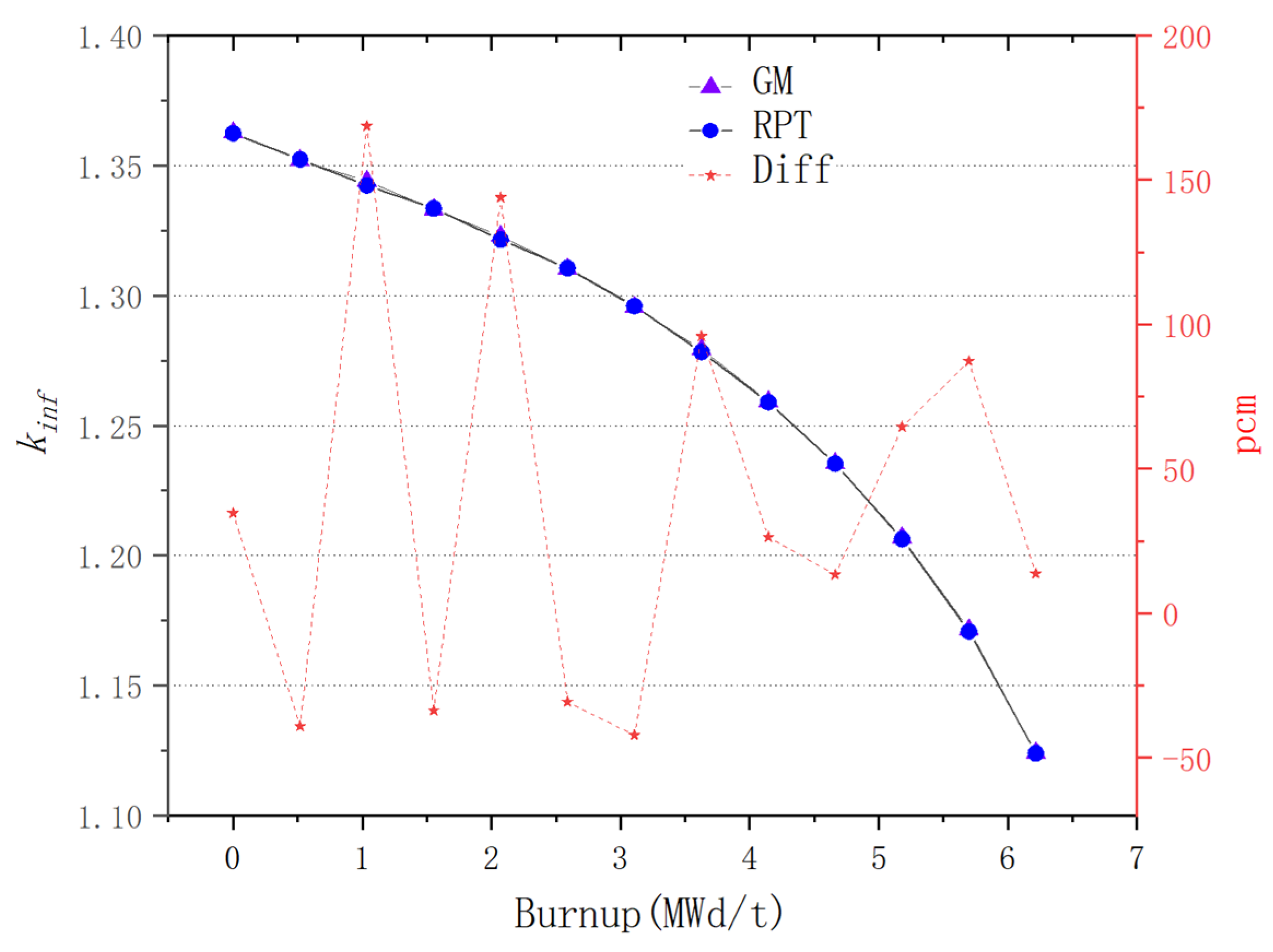
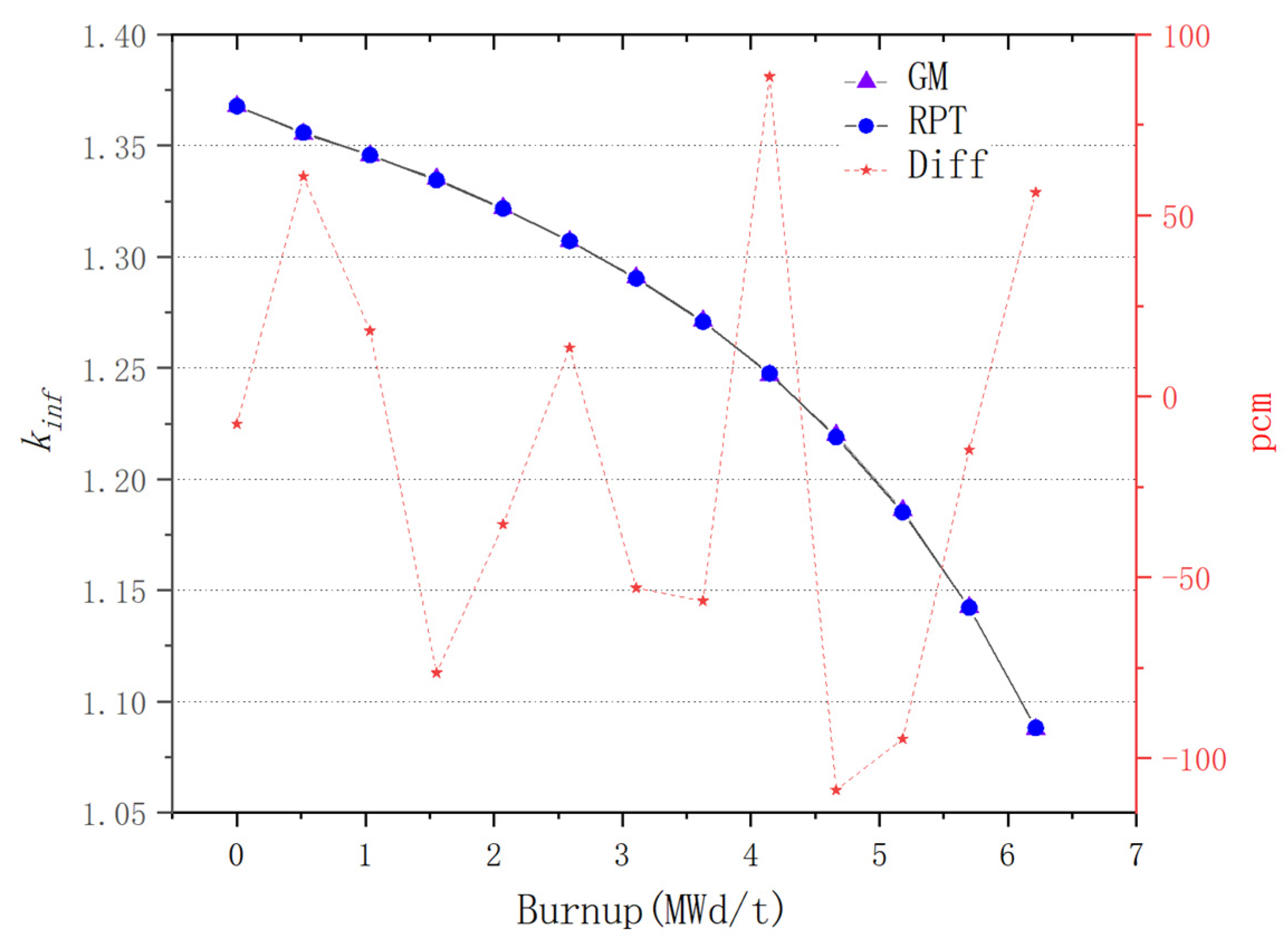
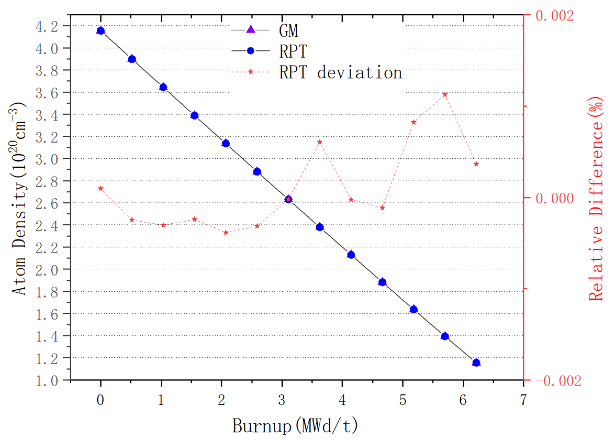
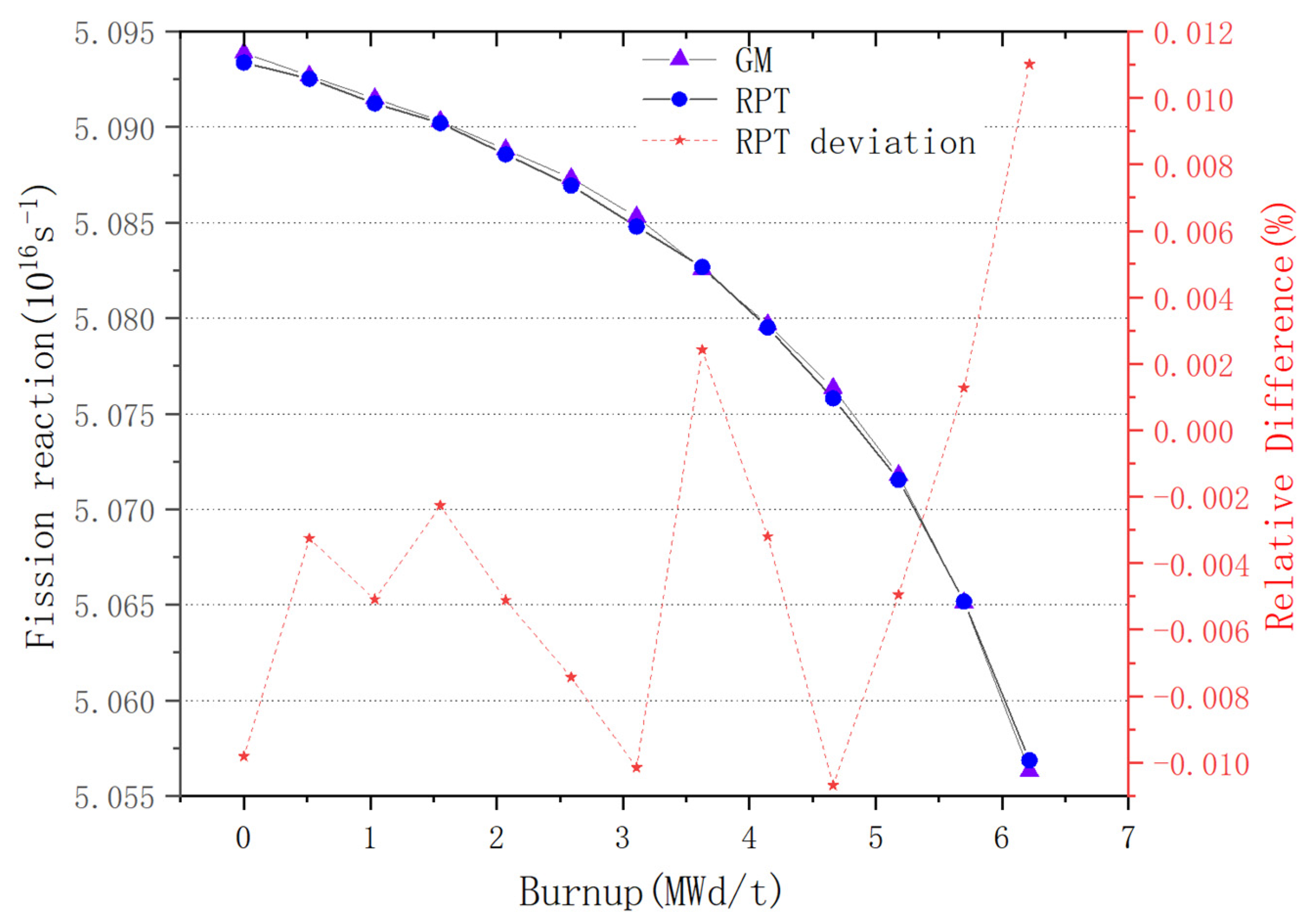
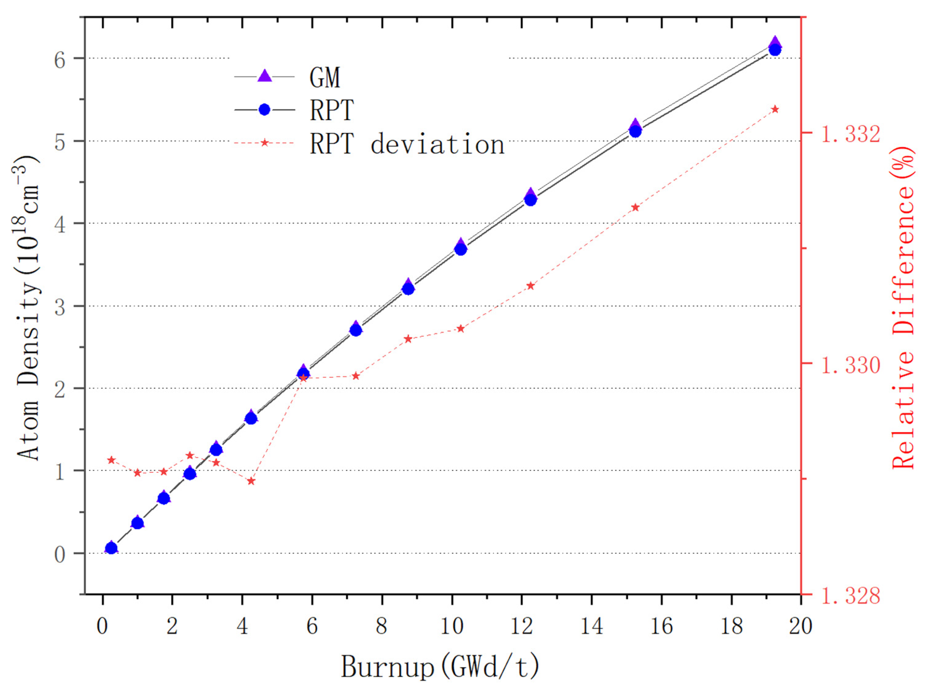
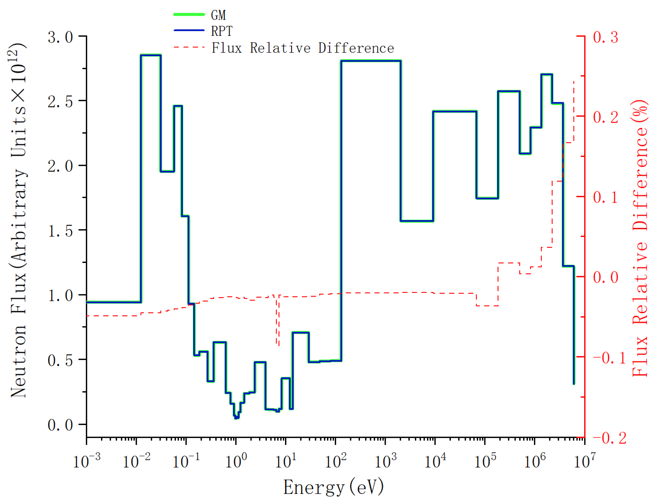
In this paper, the reactive-equivalent physical transformation method, which is based on machine learning, is used to calculate and predict the RPT parameters of plate-dispersed fuel particles and rod-dispersed fuel particles through a linear regression model, and the similarity ratio of the corresponding parameters is derived. The equivalent radius or equivalent side length of the RPT model is calculated using the similarity ratios. The burnup verification, density verification, fission rate verification, and neutron energy spectrum analysis are carried out by OpenMC programs.
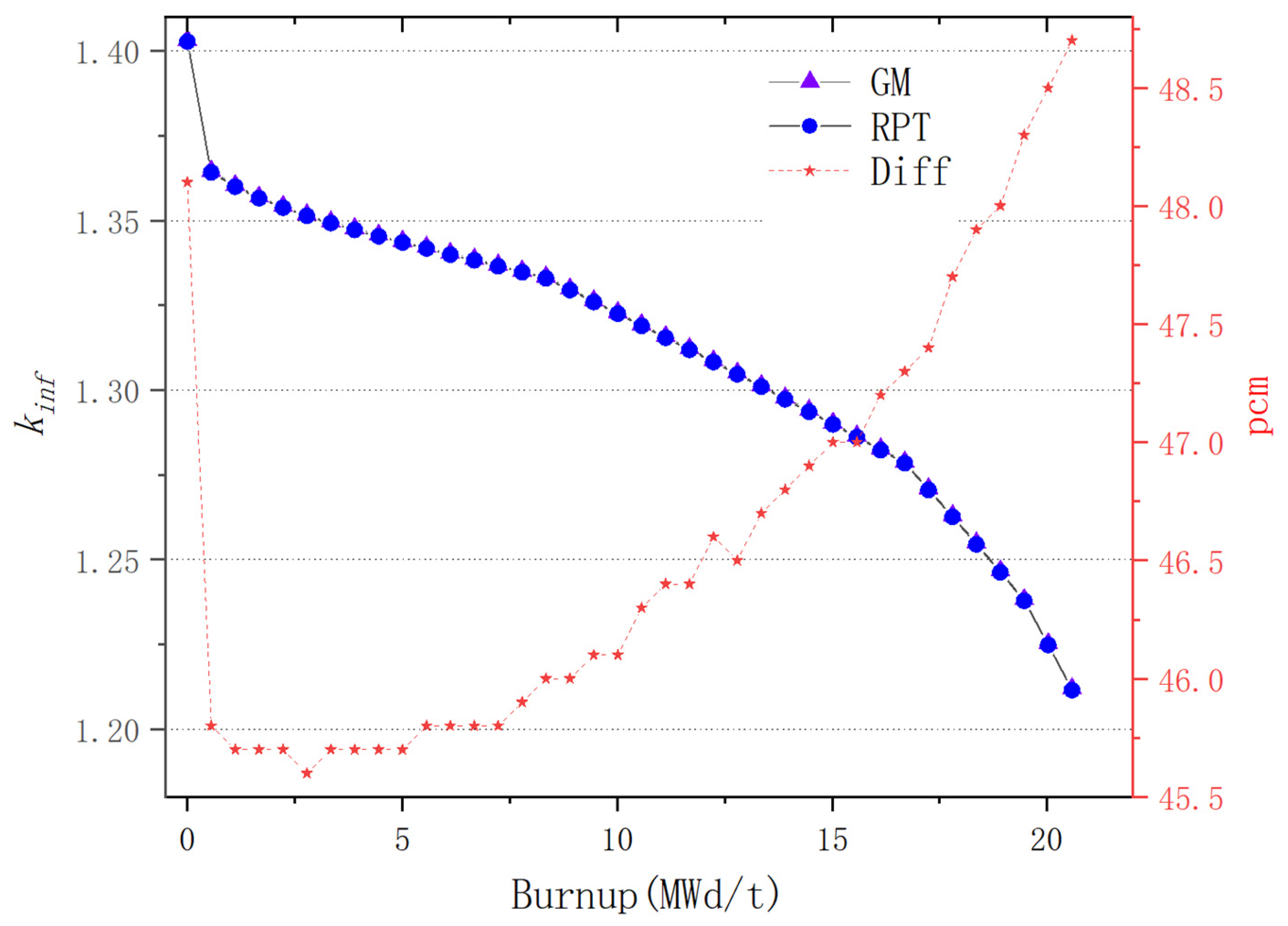
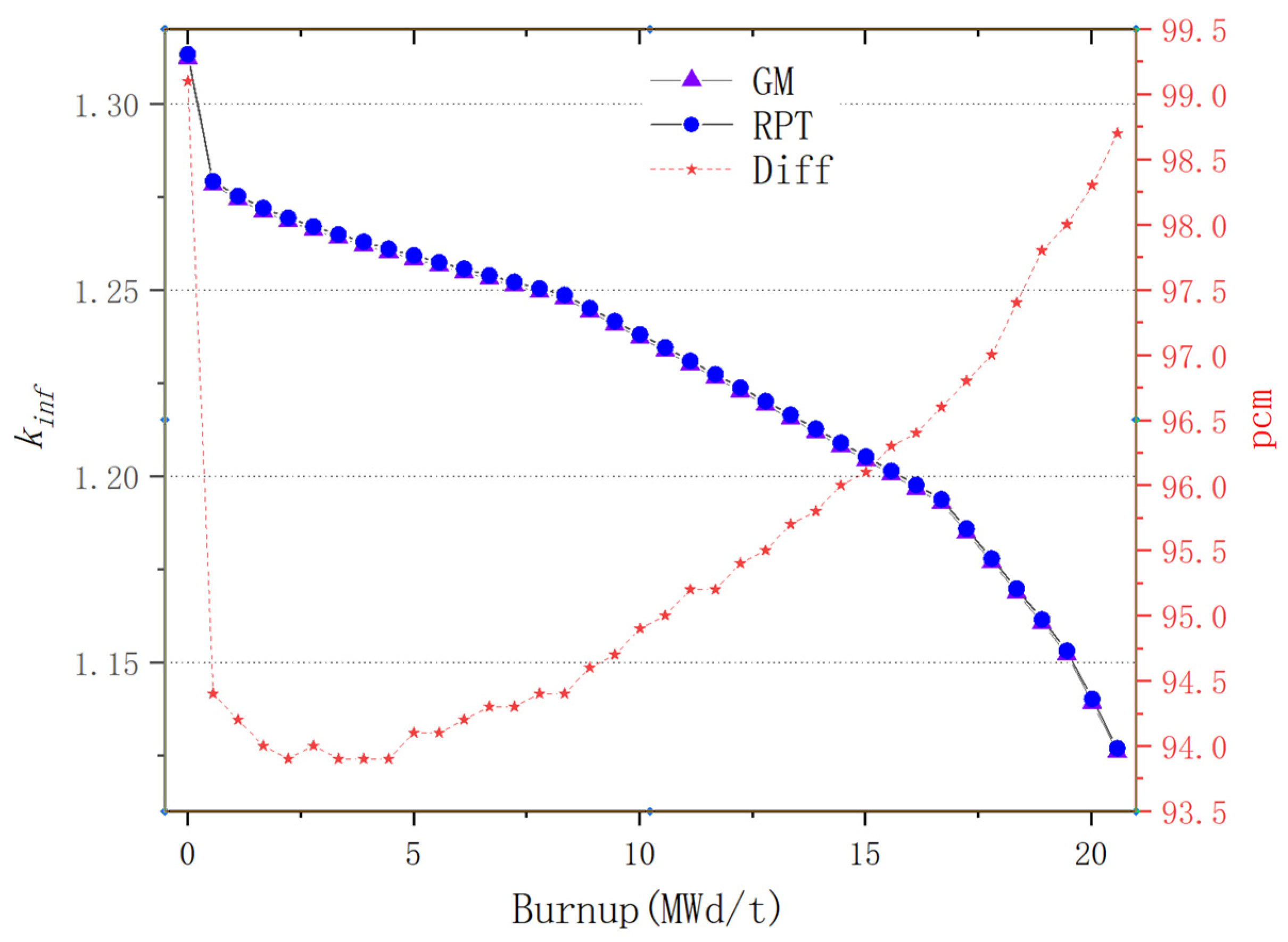
For plate-type fuel elements, among the five cases used for verification, the maximum error is 146 pcm and the minimum error is 18 pcm. These two cases with the maximum and minimum errors are selected for further verification. Both cases maintain a high level of accuracy during depletion, with the maximum errors being 168 pcm and 109 pcm, respectively. It stays within 200 pcm during depletion. Additionally, both cases maintain a high level of accuracy in the 235U density and fission rate, with errors within 0.1%. Regarding the neutron energy spectrum, the maximum errors for both cases occur in the low-energy range, at 6.55% and 5.1%, respectively. High accuracy is maintained in the medium- and high-energy ranges, with errors within 2%. For rod-type fuel elements, among the five cases used for verification, the maximum error is 99 pcm and the minimum error is 48 pcm. These two cases with the maximum and minimum errors are selected for further verification. Both cases maintain a high level of accuracy during depletion, with the maximum errors being 99 pcm and 49 pcm, respectively. It stays within 100 pcm during depletion. For the 235U and 239Pu density, the maximum error in both cases is within 1.5%. Regarding the neutron energy spectrum, unlike the plate-type fuel elements, high accuracy is maintained in the low-energy range, and while the error increases in the high-energy range, it remains within 1%. The data results show that the reactivity-equivalent physics transformation method based on the linear regression model not only has greatly improved the computational efficiency, but also ensures a very high accuracy, which meets the needs of practical usage.

Author Contributions

J.L. and S.L. proposed the research point, conducted the program coding and manuscript writing. L.L. and B.H. participated in the machine learning process. L.C. and Y.Z. (Yongfa Zhang) supervised this study. J.H. and Y.Z. (Yunfei Zhang) participated in the work of the RPT formula derivation. All authors have read and agreed to the published version of the manuscript.

Funding

This work is supported by the following sources the National Natural Science Foundation of China (No. 12305198), China Postdoctoral Science Foundation (No. 2022M48884), and the Natural Science Foundation of Hubei province (No. 2023AFB341).

Data Availability Statement

The original contributions presented in the study are included in the article, further inquiries can be directed to the corresponding author.

Conflicts of Interest

The authors declare that they have no known competing financial interests or personal relationships that could have appeared to influence the work reported in this paper.

References

  1. Dam, H.V. Long-term control of excess reactivity by burnable particles. Ann. Nucl. Energy 2000, 27, 733–743. [Google Scholar] [CrossRef]
  2. Kim, Y.; Kim, K.; Noh, J. Reactivity-Equivalent Physical Transformation for Homogenization of Double-Heterogeneous Fuels. In Proceedings of the Transactions of Korean Nuclear Society Autumn Meeting, Busan, Republic of Korea, 27–28 October 2005. [Google Scholar]
  3. Li, S.; Zhang, Q.; Zhang, Z.; Zhao, Q.; Liang, L.; Liang, Y.; Zhang, J.; Lou, L. Evaluation of improved subgroup resonance treatment based on Sanchez-Pomraning method for double heterogeneity in PWR. Ann. Nucl. Energy 2020, 143, 107491. [Google Scholar] [CrossRef]
  4. Li, J.; She, D.; Shi, L. An improved reactivity equivalent physical transformation for treating FCM fuel with burnable poisons. Ann. Nucl. Energy 2018, 121, 577–581. [Google Scholar] [CrossRef]
  5. Alrwashdeh, M.; Alameri, S.A.; Alkaabi, A.K.; Ali, M. Homogenization of TRISO Fuel using Reactivity Equivalent Physical Transformation Method. Transactions 2019, 121, 1521–1522. [Google Scholar]
  6. Leppanen, J.; Pusa, M.; Viitanen, T.; Valtavirta, V.; Kaltiaisenaho, T. The Serpent Monte Carlo code: Status, development and applications in 2013. Ann. Nucl. Energy 2015, 82, 142–150. [Google Scholar] [CrossRef]
  7. Alrwashdeh, M.; Alameri, S.A.; Alkaabi, A.K. Preliminary Study of a Prismatic- Core Advanced High-Temperature Reactor Fuel Using Homogenization Double- Heterogeneous Method. Nucl. Sci. Eng. 2020, 194, 163–167. [Google Scholar]
  8. Alrwashdeh, M.; Alameri, S.A. Two-Dimensional Full Core Analysis of IFBACoated TRISO Fuel Particles in Very High Temperature Reactors. In International Conference on Nuclear Engineering; American Society of Mechanical Engineers: New York, NY, USA, 2020; Volume 83761, p. V001T05A014. [Google Scholar]
  9. Alameri, S.A.; Alrwashdeh, M. Mohammad. Preliminary three-dimensional neutronic analysis of IFBA coated TRISO fuel particles in prismatic-core advanced high temperature reactor. Ann. Nucl. Energy 2021, 163, 108551. [Google Scholar] [CrossRef]
  10. Lou, L.; Yao, D.; Chai, X.; Peng, X.; Li, M.; Li, W.; Yu, Y.; Wang, L. A novel reactivity-equivalent physical transformation method for homogenization of double-heterogeneous systems. Ann. Nucl. Energy 2020, 142, 107396. [Google Scholar] [CrossRef]
  11. Lou, L.; Chai, X.; Yao, D.; Peng, X.; Chen, L.; Li, M.; Yu, Y.; Wang, L. Research of ring RPT method on spherical and cylindrical Double-Heterogeneous systems. Ann. Nucl. Energy 2020, 147, 107741. [Google Scholar] [CrossRef]
  12. Li, P.; Hao, C.; Zhou, X.; Zhang, Z. Research on the method for dealing with plate fuel systems with double heterogeneity. Harbin Gongcheng Daxue Xuebao/J. Harbin Eng. Univ. 2023, 44, 1597–1604. [Google Scholar]
  13. Alaa, H.A.; Ahmed, A.A.; Abdullah, I.A. Investigation of the Fuel Shape Impact on the MTR Reactor Parameters Using the OpenMC Code. Processes 2023, 11, 637. [Google Scholar] [CrossRef]
  14. Zhang, Y.; Zhang, Q.; Zhang, J.; Wang, X.; Lou, L.; Liu, G.; Zhao, Q.; Zhang, Z. A comprehensive evaluation of the RPT method on FCM fuel in light water reactor. Ann. Nucl. Energy 2020, 142, 107434. [Google Scholar] [CrossRef]
  15. Li, J.; Chen, L.; Li, S.; Zhang, Y.; Hao, J.; Zhang, Y.; Chen, G. Evaluation of the fitting-based reactivity-equivalent physical transformation method for double heterogeneity phenomena of plate-type fuel in pressurized water reactors. Ann. Nucl. Energy 2024, 207, 110677. [Google Scholar] [CrossRef]
  16. Racheal, S.; Liu, Y.; Ayodeji, A. Evaluation of optimized machine learning models for nuclear reactor accident prediction. Prog. Nucl. Energy 2022, 149, 104263. [Google Scholar] [CrossRef]
  17. Liu, Z.; Qi, F.; Zhou, Y.; Li, H.; Li, W.; Zeng, W.; Xin, Y.; Wang, H.; Ma, C. Based on machine learning fuel rod temperature distribution agent model construction method research. Nucl. Power Eng. 2023, 44, 1–5. [Google Scholar]
  18. Hu, G.; Pfingsten, W. Data-driven machine learning for disposal of high-level nuclear iste: A review. Ann. Nucl. Energy 2023, 180, 109452. [Google Scholar] [CrossRef]
  19. Hall, A.; Agarwal, V. Rodriers to adopting artificial intelligence and machine learning technologies in nuclear power. Prog. Nucl. Energy 2024, 175, 105295. [Google Scholar] [CrossRef]
  20. Wu, H.; Hao, S.; Niu, F.; Tu, J. A tree-based automated machine learning approach of the obstructed view factor of thermal radiation in nuclear pebble beds. Prog. Nucl. Energy 2024, 173, 105261. [Google Scholar] [CrossRef]
  21. Romano, P.K.; Forget, B. The OpenMC Monte Carlo particle transport code. Ann. Nucl. Energy 2013, 51, 274–281. [Google Scholar] [CrossRef]
Figure 1. Basic principles of the RPT method for rod elements.
Processes 12 02493 g001
Figure 2. Basic principles of the plate-type component RPT method.
Processes 12 02493 g002
Figure 3. Similarity ratio of the plate RPT model.
Processes 12 02493 g003
Figure 4. Flowchart of applying machine learning models.
Processes 12 02493 g004
Figure 5. Similarity ratio of the rod RPT model.
Processes 12 02493 g005
Figure 6. Variation with burnup for minimum kinf deviation.
Processes 12 02493 g006
Figure 7. Variation with burnup at maximum kinf deviation.
Processes 12 02493 g007
Figure 8. Variation of 235U density with burnup at the minimum kinf deviation.
Processes 12 02493 g008
Figure 9. Variation of 235U density with burnup at the maximum kinf deviation.
Processes 12 02493 g009
Figure 10. Variation of 235U fission rate with burnup at the minimum kinf deviation.
Processes 12 02493 g010
Figure 11. Variation of 235U fission rate with burnup at maximum kinf deviation.
Processes 12 02493 g011
Figure 12. Variation in neutron flux with neutron energy at minimum kinf deviation.
Processes 12 02493 g012
Figure 13. Variation in neutron flux with neutron energy at maximum kinf deviation.
Processes 12 02493 g013
Figure 14. Variation with burnup for minimum kinf deviation.
Processes 12 02493 g014
Figure 15. Variation with burnup at maximum kinf deviation.
Processes 12 02493 g015
Figure 16. Variation of 235U density with burnup at the minimum kinf deviation.
Processes 12 02493 g016
Figure 17. Variation of 235U density with burnup at the maximum kinf deviation.
Processes 12 02493 g017
Figure 18. Variation of 239Pu density with burnup at the minimum kinf deviation.
Processes 12 02493 g018
Figure 19. Variation of 239Pu density with burnup at maximum kinf deviation.
Processes 12 02493 g019
Figure 20. Variation in neutron flux with energy at the minimum of kinf deviation.
Processes 12 02493 g020
Figure 21. Variation in neutron flux with energy at maximum kinf deviation.
Processes 12 02493 g021
Table 1. Plate-type element parameters.
NoParametersComment
1ROuter radius of the fuel kernel
2fPacking fraction
3SFuel area size
Table 2. Rod-type element parameters.
NoParametersComment
1RpfOuter radius of the fuel kernel
2RparOuter radius of the particle
3RcfOuter radius of the cell fuel zone
4LLength of the cell
5ρmodDensity of moderator
6fPacking fraction
Table 3. Plate element RPT training parameters.
CasefR (cm)S (cm2)SR
10.150.020.87120.896
20.250.031.03680.925
30.30.0351.620.943
40.20.040.720.845
50.250.021.21680.952
60.150.0251.620.89
70.20.031.41120.915
80.10.0151.03680.89
90.150.031.41120.87
100.20.0351.03680.875
110.250.0351.21680.91
120.150.0250.87120.868
130.250.020.87120.953
140.10.0151.620.905
150.250.041.03680.895
160.250.0251.03680.94
170.20.021.620.952
180.30.0351.03680.92
190.150.0251.21680.89
Table 4. Plate element RPT training parameters.
CaseSRSR_PREDAbsolute Error
10.9070270.913651550.00662455
20.8706810.880277450.00959645
30.925950.932971480.00701248
40.851750.860957520.00920752
50.8968750.891396890.00547811
Table 5. Rod element RPT parameters (training).
CaseRpfRparRcffLρmodSR
10.0320.0530.60.361.5970.530.791587
20.0380.0520.590.411.6890.850.88578
30.0290.0550.60.391.6020.940.771288
40.0340.050.60.471.6830.670.879322
50.0290.0560.560.381.6690.90.758034
60.0360.0530.610.511.6610.960.872503
70.030.0490.590.431.720.60.867403
80.030.0550.550.341.680.610.750047
90.0270.0490.560.471.7580.980.871202
100.0380.0510.590.521.6050.610.886234
110.0360.0490.560.411.7280.780.922807
120.0290.0530.580.51.7450.640.841566
130.0320.0520.610.511.7530.910.882943
140.0340.0490.60.371.720.670.887217
150.0320.0490.580.531.6230.520.870648
160.030.0550.570.431.6220.980.777879
170.0370.050.560.421.6170.70.886357
180.0340.0490.560.461.7130.70.908090
190.0280.050.560.391.6080.530.794398
200.0320.050.550.361.6340.740.828195
210.0320.0490.550.341.7620.520.866093
Table 6. Rod element RPT training parameters.
CaseSR_GMSR_PREDAbsolute Error
10.7639090.769321570.00541257
20.8362350.832308780.00392622
30.8493290.852835240.00350624
40.8782680.884980190.00671219
50.8999110.907178440.00726744
Table 7. Deviation in verification of plate fuel elements.
Case k i n f , G M k i n f , R P T SR_PREDkinf-Deviation (pcm)
11.334931.335160.91365223
21.391461.392630.880277117
31.362641.362820.93297118
41.369381.370480.860958110
51.366391.367510.891397146
Table 8. Actual and predicted kinf and deviation of kinf for rod fuel.
Case k i n f , G M k i n f , R P T SR_PREDkinf-Deviation (pcm)
11.3122221.3132130.7693215799.1
21.3605581.3599700.8323087858.8
31.4027001.4031810.8528352448.1
41.4528121.4536290.8849801981.7
51.4709161.4717340.9071784481.8
Disclaimer/Publisher’s Note: The statements, opinions and data contained in all publications are solely those of the individual author(s) and contributor(s) and not of MDPI and/or the editor(s). MDPI and/or the editor(s) disclaim responsibility for any injury to people or property resulting from any ideas, methods, instructions or products referred to in the content.

