A Leakage Safety Discrimination Model and Method for Saline Aquifer CCS Based on Pressure Dynamics

Abstract

The saline aquifer CCS is a crucial site for carbon storage. Safety monitoring is a key technology for saline aquifer CCS. Current CO₂ leakage detection methods include microseismic, electromagnetic, and well-logging techniques. However, these methods face challenges, such as difficulties in determining CO₂ migration fronts and predicting potential leakage events; as a result, the formulation of test timing and methods for these safety monitoring techniques are somewhat arbitrary. This study establishes a gas–water two-phase seepage model and solves it using a semi-analytical method to obtain the injection pressure and the derivative curve characteristics of the injection well. The pressure derivative curve can reflect the physical properties of the reservoir through which CO₂ flows underground, and it can also be used to determine whether CO₂ leakage has occurred, as well as the timing and amount of leakage, based on boundary responses. This study conducted sensitivity analyses on eight parameters to determine the impact of each parameter on the bottom-hole pressure and its derivatives, thereby obtaining the influence of its parameters on different flow stages. The research indicates that, when a steady-state flow characteristic appears at the outer boundary, CO₂ leakage will occur. Additionally, the leakage location can be determined by calculating the distance from the injection well. This can guide the placement and measurement of safety monitoring methods for saline aquifer CCS. The method proposed in this paper can effectively monitor the timing, location, and amount of leakage, providing a technical safeguard for promoting CCS technology.

1. Introduction

With the rapid economic development of modern society, China’s demand for energy has significantly increased, indirectly leading to higher emissions of greenhouse gases such as CO₂, which has caused severe environmental problems, as even small temperature changes can significantly disrupt the balance of the Earth’s ecosystem. For example, rising sea levels pose great threats to low-lying coastal areas, global climate change is severe, and freshwater resources are scarce [1]. Carbon capture and storage (CCS) is the most promising technology for industrial-scale emission reductions [2]. Currently, numerous CCS projects are in operation and under construction worldwide. According to a report by the Global CCS Institute (GCCSI), as of August 2018, there are 38 large-scale CCS projects, either in operation or under construction, globally. Of these, the 18 operational CCS projects collectively capture only about 32 million tonnes of CO₂ annually [3].

Compared to the rest of the world, China’s CCS technology started relatively late. The Shenhua CO₂ Saline Aquifer Storage Project is the first full-chain CCS project in China. Storage safety is a critical indicator of the project’s success. To demonstrate storage safety, the project employs various monitoring methods, including vertical seismic profile (VSP) monitoring [4]. China began its investment in CCS technology with a series of government policies. From 2006 to 2008, the government issued several documents, including the National Medium- and Long-Term Science and Technology Development Plan (2006–2020), the National Climate Change Program, the National Special Action on Climate Change Science and Technology, and China’s Policies and Actions for Addressing Climate Change, progressively designating CO₂ capture, utilization, and storage technology as key national research and development projects [5]. Subsequently, major national projects, such as the 973 Program’s “Resource Utilization and Underground Storage of Greenhouse Gases for Enhanced Oil Recovery” and the 863 Program’s “CO₂ Capture and Storage Technology”, began to conduct further in-depth research on CCS technology [6]. CO₂ geological storage has been piloted in several countries and has stepped into the industrial preparation phase [7]. However, two core issues remain unresolved: injectivity and safety. Regarding storage safety assessments, the National CO₂ Geological Storage Capacity Assessment Demonstration Project was launched by the China Geological Survey in 2010 [8]. Through the joint efforts of over 20 organizations, China has established an early-stage technical methods and indicator system for CO₂ geological storage [9].

The issue of storage safety is the premise and foundation for the success of CO₂ saline aquifer storage projects. Without resolving or clearly understanding safety, a project’s feasibility cannot be ensured [10]. So-called storage safety refers to the process of ensuring that, within the designed injection rate and total injection volume, the injected CO₂ does not cause destructive damage to the formation or result in earthquakes or leakage [11]. There are many factors that affect the safety of storage; primarily, the characteristics of the formation. During the site selection phase, therefore, it is essential to gather as much detailed data as possible on storage site characteristics, including geological data of reservoir–cap assemblages [12]. Based on the collected geological data, an injection plan should be formulated, specifying the injection control temperature and pressure. Moreover, early monitoring and warning are crucial safety barriers. For example, monitoring points can be designed above the primary cap rock to monitor its integrity [13]. If a leak in the primary cap rock is detected, immediate confirmation and timely remedial measures can be taken to prevent the stored CO₂ from spreading to other areas [14].

This study proposes a cutting-edge theoretical judgment method based on on-site testing results and suggests using pressure dynamics to determine CO₂ leakage. Based on pressure dynamics, for the first time, this paper establishes a saline aquifer CCS leakage safety discrimination model, which is solved through a semi-analytical method to obtain the injection pressure and the derivative curve characteristics of the injection well. The pressure derivative curve can reflect the physical properties of CO₂ flowing underground through the reservoir and determine whether CO₂ leakage occurs based on the boundary response. At present, most on-site CO₂ leakage detection methods rely on atmospheric monitoring, logging monitoring, etc., which require a large amount of work and are high-cost. This study predicts the leakage of CO₂, which is economically efficient and can provide timely warnings.

2. Mathematical Model

Safety monitoring is a crucial technology for saline aquifer CCS. This section focuses on establishing a physical model and a mathematical model for the leakage safety discrimination model for saline aquifer CCS based on pressure dynamics from the perspective of seepage mechanics. Additionally, a dimensionless mathematical model is established.

2.1. Physical Model

Predicting CCS leakage in saline aquifers is a difficult problem in current research with limited relevant data. This paper proposes a cutting-edge method for predicting CCS leakage in saline aquifers based on pressure dynamics, which has not been applied in practice. This article aims to conduct safety monitoring of CCS in saline water layers, ignoring the dissolution of CO₂ in saline aquifer layers.

During the initial stage of multicomponent gas injecting, the displacement efficiency near the injection well is low, making it difficult to establish a pure gas region. Typically, a gas-rich water–gas region (also called a transitional region) is formed near the well. At the same time, the distant area remains unswept by saline water (referred to as the saline water region). Therefore, based on fluid distribution, properties, and pressure changes during the initial stage of gas flooding, a radial composite well testing model for the two regions near the injection well can be established, as shown in Figure 1. The assumptions of the physical model during the initial stage of multicomponent gas flooding are as follows:

(1)

The effects of the wellbore reservoir and the skin effects of the injection well are considered;

(2)

During the initial gas flooding period, the inner region is considered the transition region. Based on research results on the distribution characteristics of fluid thermodynamic properties, it can be concluded that the fluid mobility and storage coefficient in the transition region exhibit an exponential relationship with radial distance, as shown in Figure 1 and Equations (1) and (2);

(3)

According to research findings on the pressure distribution characteristics between different regions, it has been shown that, due to the additional resistance at the interface between the transition region and the saline water region, the pressure exhibits a discontinuous decline. This section uses the interfacial skin factor to describe the additional pressure drop characteristics at the interface between the transition region and the saline water region, as shown in Figure 2;

(4)

The fluids in different regions of the formation are assumed to be slightly compressible fluids, neglecting the influence of gravity and capillary forces;

(5)

The formation can be categorized as an infinite, closed, or constant pressure type;

(6)

During gas flooding, the fluid flow characteristics are assumed to take on an isothermal Darcy flow;

(7)

Reservoir characteristics are assumed to be horizontally homogeneous and isotropic;

(8)

The initial pressure of the reservoir remains constant and equal everywhere.

(9)

Although the model relies on simplified assumptions, such as neglecting gravity and capillary forces, that may lead to inaccuracies, particularly in heterogeneous reservoirs, these simplifications help streamline the computational process. This model is an analytical model, which is solved using semi-analytical methods to prepare for the actual model.

$${\left(k/\mu \right)}_1={\left(k/\mu \right)}_{*}\cdot {\left({\displaystyle \frac{r}{r_w}}\right)}^{-\theta }$$

(1)

$${\left(\phi c_t\right)}_1={\left(\phi c_t\right)}_{*}\cdot {\left({\displaystyle \frac{r}{r_w}}\right)}^{-I}$$

(2)

In the equation:

${(k/\mu )}_1$—Fluid mobility in the transition region during the initial stage of gas flooding, $\mathrm{mD}\cdot {\mathrm{cp}}^{-1}$;

${(k/\mu )}_{*}$—Fluid mobility at the bottom of the well during the initial stage of gas flooding, $\mathrm{mD}\cdot {\mathrm{cp}}^{-1}$;

$\theta$—Power-law index of fluid mobility variation in the transition region during the initial stage of gas flooding, which is dimensionless;

${\left(\phi c_t\right)}_1$—Fluid storage coefficient in the transition region during the initial stage of gas flooding, ${\mathrm{MPa}}^{-1}$;

${\left(\phi c_t\right)}_{*}$—Fluid storage coefficient at the bottom of the well during the initial stage of gas flooding, ${\mathrm{MPa}}^{-1}$;

$I$—Power-law index of the fluid storage coefficient’s variation in the transition region during the initial stage of gas flooding, which is dimensionless;

$r$—Distance from the reservoir to the injection well, m;

$r_w$—Wellbore radius, m;

This model is a 2D model. Due to the limited number of on-site sealing examples, the model proposed in this study is a theoretical exploration in preparation for practical models.

2.2. Mathematical Model Establishment

Seepage Differential Equation

The seepage model was constructed in the form of polar coordinates and with reference to the well test analysis method.

The seepage model of the transition region can be deduced as follows:

$${\displaystyle \frac{1}{r}}{\displaystyle \frac{\partial }{\partial r}}\left({\left({\displaystyle \frac{k}{\mu }}\right)}_{1}r{\displaystyle \frac{\partial p_1}{\partial r}}\right)={\displaystyle \frac{{\left(\varphi c_t\right)}_1}{3.6}}{\displaystyle \frac{\partial p_1}{\partial t}},r_w\le r<R_m$$

(3)

In the same way, the seepage model of the saline water region can be described as follows:

$${\displaystyle \frac{1}{r}}{\displaystyle \frac{\partial }{\partial r}}\left({\left({\displaystyle \frac{k}{\mu }}\right)}_{2}r{\displaystyle \frac{\partial p_2}{\partial r}}\right)={\displaystyle \frac{{\left(\varphi c_t\right)}_2}{3.6}}{\displaystyle \frac{\partial p_2}{\partial t}},R_m\le r<R_e$$

(4)

The inner boundary condition is a constant flow boundary which is shown below.

$$\underset{r\to r_w}{lim}(r{\displaystyle \frac{\partial p_1}{\partial r}})={\displaystyle \frac{1.842\times 10^{-3}{\mu }_{*}{B}_{*}q}{kh}}$$

(5)

In the equations:

${\mu }_1^{*}$— Fluid viscosity at the bottom of the well, $\mathrm{cp}$;

$B_1^{*}$—Volume coefficient of the fluid at the bottom of the well;

Outer Boundary Condition:

There are three types of outer boundary conditions, namely infinite reservoir, circular constant pressure boundary, and circular closed boundary.

Infinite reservoir:

$$p_2(r\to \infty ,t)=p_i$$

(6)

Circular constant pressure boundary:

$$p_2(r=R_e,t)=p_i$$

(7)

Circular closed boundary:

$${\displaystyle \frac{\partial p_2(r=R_e,t)}{\partial r}}=0$$

(8)

The continuity condition at the interface between the transition region and the saline water region follows the principle of equal flow rates, and the interfacial skin factor is used to describe the additional pressure drop characteristics at the interface:

$$\left\{\begin{array}{c}{p}_1(r=R_m,t)=p_2(r=R_m,t)-{\left(S_{1}r{\displaystyle \frac{\partial \left(p_2\right)}{\partial r}}\right)}_{r=R_m}\\ {\left({\displaystyle \frac{k}{\mu }}\right)}_1{\displaystyle \frac{\partial \left(p_1\right)}{\partial r}}(r=R_m,t)={\left({\displaystyle \frac{k}{\mu }}\right)}_2{\displaystyle \frac{\partial \left(p_2\right)}{\partial r}}(r=R_m,t)\end{array}\right.$$

(9)

The pressure is equal throughout the reservoir at the initial time:

$$p_1(r,t=0)=p_2(r,t=0)=p_i$$

(10)

The dimensionless process is described in Appendix A.

3. Mathematical Model Solution

We used mathematical methods to solve the leakage safety discrimination model established in the previous section and to describe the detailed solution process. We now transform the above dimensionless mathematical model and boundary conditions using the Laplace equation for transformation:

$${\overline{P}}_D={\int }_0^{\infty }{e}^{-s{t}_D}{P}_D(r_D,t_D)d{t}_D$$

(11)

Consequently, we obtain the general solution of the Bessel function in terms of the dimensionless radius for the inner and outer regions:

$${\overline{P}}_{1D}=A_1{r}_D^{\gamma }{I}_v\left(\xi r_D^{\beta }\right)+A_2{r}_D^{\gamma }{K}_v\left(\xi r_D^{\beta }\right)$$

(12)

$${\overline{P}}_{2D}=A_3{I}_0\left(r_D\sqrt{s}\right)+A_4{K}_0\left(r_D\sqrt{s}\right)$$

(13)

In the equation:

$$\gamma ={\displaystyle \frac{\theta }{2}}\begin{array}{cc} \beta ={\displaystyle \frac{\theta -I+2}{2}}& \upsilon ={\displaystyle \frac{\theta }{\theta -I+2}}\end{array} \xi ={\displaystyle \frac{\sqrt{s}}{\beta }}$$

(14)

Equation (28) is the general solution of the Bessel function for the inner and outer regions of the dimensionless radius. Substituting Equation (12) into the inner boundary condition Equation (20), we obtain:

$$a_{11}{A}_1+a_{12}{A}_2+a_{13}{A}_3+a_{14}{A}_4=1$$

(15)

In the equation:

$$a_{11}=-s\sqrt{s}{I}_{v-1}\left(\sqrt{s}\right)$$

(16)

$$a_{12}=s\sqrt{s}{K}_{v-1}\left(\sqrt{s}\right)$$

(17)

$$a_{13}=0$$

(18)

$$a_{14}=0$$

(19)

Substituting Equations (12) and (13) into the interface continuity condition of Equation (A14), we obtain:

$$a_{21}{A}_1+a_{22}{A}_2+a_{23}{A}_3+a_{24}{A}_4=0$$

(20)

In the equation:

$$a_{21}=R_{mD}^{\gamma }{I}_v\left(\xi R_{mD}^{\beta }\right)$$

(21)

$$a_{22}=R_{mD}^{\gamma }{K}_v\left(\xi R_{mD}^{\beta }\right)$$

(22)

$$a_{23}=-I_0\left(R_{mD}\sqrt{{\eta }_{12}s}\right)+S_1{R}_{mD}\sqrt{{\eta }_{12}s}{I}_1\left(R_{mD}\sqrt{{\eta }_{12}s}\right)$$

(23)

$$a_{24}=-K_0\left(R_{mD}\sqrt{{\eta }_{12}s}\right)-S_1{R}_{mD}\sqrt{{\eta }_{12}s}{K}_1\left(R_{mD}\sqrt{{\eta }_{12}s}\right)$$

(24)

Substituting Equations (12) and (13) into the interface continuity condition of Equation (A15), we obtain:

In the equation:

$$a_{31}=\xi \beta R_{mD}^{\gamma +\beta -1}{I}_{v-1}\left(\xi R_{mD}^{\beta }\right)$$

(25)

$$a_{32}=-\xi \beta R_{mD}^{\gamma +\beta -1}{K}_{v-1}\left(\xi R_{mD}^{\beta }\right)$$

(26)

$$a_{33}=-{\displaystyle \frac{1}{M_{12}}}{R}_{mD}^{\theta }\sqrt{{\eta }_{12}s}{I}_1\left(R_{mD}\sqrt{{\eta }_{12}s}\right)$$

(27)

$$a_{34}={\displaystyle \frac{1}{M_{12}}}{R}_{mD}^{\theta }\sqrt{{\eta }_{12}s}{K}_1\left(R_{mD}\sqrt{{\eta }_{12}s}\right)$$

(28)

Substituting Equation (13) into the outer boundary conditions of Equations (A11)–(A13), we obtain:

$$a_{41}{A}_1+a_{42}{A}_2+a_{43}{A}_3+a_{44}{A}_4=0$$

(29)

In the equation:

$$a_{41}=0$$

(30)

$$a_{42}=0$$

(31)

When the outer boundary is an infinite reservoir:

$$a_{23}=a_{33}=a_{43}=a_{44}=0$$

(32)

When the outer boundary is a constant pressure boundary:

$$a_{43}=I_0\left(R_{eD}\sqrt{{\eta }_{12}s}\right)$$

(33)

$$a_{44}=K_0\left(R_{eD}\sqrt{{\eta }_{12}s}\right)$$

(34)

When the outer boundary is closed:

$$a_{43}=I_1\left(R_{eD}\sqrt{{\eta }_{12}s}\right)$$

(35)

$$a_{44}=-K_1\left(R_{eD}\sqrt{{\eta }_{12}s}\right)$$

(36)

Constructing coefficient matrices for Equations (37), (43), (48) and (53), we can obtain the undetermined coefficients $A_1, A_2, A_3, A_4$:

$$A_1={\displaystyle \frac{H_1}{H}}$$

(37)

$$A_2={\displaystyle \frac{H_2}{H}}$$

(38)

$$A_3={\displaystyle \frac{H_3}{H}}$$

(39)

$$A_4={\displaystyle \frac{H_4}{H}}$$

(40)

In the equation:

$$H=\left|\begin{array}{cccc}{a}_{11}& a_{12}& 0& 0\\ a_{21}& a_{22}& a_{23}& a_{24}\\ a_{31}& a_{32}& a_{33}& a_{34}\\ 0& 0& a_{43}& a_{44}\end{array}\right|$$

(41)

$$H_1=\left|\begin{array}{cccc}1& a_{12}& 0& 0\\ 0& a_{22}& a_{23}& a_{24}\\ 0& a_{32}& a_{33}& a_{34}\\ 0& 0& a_{43}& a_{44}\end{array}\right|$$

(42)

$$H_2=\left|\begin{array}{cccc}{a}_{11}& 1& 0& 0\\ a_{21}& 0& a_{23}& a_{24}\\ a_{31}& 0& a_{33}& a_{34}\\ 0& 0& a_{43}& a_{44}\end{array}\right|$$

(43)

$$H_3=\left|\begin{array}{cccc}{a}_{11}& a_{12}& 1& 0\\ a_{21}& a_{22}& 0& a_{24}\\ a_{31}& a_{32}& 0& a_{34}\\ 0& 0& 0& a_{44}\end{array}\right|$$

(44)

$$H_4=\left|\begin{array}{cccc}{a}_{11}& a_{12}& 0& 1\\ a_{21}& a_{22}& a_{23}& 0\\ a_{31}& a_{32}& a_{33}& 0\\ 0& 0& a_{43}& 0\end{array}\right|$$

(45)

Substituting the coefficients $A_1, A_2, A_3, A_4$ into Equations (12) and (13), we obtain pressure calculation formulas for the transition region multicomponent water–gas and saline aquifer at any location in Laplace space. Furthermore, by substituting Equation (12) into the inner boundary condition of Equation (14), we can obtain the calculation formula for the pressure of the well bottom:

$${\left({\overline{P}}_{1D}\right)}_{r_D=1}=A_1{I}_v({\displaystyle \frac{\sqrt{s}}{\beta }})+A_2{K}_v({\displaystyle \frac{\sqrt{s}}{\beta }})$$

(46)

Through Equation (47), the solution for the bottom-hole pressure ${\overline{P}}_{WD}$ influenced by the wellbore storage coefficient C_D and skin effect S can be obtained in Laplace space

$${\overline{P}}_{WD}={\displaystyle \frac{s{\overline{P}}_{1D}\left(\sqrt{s}\right)+S}{s\left\{1+C_{D}s\left[s{\overline{P}}_{1D}\left(\sqrt{s}\right)+S\right]\right\}}}$$

(47)

4. Parameter Analysis

In this section, the Stehfest numerical inversion technique is employed to further analyze the solution of bottom-hole pressure ${\overline{P}}_{WD}$. By examining the influence of various parameters on bottom-hole pressure ${\overline{P}}_{WD}$, an analysis of the leakage safety discrimination for CCS in a saline aquifer is conducted.

4.1. Dynamic Pressure Characteristic Analysis

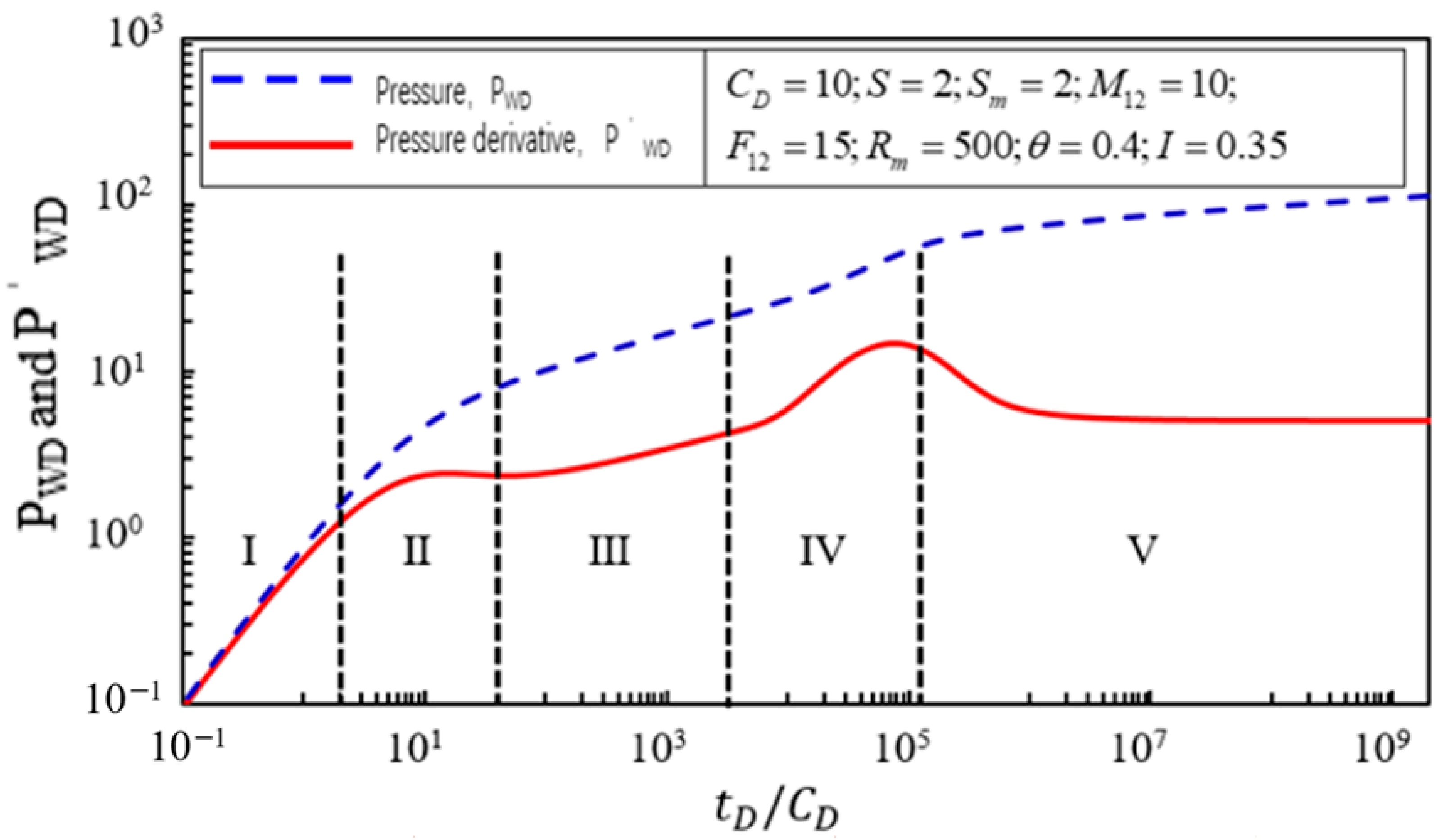
To analyze seepage characteristics during the initial stage of gas injection into an injection well, this section further employs the Stehfest numerical inversion technique to invert the solution of the bottom-hole pressure ${\overline{P}}_{WD}$ in Equation (47) under certain parameter conditions, as shown in Figure 3, and obtains dimensionless double-logarithmic bottom-hole pressure dynamic response characteristic curves for the initial real-space bottom-hole pressure $P_{WD}~t_D/C_D$ and $P_{WD}^{\text{'}}(t_D/C_D)~t_D/C_D$ for multicomponent gas injection into the injection well during the initial stage. Analysis of the research results shown in Figure 3 reveals that the typical curves for the pressure and pressure derivative can be divided into five seepage stages:

In the first stage, the wellbore storage controls seepage. The pressure derivative curve and pressure curve both exhibit straight lines with a slope of 1, and the two lines are coincident, passing through the origin.

In the second stage, this seepage segment is primarily controlled by the skin factor, showing an upward convex feature. Additionally, this seepage stage is also influenced in combination with the wellbore storage coefficient.

In the third stage, radial seepage of multicomponent water–gas in the transition region occurs. Due to the characteristic variation of the flow rate and storage coefficient of the multicomponent water–gas with radius, the pressure derivative curve shows a skewed line deviating from 0.5, with the slope of the line controlled by the storage coefficient and the power-law index ($\theta$, $I$) of the flow rate.

In the fourth stage, the transition of multicomponent water–gas from the transition region to the saline aquifer is mainly controlled by three parameters: the interface skin coefficient $S_m$, the ratio of the bottom of the well fluid flow rate to the saline aquifer $M_{12}$, and the ratio of the comprehensive storage coefficient of the fluid at the bottom of the well to the saline aquifer $F_{12}$. In this seepage segment, the pressure derivative curve exhibits an upward convex feature.

In the fifth stage, radial seepage of saline water into the saline aquifer occurs. The value of the pressure derivative curve is equal to 0.15 $M_{12}$ in a horizontal line, where $M_{12}$ represents the ratio flow rate of the fluid at the bottom of the well to the saline aquifer reservoir’s saline water flow rate.

4.2. Parameter Sensitivity Analysis

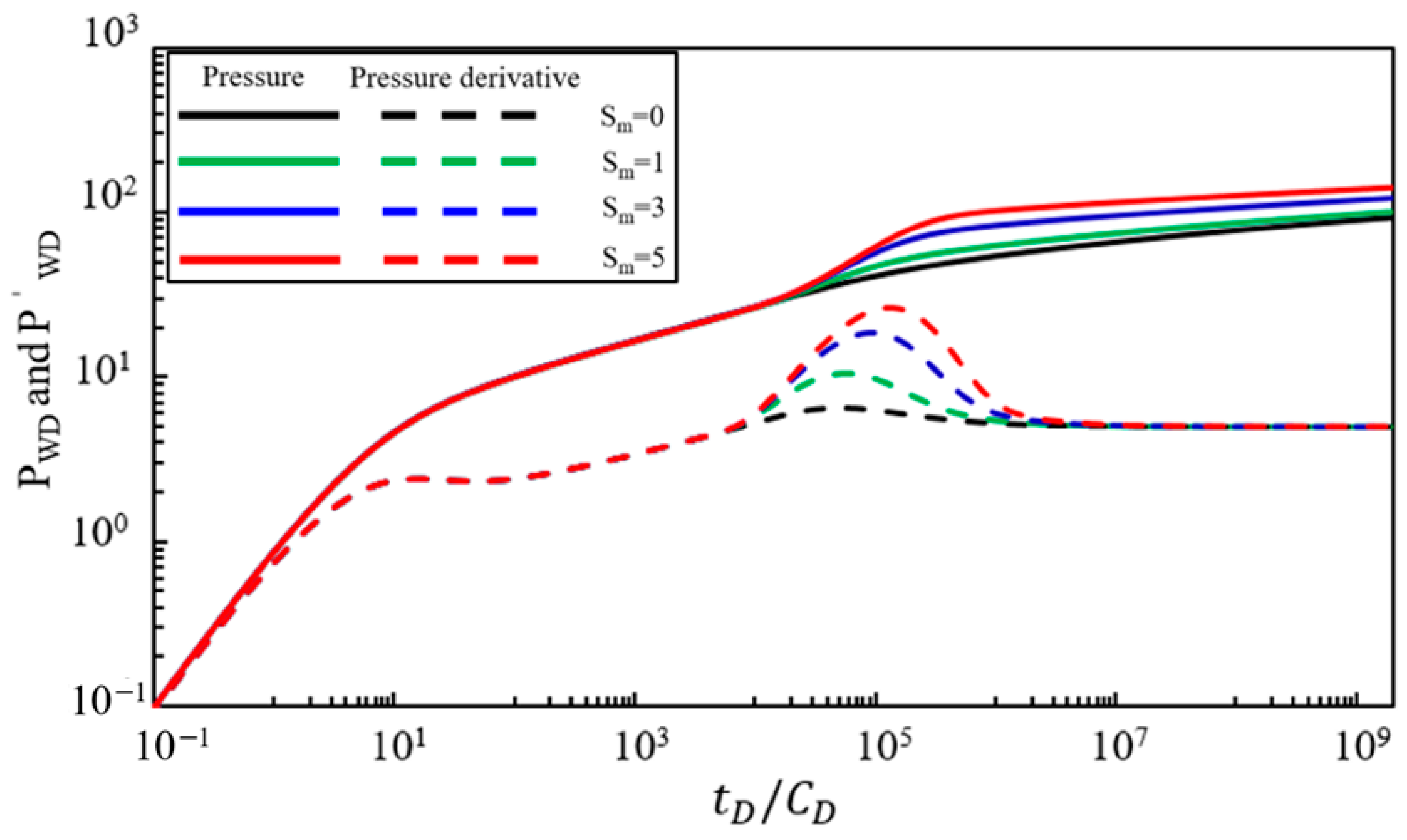
4.2.1. Saline Aquifer Interface Skin Coefficient

Figure 4 illustrates the effect of additional resistance at the interface between the multicomponent water–gas transition region and the saline aquifer on the dynamic bottom-hole pressure response. With other parameters held constant, the characteristic curves of the pressure and pressure derivative are calculated for the interface skin coefficient $S_m$ at 0, 1, 3, and 5. Analysis of the results in Figure 4 shows that the additional resistance at the transition region and at the saline aquifer interface primarily affects the third, fourth, and fifth flow stages. As the interface skin coefficient $S_m$ increases: (1) The straight line segments of the pressure derivative curve in the third and fifth flow stages become shorter. (2) The upward convexity of the pressure derivative curve during the transitional seepage stage significantly increases. Conversely, the smaller the interface skin coefficient $S_m$ is, the smaller the corresponding additional resistance at the interface is, resulting in a less pronounced upward convexity in the pressure derivative curve and a more gradual transitional seepage stage.

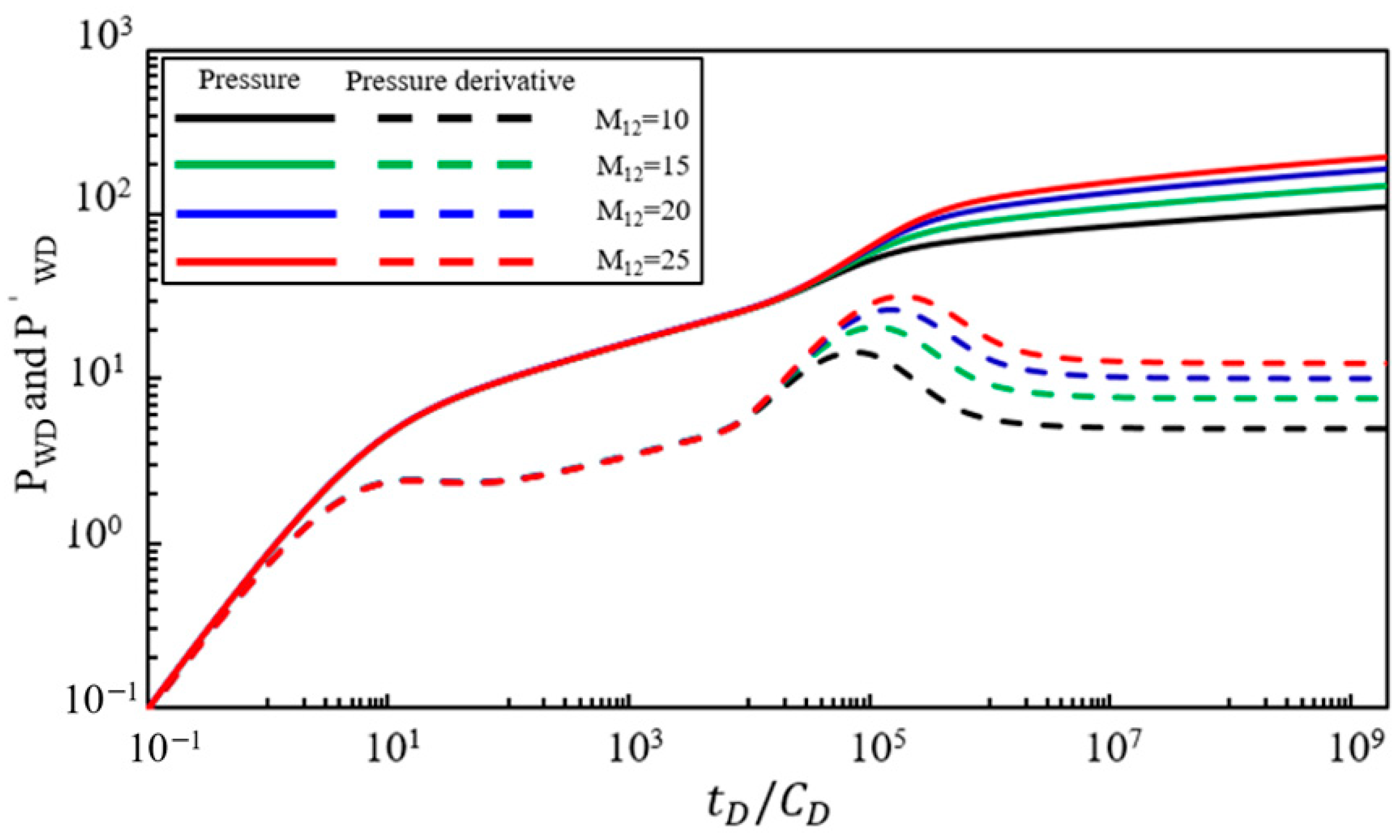
4.2.2. Fluid Mobility Ratio at the Bottom of the Well and at the Saline Aquifer Interface

Figure 5 shows the effect of the mobility ratio $M_{12}$ between the fluid at the bottom of the well and the saline aquifer on the dynamic bottom-hole pressure response. With other parameters held constant, the characteristic curves of pressure and pressure derivative are calculated for mobility ratios of 10, 15, 20, and 25. Analysis of Figure 5 indicates that the mobility ratio $M_{12}$ primarily affects the fourth and fifth flow stages. As the mobility ratio $M_{12}$ increases: (1) The pressure derivative value at the extremum points of the transition from the transition region to the saline aquifer (i.e., the fourth stage) increases. (2) The pressure derivative value at the horizontal segment during the radial flow in the saline aquifer (i.e., the fifth stage) increases. Conversely, as the mobility ratio $M_{12}$ decreases, the extremum points of the pressure derivative during the transition from the multicomponent water–gas transition region to the saline aquifer and the pressure derivative value during the radial flow in the saline aquifer decrease.

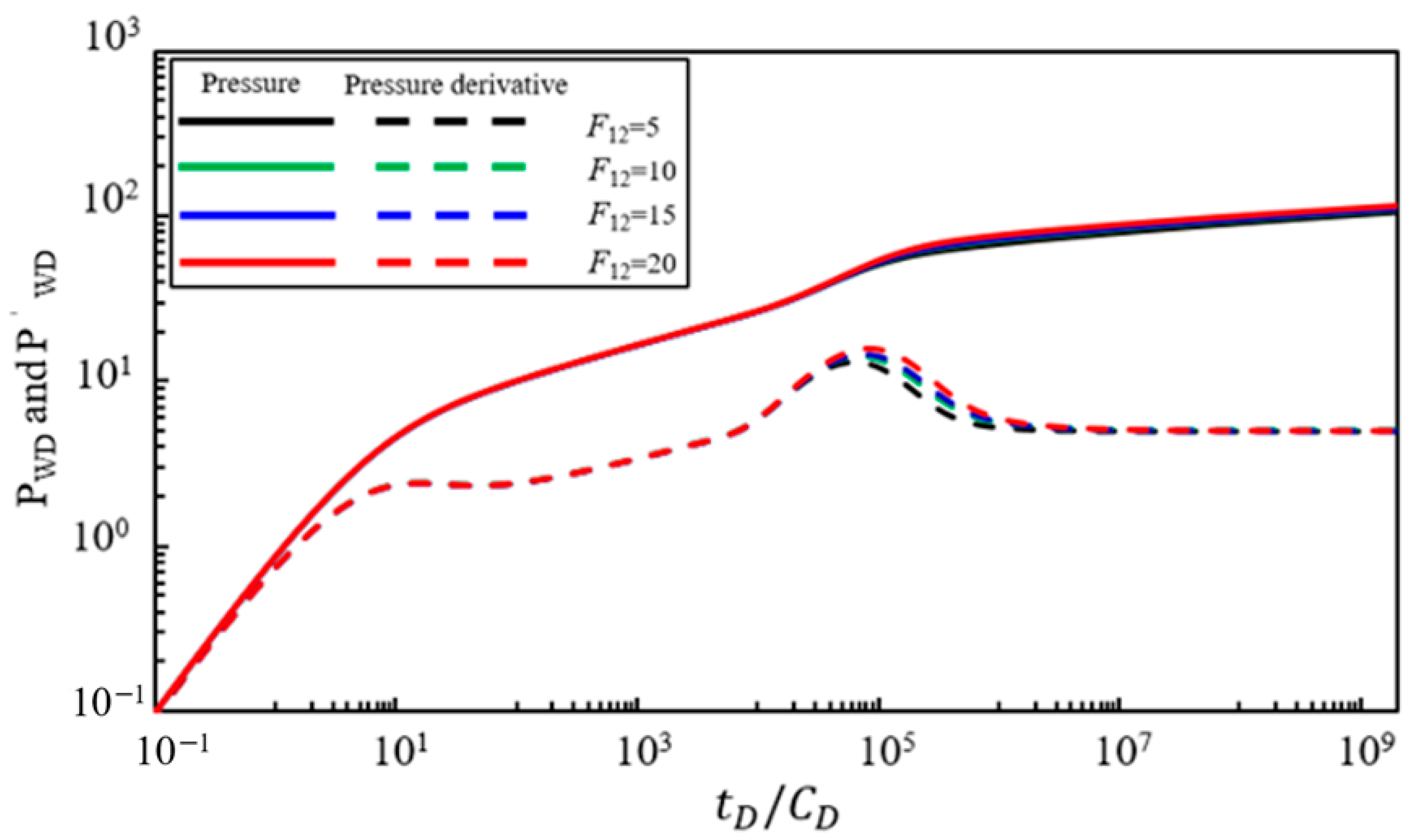
4.2.3. The Storage Capacity Ratio at the Interface between the Bottom of the Well Fluid and the Saline Aquifer

Figure 6 illustrates the effect of the storage capacity ratio $F_{12}$ at the interface between the fluid at the bottom of the well and the saline aquifer on the dynamic bottom-hole pressure response. With other parameters held constant, the characteristic curves for the pressure and pressure derivative are calculated for storage capacity ratios of 5, 10, 15, and 20. Analysis of Figure 6 indicates that the storage capacity ratio $F_{12}$ primarily affects the fourth and fifth flow stages. The influence of the storage capacity ratio $F_{12}$ is similar to that of the mobility ratio $M_{12}$. As the storage capacity ratio $F_{12}$ increases: (1) The extremum point during the transition from the transition region to the saline aquifer becomes larger. (2) The pressure derivative value during the radial flow in the saline aquifer does not show significant changes. Compared to the mobility ratio $M_{12}$, the effect of the storage capacity ratio $F_{12}$ on pressure derivative characteristics is notably weaker.

4.2.4. Radius of the Multicomponent Water–Gas Transition Region

Figure 7 illustrates the impact of the dimensionless radius $R_{mD}$ of the multicomponent water–gas transition region on bottom-hole pressure dynamics. Under constant conditions for other parameters, the pressure and pressure derivative characteristic curves are calculated for a dimensionless radius $R_{mD}$ of 100, 300, 500, and 700. Analysis of Figure 7 shows that the dimensionless radius $R_{mD}$ of the multicomponent water–gas transition region primarily affects the third, fourth, and fifth flow stages. As the dimensionless radius $R_{mD}$ increases: (1) The duration of the multicomponent water–gas’s radial flow extends. (2) The onset of radial flow in the saline region is delayed. (3) The transition flow stage from the transition region to the saline region occurs later.

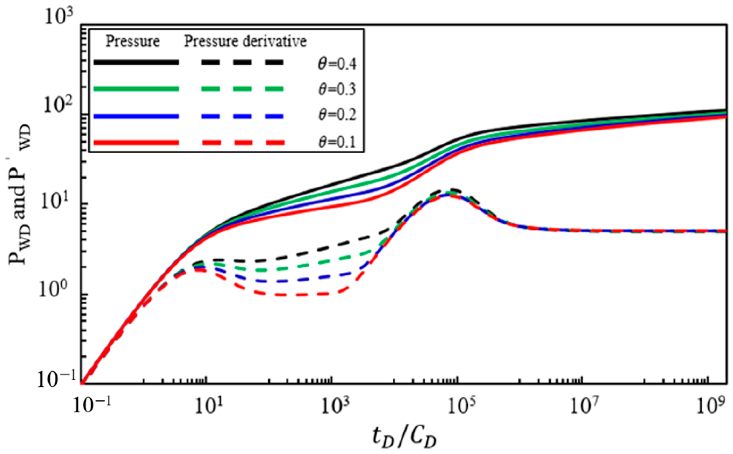
4.2.5. Power-Law Change Index of the Multicomponent Water–Gas Transition Region’s Mobility

Figure 8 shows the effect of the power-law change index $\theta$ of the multicomponent water–gas transition region’s mobility on bottom-hole pressure dynamics. When other parameters remain constant, the pressure and pressure derivative characteristic curves were calculated with a power-law change index $\theta$ of 0.4, 0.3, 0.2, and 0.1. Analysis of Figure 8 indicates that the power-law change index $\theta$ primarily affects the third and fourth flow stages. A larger power-law change index $\theta$ in the multicomponent water–gas transition region’s mobility was associated with the following: (1) A more significant upward slope in the multicomponent water–gas’s radial flow straight line characteristic segment, while the duration of the multicomponent water–gas’s radial flow in the transition region does not change significantly. (2) A slight increase in the peak pressure derivative value during the transitional flow stage between the transition region and the saline region.

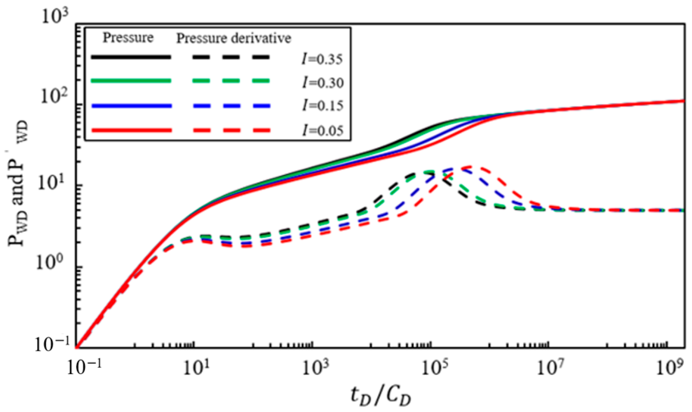
4.2.6. Power-Law Change Index of the Comprehensive Storage Capacity Coefficient of the Multicomponent Water–Gas in the Transition Region

Figure 9 illustrates the effect of the power-law change index $I$ of the comprehensive storage capacity coefficient of the multicomponent water–gas in the transition region on bottom-hole pressure dynamics. With other parameters held constant, the pressure and pressure derivative characteristic curves were calculated for $I$ values of 0.35, 0.30, 0.15, and 0.05. Analyzing Figure 9 reveals that the power-law change index $I$ primarily affects the third, fourth, and fifth flow stages. The following occurs as the value of $I$ increases: (1) the slope of the upward-tilting straight line segment of the multicomponent water–gas radial flow increases and (2) the duration of the multicomponent water–gas radial flow in the transition region does not significantly change. Compared to the power-law change index $\theta$ of the flow mobility, the impact of the storage capacity power-law change index $I$ on the slope of the multicomponent water–gas radial flow straight line segment is weaker.

4.2.7. Constant Pressure Boundary in the Outer Region

Figure 10 illustrates the effect of the outer region’s circular supply boundary $R_{eD}$ (constant pressure boundary) on the dynamic behavior of bottom-hole pressure. With other parameters held constant, the pressure and pressure derivative curves were calculated for constant pressure boundaries $R_{eD}$ of 20,000, 30,000, 40,000, and 50,000. Analysis of Figure 10 indicates that, under constant pressure boundary conditions, an additional late-time steady-state flow stage occurs compared to an infinite reservoir. In this flow stage, the pressure curve becomes a horizontal line, and the pressure derivative curve sharply decreases until it approaches zero. The outer constant pressure boundary $R_{eD}$ primarily affects the end time of the radial flow stage in the saline aquifer. A more significant constant pressure boundary $R_{eD}$ value results in a longer duration of radial flow in the saline aquifer, whereas a smaller $R_{eD}$ value leads to an earlier end to the radial flow stage.

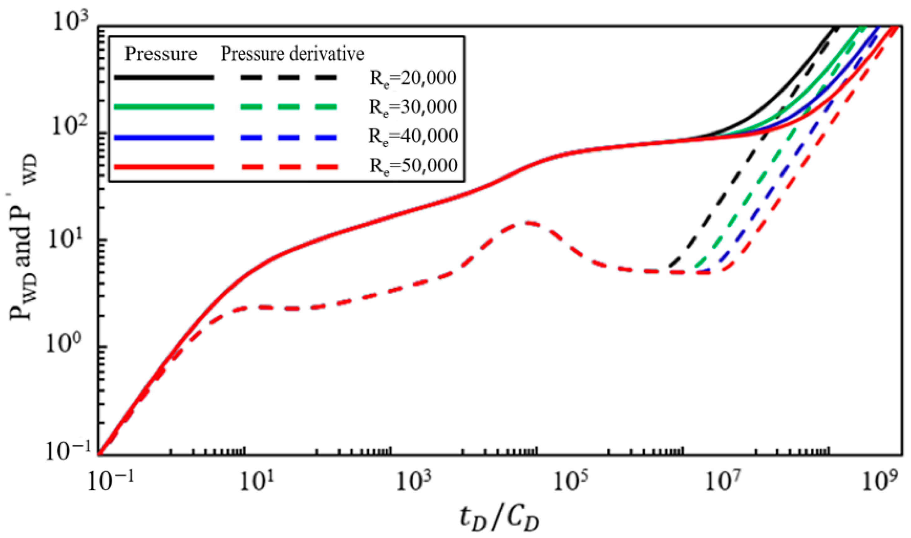
4.2.8. Closed Boundary in the Outer Region

Figure 11 illustrates the impact of the outer circular closed boundary $R_{eD}$ on bottom-hole pressure dynamics. With other parameters held constant, the pressure and pressure derivative characteristic curves are calculated for the closed boundar ${ R}_{eD}$ values of 20,000, 30,000, 40,000, and 50,000, respectively. Analysis of Figure 11 reveals that, similar to the constant pressure boundary, under closed boundary conditions, there is an additional late stable flow stage compared to the infinite reservoir. In this flow stage, both the pressure and pressure derivative curves become sharply rising straight lines with a slope of 45°. The outer closed boundary primarily affects the end time of radial flow in the saline region. A larger closed boundary $R_{eD}$ results in a longer duration of radial saline flow in the reservoir. Conversely, a smaller $R_{eD}$ value leads to an earlier end time for radial flow in the saline region.

Several parameters are mentioned in this paper, such as the interface skin coefficient and fluid mobility ratio. Although the sensitivity analysis provided is not comprehensive and does not explore in detail how these parameters affect the model output under different geological conditions to verify the model’s robustness, this approach helps to reduce computational complexity and improve efficiency, particularly in the early stages of preliminary model evaluation. By simplifying the sensitivity analysis of certain parameters, preliminary results can be obtained more quickly, providing a reference for subsequent, more detailed simulations and optimizations.

4.3. The Leakage Safety Discrimination

The CO₂ flow’s leading edge and leakage characteristics can be discriminated through Figure 4, Figure 5, Figure 6, Figure 7, Figure 8, Figure 9, Figure 10 and Figure 11. With different skin coefficients, fluidity ratios, and storage capacity ratios, the variation characteristics of the pressure derivative curves are different, and the CO₂ migration distance can be judged according to these characteristics. The boundary feature can determine whether CO₂ leakage occurs at the migration front. When the features in Figure 10 are present, this indicates that there is a leak, and when Figure 11 is present, it means that CO₂ is not leaking.

5. Conclusions

This study established and solved a leakage safety discrimination model for saline aquifer CCS based on pressure dynamics. The model results were further analyzed using Stehfest numerical inversion techniques to identify the influencing factors of various parameters. An in-depth analysis was conducted to investigate the nondimensional logarithmic dynamic response characteristic curves of the bottom-hole pressure under different parameter conditions.

5.1. Research Findings

(1) The pressure dynamic characteristics of the initial stage straight well testing model for gas injection wells were analyzed. The injection well testing curve in the initial stage of gas displacement is divided into five flow stages: a wellbore storage-controlled seepage stage, a skin-controlled seepage stage, a transitional radial seepage stage, a transitional seepage stage from the transitional region to the saline water region, and a saline water radial flow stage.

(2) The pressure dynamic characteristics of the later-stage straight well testing model for gas injection wells were analyzed. The injection well testing curve in the later stage of gas displacement is divided into seven flow stages: a wellbore storage-controlled seepage stage, a skin-controlled seepage stage, a radial seepage stage in the pure gas region, a transitional seepage stage between the pure gas region and the transitional region, a radial seepage of multicomponent water–gas in the transition region, a transitional seepage between the transitional region and the saline water region, and a saline region radial seepage stage.

(3) The dimensionless bottom-hole pressure and its derivative double-logarithmic theoretical well test curves were plotted for both the initial and late stages of the injection well’s straight well test models. Sensitivity analyses were also conducted on various parameters, including interface skin coefficients at different interface locations, the radius of each region, the fluid mobility ratios of each region, the ratios of each region’s storage coefficients, the fluid mobility ratios at interfaces, the ratios of storage coefficients at interfaces, the power-law change index of the multicomponent water–gas transition region’s mobility, the power-law change index of the comprehensive storage capacity coefficient of the multicomponent water–gas, and the boundary conditions. This yielded influence factor charts for the injection well test curves at different development stages.

(4) Through the typical curves of the pressure and pressure derivatives from the composite injection well tests in the initial radial stages of gas displacement, it is evident that the typical curves can be divided into five flow stages. Notably, the fourth stage reveals that, during the transition of the multicomponent gas from the transition region to the saline water region, the main controlling factors are the interface skin coefficient $S_m$, the fluid mobility ratio at the bottom of the well and saline aquifer interface $M_{12}$, and the ratio of the comprehensive storage coefficient of the fluid at the bottom of the well to the saline aquifer $F_{12}$. In this flow segment, the pressure derivative curve exhibits a characteristic convex shape.

5.2. Future Prospects

(1) The parameters that primarily influence the bottom-hole pressure ${\overline{P}}_{WD}$ include: the saline aquifer interface skin coefficient, the fluid mobility ratio at the bottom of the well and the saline aquifer interface, the storage capacity ratio at the interface between the fluid at the bottom of the well and the saline aquifer, the radius of the multicomponent water–gas transition region, the power-law change index of the multicomponent water–gas transition region’s mobility, the power-law change index of the comprehensive storage capacity coefficient of the multicomponent water–gas in the transition region, the constant pressure boundary in the outer region, and the closed boundary in the outer region. In the future, the bottom-hold pressure’s curve characteristics can be analyzed based on these parameters.

(2) This article predicts the leakage of CO₂ in saline water layers through pressure dynamics, which can serve as a model for future practical models, and the pressure and its reciprocal curve can reflect the flow of CO₂ in the formation.