Article

Simulation of Plastic Deformation Failure of Tillage Tools Based on the Smoothed Particle Hydrodynamics Method

1
College of Engineering and Technology, Southwest University, Chongqing 400715, China
2
Chongqing Chang’an Technology Co., Ltd., Chongqing 400023, China
*
Author to whom correspondence should be addressed.
Processes 2024, 12(1), 86; https://doi.org/10.3390/pr12010086
Submission received: 11 December 2023 / Revised: 25 December 2023 / Accepted: 27 December 2023 / Published: 29 December 2023

Abstract

:
The problems of large deformations, failures, and fractures that agricultural tillage tools may encounter during the cultivation process has long been a concern in the field of agricultural machinery design and manufacturing. It is important to establish a more accurate numerical model to effectively predict tools’ plastic deformation failures and ductile fracture failures. This research develops a numerical model for predicting the plastic deformation failure and ductile fracture failure of agricultural tillage tools using the smoothed particle hydrodynamics (SPH) method and the Johnson–Cook constitutive model. The model uses the Drucker–Prager criterion to describe the elastic–plastic constitutive behavior of the soil, the von Mises criterion to describe the Johnson–Cook constitutive model of the tool, and the coupling condition with the Lennard-Jones repulsive force to describe the interaction between the tool and soil. The numerical results show that the proposed model can effectively simulate the interaction between the tool and soil, as well as the tool’s plastic deformation failure and ductile fracture failure during the agricultural cultivation process. It can also predict the variation trend of the cutting force of the tool. This helps to provide a new approach for the numerical simulation of such problems.

1. Introduction

Agricultural tillage tools (such as plowshares, subsoilers, disc harrows, rotary blades, etc.) [1] may encounter plastic deformation failure and ductile fracture failure during cultivation operations, especially in regions with poor soil conditions (such as the rocky and sticky soil in mountainous areas, where the probability of tool failure is high) [2]. Assessing and predicting the likelihood of plastic deformation failure and ductile fracture failure in agricultural tillage tools and evaluating the tool–soil interaction during agricultural tillage operations has always been a challenging issue in agricultural tillage tool research. This is because the condition of the tillage tool directly affects the reliability and efficiency of the overall tillage machinery operation as a key component [3,4]. Therefore, establishing a reliable mechanical model to study the cutting process and the potential large deformation failures of the tool would be beneficial. Such a model could assist in optimizing tool design and reducing the failure rate of tillage machinery.
Currently, research on agricultural tillage tools primarily includes two approaches: field experiments and numerical simulations. Field experiments are the major approach used for designing and studying agricultural tillage tools [5]. However, field experiments are limited to studying the cutting process and tool conditions using external macroscopic morphology and measurements. This makes it difficult to reflect the dynamic mechanism arising from the internal structure of the tool and soil through field experiments alone. Additionally, conducting comprehensive field experiments can be time-consuming and laborious [6]. With the rapid development of computer technology and numerical methods, simulating the dynamic responses of the tool and soil through numerical methods has become an effective approach to studying tool–soil interactions, which facilitates research into tool optimization, failure prediction, and tillage strategy [4].
In the study of tillage tool–soil interactions in the agricultural field, tools are typically simplified and modeled as either rigid or deformable bodies. Currently, the assumption of tool rigidity is more widely used. This simplification does not consider tool deformation, greatly reducing the modeling and computational complexity [7,8,9,10,11,12,13]. For example, Yang et al. [14] simulated the soil-cutting process using the finite element method (FEM) and studied the cutting force under different parameters, such as tool rake angles, tillage depths, and friction coefficients; however, they did not model tool deformation. Similarly, Fang et al. [15] verified a discrete element method (DEM) tool–soil interaction model by establishing an experimental setup and analyzing the changes in the resultant force, horizontal force, and vertical force of the rotary blade; this also assumed the tool to be a rigid body. Gao et al. [7] developed a soil–tool interaction model based on SPH, verified the accuracy of the soil–tool interaction model; they also assumed a rigid tool. In recent years, some researchers have started to model tools as deformable bodies using multi-physics joint simulations, obtaining information such as tool stress and deformation. However, this approach requires significant computational resources compared with the assumption of rigidity. Zhang et al. [16] conducted FEM studies on the maximum stress value, maximum total deformation, and minimum fatigue life of a rotary blade. The simulation results agreed with the actual conditions, verifying the feasibility of FEM simulations for small deformations of tools. Zhang et al. [17], focusing on the easy wear failure problem of soil-engaging components in agricultural machinery, used DEM and FEM for a combined simulation. They obtained parameters such as the average deformation and equivalent stress after a sample wear test, further evaluating the wear characteristics and exploring the wear-resistance mechanism.
In general, the aforementioned methods can simulate the cultivation process and analyze tool forces to a certain extent. However, simulating large or fracturing deformations under certain scenarios remains difficult, especially when trying to predict failure by considering tools as deformable bodies with material properties. The classic FEM is prone to numerical divergence caused by mesh distortion when processing large deformations [4]. DEM can simulate large deformation problems, but it is more suitable for materials with non-cohesive soil particles, and the calibration of soil parameters is complicated [18]. Some coupled methods require continuous updating of the grid during the calculation process. As a meshless method, the SPH method, with its superior adaptivity, allows the solution process to remain unaffected by the randomness of particle distribution; this can handle extremely large deformation problems well. It also has a wide range of applications in solving highly nonlinear problems such as high-speed collisions and explosions [13]. Therefore, the SPH method has good potential for modeling deformable tool–soil interactions.
This paper establishes a coupled numerical model based on the smoothed particle hydrodynamics (SPH) method, to consider the interaction between deformable tools and soil. The model utilizes the Drucker–Prager constitutive relation to describe the elastoplastic deformation behavior of the soil. It also implements the Johnson–Cook constitutive model to characterize the progressive plastic deformation and fracture evolution of the tool under loading. Through simulation and analysis, the model is found to accurately predict the nonlinear tool–soil interaction as well as the complex plastic deformation and fracture processes in the tool. Compared with traditional methods assuming rigid tools, this coupled model can more accurately describe the nonlinear tool–soil interaction and complex deformation mechanisms that occur. By accounting for large deformations and potential failure modes, this study provides a new perspective for the optimization design of agricultural equipment and tools.

2. Simulation Approaches

2.1. The Basics of SPH Method

The basic idea of SPH can be summarized as follows: use a group of particles with physical properties to discretize the problem domain, approximate the governing equations of the fluid to the form of the ordinary differential SPH equations, and solve these using the weighted averages of the particles in the support domain to obtain the desired physical quantities. There are two key steps in the construction of the SPH equation: kernel function approximation and particle approximation.

2.1.1. Kernel Function Approximation

The integral expression of the function f(x) at point x in the problem domain Ω is defined as
f ( x ) = Ω f ( x ) δ ( x x ) d x
where δ ( x x ) is the Dirac function:
δ ( x x ) = f ( x ) = { ,     x = x 0 ,     x x
By replacing the Dirac function with a smoothing kernel function, the expression of the h kernel function can be approximated as
f ( x ) = Ω f ( x ) W ( x x , h ) d x
In this equation, W ( x x , h ) represents the smoothing kernel function; h is the smooth length, which is used to define the influence of the smoothing kernel function [19]. This study selects the cubic spline smoothing function [20] as the kernel function for SPH research:
W ( R , h ) = α d × { 2 3 R 2 + 1 2 R 3 ,     0 R < 1 1 6 ( 2 R ) 3 ,                                   1 R < 2 0 ,                                                       R 2
In this equation, R = | x   -   x | / h , for two-dimensional spaces, and α d takes values of 15/(7 π h2).

2.1.2. Particle Approximation

The particle approximation discretizes the problem domain into a finite number of particles with independent spaces. The field variable on each particle can be obtained by summing the weighted field variables of all neighboring particles within the support domain [21]. In the SPH method, the volume of particle j is represented by using the volume Δ V j to replace the infinitesimal element dx in Equation (3); thus, it can be expressed as [19]
Δ V j = m j / ρ j
In this equation, m j is the mass of particle j (j = 1, 2, …, N), where N is the total number of particles within the support domain of particle j; ρ j is the density of particle j [19]. Substituting Equation (5) into Equation (3) yields an approximate equation for particle i:
f ( x i ) = j = 1 N m j ρ j f ( x j ) · W ( x i x j , h )
In this equation, x i and x j represent the respective position function variables of particle i and particle j.

2.2. Discretization of Governing Equations

The mass conservation equation in the Navier–Stokes equations under the SPH method is
ρ i = j = 1 N m j W i j j = 1 N m j ρ j W i j
The momentum conservation equation in the Navier–Stokes equations under the SPH method is
D v i α D t = j = 1 N m j ( σ i α β ρ i 2 + σ j α β ρ j 2 ) W i j x i β + f α
The energy conservation equation in the Navier–Stokes equations under the SPH method is
D e i D t = 1 2 j = 1 N m j ( P i + P j ρ i ρ j ) v i j β W i j x i β + μ i 2 ρ i ε i α β ε j α β
In the equation, v represents velocity, e represents internal energy, σ represents the stress tensor, P represents pressure, m represents mass, ρ represents density, μ represents the dynamic viscosity coefficient, ε represents the strain rate, N represents the total number of particles within the support domain, x represents the particle coordinate position, and α   and   β denote Cartesian components; i and j represent different particles.
In order to avoid the issues of stress instability and nonphysical oscillations in traditional SPH methods [22], the widely used artificial stress term K i j and artificial viscosity term Π i j [23] are employed in the solution. The momentum from Equation (8) is modified as
D v i α D t = j = 1 N m j ( σ i α β ρ i 2 + σ j α β ρ j 2 + K i j + Π i j ) W i j x i β + f α

2.3. Constitutive Model of the Soil

The soil particle stress rate equation in the SPH form is constructed based on an elastoplastic constitutive model adopting the Drucker–Prager (D–P) yield criterion for soil particles:
D σ i α β D t = σ i α γ ω ˙ i β γ + σ i γ β ω ˙ i α γ + 2 G e ˙ i α β + K ε ˙ i γ γ δ ˙ i α β λ ˙ i [ 9 K sin ψ δ α β + G J 2 s i α β ]
In this equation, the first two terms are the Jaumann stress rate [23], ε ˙ α β represents the strain rate tensor, ω ˙ α β represents the rotation rate tensor, and λ ˙ i represents the plastic multiplier; these are defined as
ε ˙ i α β = 1 2 [ j = 1 N m j ρ j ( v j α v i α ) W i j x i β + j = 1 N m j ρ j ( v j β v i β ) W i j x i α ]
ω ˙ i α β = 1 2 [ j = 1 N m j ρ j ( v j α v i α ) W i j x i β j = 1 N m j ρ j ( v j β v i β ) W i j x i α ]
λ ˙ i = 3 α ϕ K ε ˙ i γ γ + ( G / J 2 ) s i α β ε ˙ i α β 27 α ϕ K sin ψ + G

2.4. Constitutive Model of the Cutting Tool

The total stress tensor σ α β in Equation (10) is composed of the volumetric pressure P and the deviatoric shear stress τ α β :
σ α β = P δ α β + τ α β
By substituting Equation (15) into Equation (10), we obtain
D v i α D t = j = 1 N m j [ ( P i ρ i 2 + P j ρ j 2 ) δ α β + ( τ i α β ρ i 2 + τ j α β ρ j 2 ) + K i j + Π i j ] W i j x i β + f α

2.4.1. Equation of State

The volumetric pressure P of the tool in Equation (16) is calculated using the equation of state, as
P = ρ 0 C 0 2 η [ 1 + ( 1 Γ 0 2 ) η ] [ 1 ( S a   1 ) η ] + ρ 0 Γ 0 e
In this equation, η = ρ ρ 0   -   1 , Γ 0 is the Gruneisen’s constant, S a is a linear Hugoniot slope coefficient, and e is the internal energy per unit of mass.

2.4.2. von Mises Yield Criterion

The shear stress τ of elastic solids can be obtained from
d τ i α β d t = τ i α γ ω ˙ i β γ + τ i γ β ω ˙ i α γ + 2 G ( ε ˙ i α β 1 3 δ α β ε ˙ i γ γ )
In this equation, G represents the shear modulus of the material, ε ˙ α β denotes the strain rate tensor, and ω ˙ α β represents the rotation rate tensor, as shown in Equations (12) and (13).
According to [24], based on the von Mises yield criterion, the aforementioned elastic constitutive relationship can be extended to plastic behavior:
f y = σ y 3 J 2
In this equation, σ y represents the yield stress, and J 2 denotes the second stress tensor invariant. When the von Mises yield criterion is satisfied ( f y   <   1 ), the material is in the plastic state; then, the shear stress is brought back to the yield surface. The shear stress τ α β at this point is
τ α β = f y τ α β

2.4.3. Johnson–Cook Constitutive Model

The Johnson–Cook constitutive model can describe the plastic deformation behavior of metals under conditions of large deformations, high strain rates, and elevated temperatures [25]. In this study, the Johnson–Cook constitutive model is selected as the material model for the cutting tool, where the yield stress of this constitutive model is represented as
σ y = [ A + B ( ε e f f p ) N ] [ 1 + C l n ( ε e f f p ˙ ε 0 ˙ ) ] [ 1 ( T * ) M ]
In this equation, ε eff p ( =   ε eff p ˙ d t ) represents the equivalent plastic strain; ε ˙ e f f p ( = 2 3 ε ˙ α β ε ˙ α β ) represents the equivalent plastic strain rate; ε 0 ˙ represents the reference value of the equivalent plastic strain rate; A, B, C, N, and M are constants related to the material; and T * represents the normalized temperature [24]:
T * = T T r e f T m e l t T r e f
In this equation, T r e f represents the reference temperature and T m e l t represents the melting temperature of the corresponding material.
The Johnson–Cook constitutive model can be combined with progressive damage and failure models to specify different damage initiation criteria and damage evolution laws, to demonstrate the phenomenon of fracture [25].
The progressive damage and failure criterion is employed to simulate the influence of tool deformation failure. Parameter D is used to measure the local damage state, as
D =   Δ ϵ e f f p ϵ f a i l u r e
In this equation, Δ ε e f f p represents the increment of equivalent plastic strain that occurs within an integration cycle, and ε f a i l u r e denotes the failure strain:
ε f a i l u r e = [ D 1 + D 2 exp ( D 3 σ * ] [ 1 + D 4 ln ( ε e f f p ˙ ε 0 ˙ ) ] [ 1 + D 5 T * ]
When the parameter D in Equation (23) exceeds 1 for particle i, a material failure occurs and the corresponding shear stress at point i is set to zero [24].

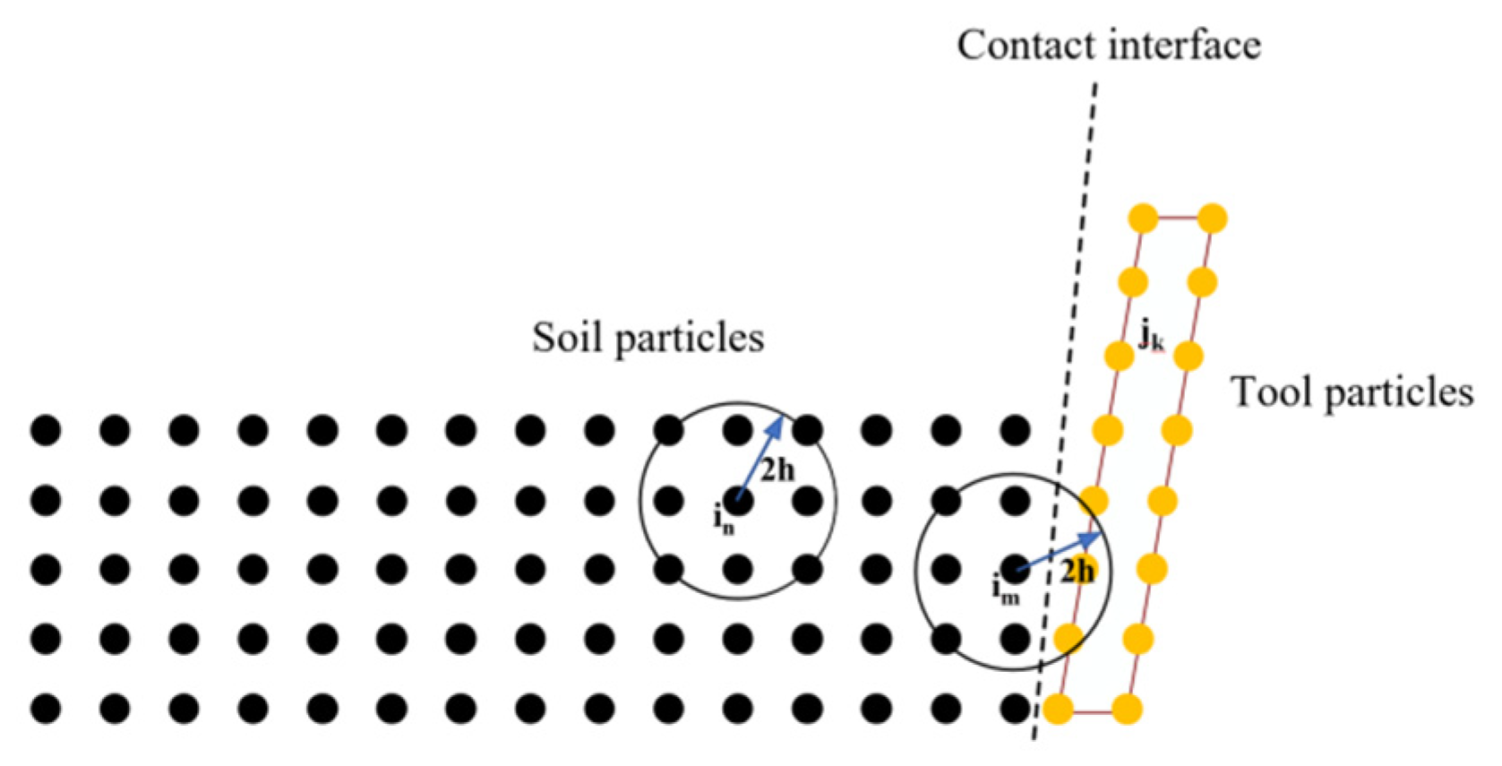
2.5. Tool–Soil Interaction Model

This paper introduces a cutting tool–soil interaction model that employs the soil–solid interface coupling condition [26], which satisfies the following conditions for each particle located at the interface:
v s o i l α = v s o l i d α
σ s o i l α β = σ s o l i d α β
To satisfy the conditions above, particles near the cutting tool–soil interface should meet the following requirements: During the SPH particle weighted summation process, for all particles within a distance of 2 h from the interface, we should neglect the differences in particle types (i.e., soil particles and tool particles), as shown in Figure 1. In other words, the velocity tensors and stress tensors of the tool particles can be applied to the soil particles through a smoothing function, and vice versa [26].
To prevent mutual penetration between the soil and tool particles, a penalty force similar to the Lennard-Jones repulsive force [27] is applied to them when particles of different materials approach each other near the interface.

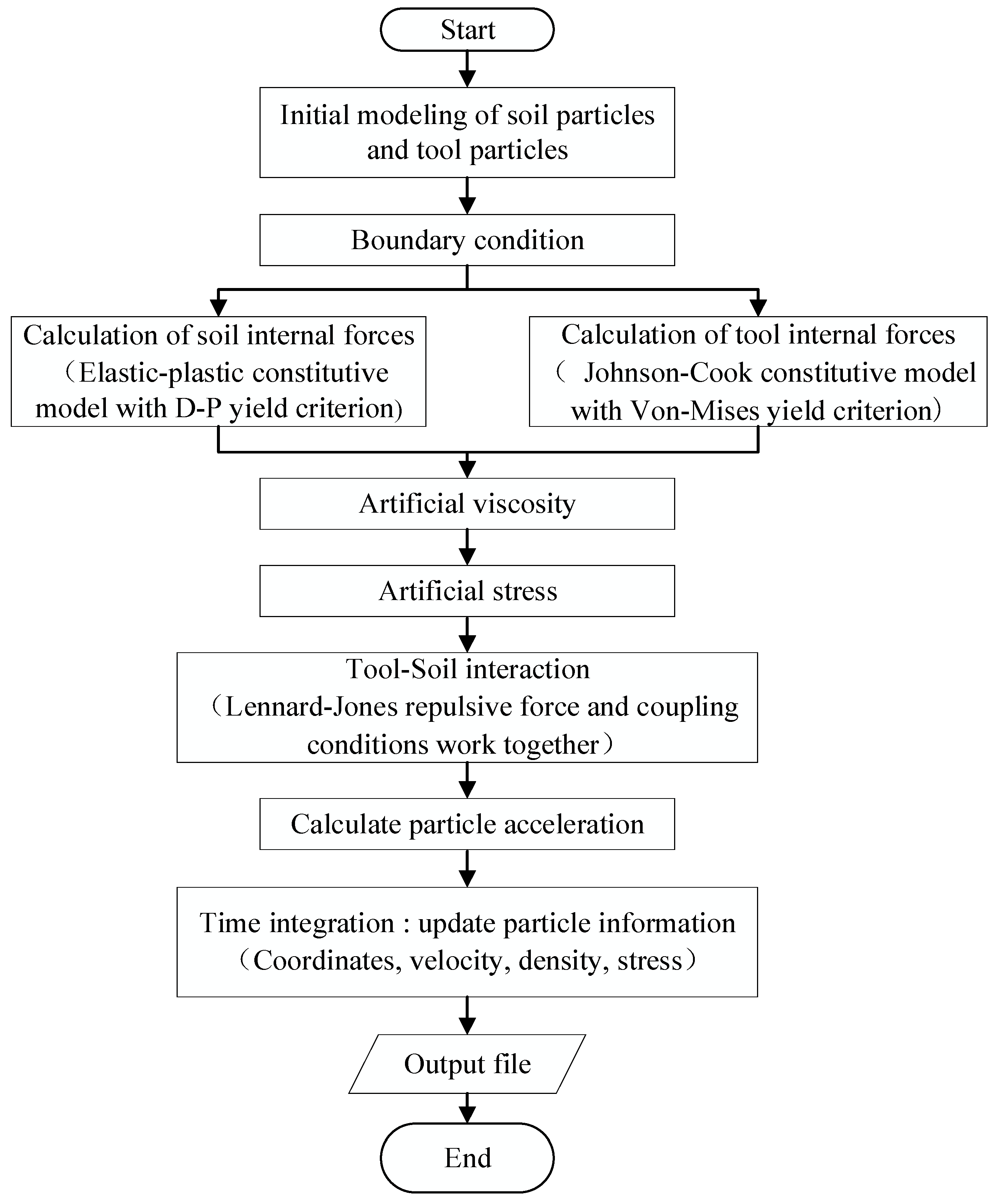
2.6. Model Implementation Process

Based on the above theory, this paper uses Fortran to write an SPH program for numerical computation of the tool-cutting process. The implementation process of the program is shown in Figure 2. The main task in establishing the initial model is to write the initial coordinates, density, velocity, and force conditions of soil particles and tool particles. Then, using the elastic–plastic constitutive model and the Johnson–Cook constitutive model, and combining them with a series of numerical processing methods, the internal force parameters of soil particles and tool particles are calculated separately, and the interaction is solved by coupling conditions. Finally, using temporal integration, the particle information is updated, and the desired data are outputted.

3. Numerical Example and Result Analysis

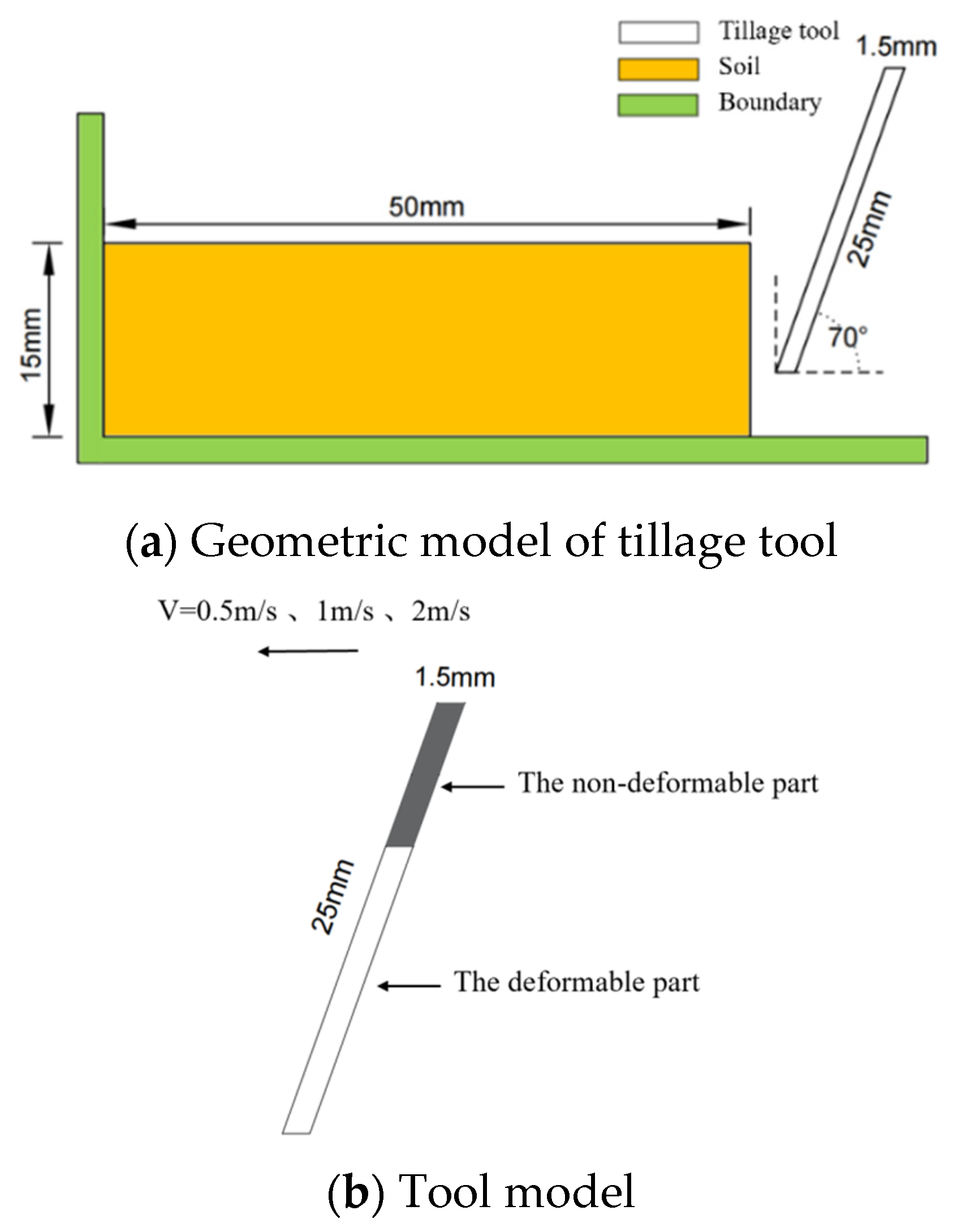
3.1. Model Construction and Parameter Setting

This paper establishes a two-dimensional numerical model to study the progressive deformation and fracturing behavior of tillage tools under different representative working conditions. As depicted in Figure 3a, the proposed model consists of a deformable tillage tool tilling a simplified rectangular soil domain. The tillage tool is modeled with dimensions of length 25 mm and thickness 1.5 mm, and it tills the soil at an angle of 70° to a depth of 10 mm. To enable clear observations of the dynamic cutting process, the tillage tool is modeled using a relatively soft aluminum alloy rather than the wear-resistant steels commonly utilized in actual tillage operations. While unrealistic in terms of material properties, the use of a lower-strength aluminum alloy serves to amplify the progressive deformation response and ductile fracture characteristics of the tillage tool, providing more prominent visualizations of the tool’s behavior. The soil domain is modeled as a simple fixed rectangular region with dimensions of length 50 mm and height 15 mm and is discretized into a network of uniformly spaced particles with a spacing of 1 mm between particles. This provides an appropriate balance between computational efficiency and solution accuracy. Typical parameters for a representative cohesive agricultural soil are utilized, accounting for plasticity and cohesion. The thermodynamic and damage parameters for the aluminum alloy are also selected to accurately characterize the material’s progressive ductile deformation and fracture behavior under the complex loading imparted by the soil-cutting process. As summarized in Table 1, the representative properties of the soil and aluminum tool enable comprehensive studies of the tool’s performance and soil interactions under typical loading conditions relevant to agricultural applications. By incorporating a deformable tool and characterizing the progressive damage, this model provides enhanced capabilities beyond the traditional rigid tool assumptions used to study tool fracture failures.

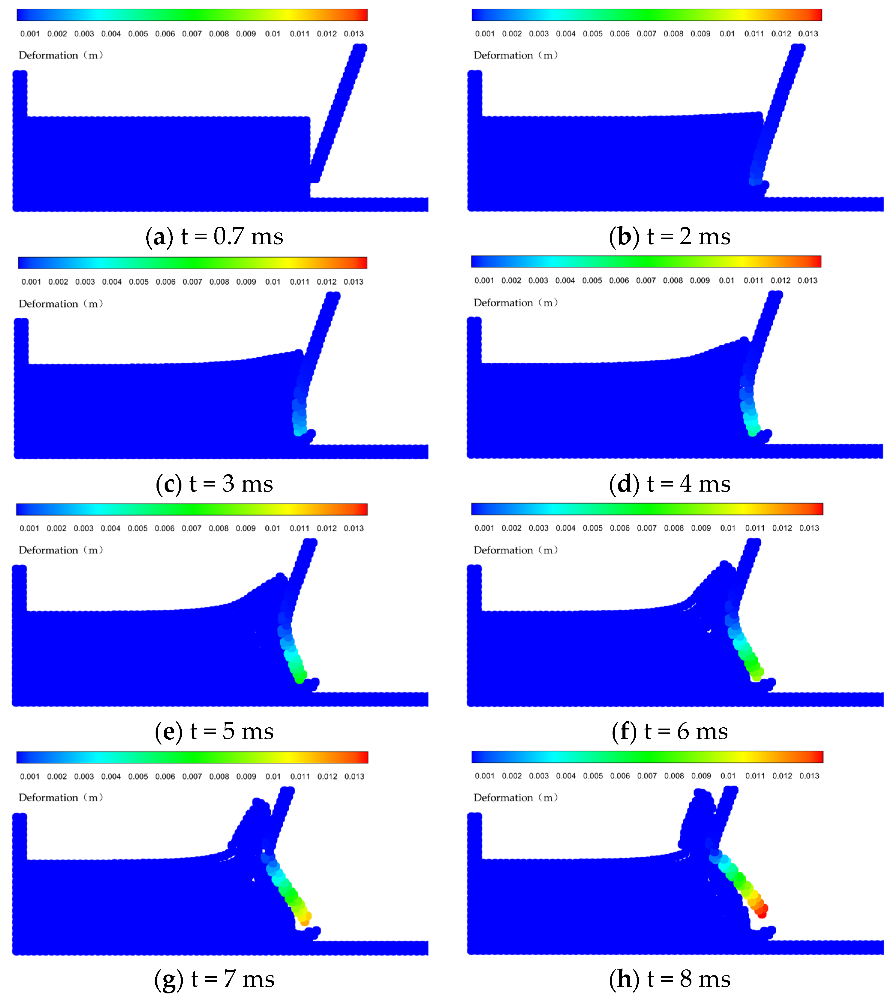
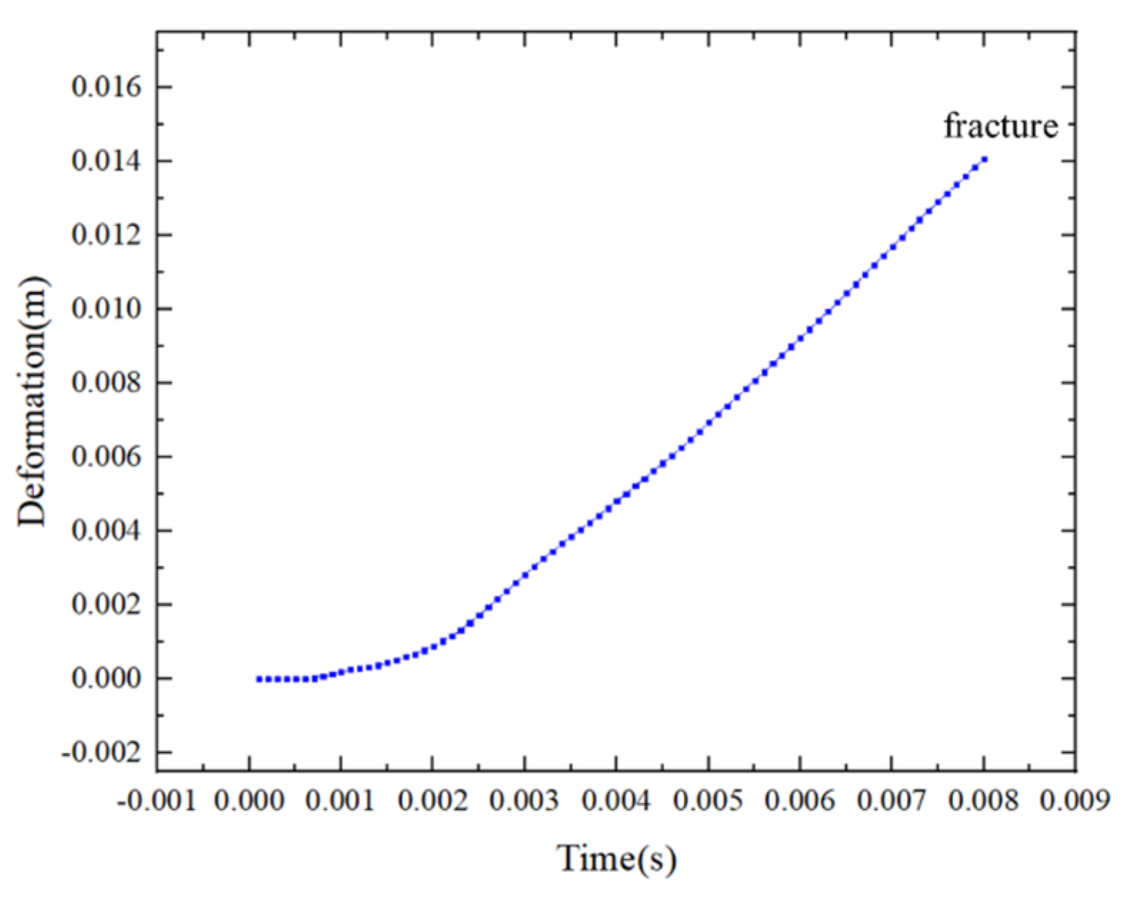
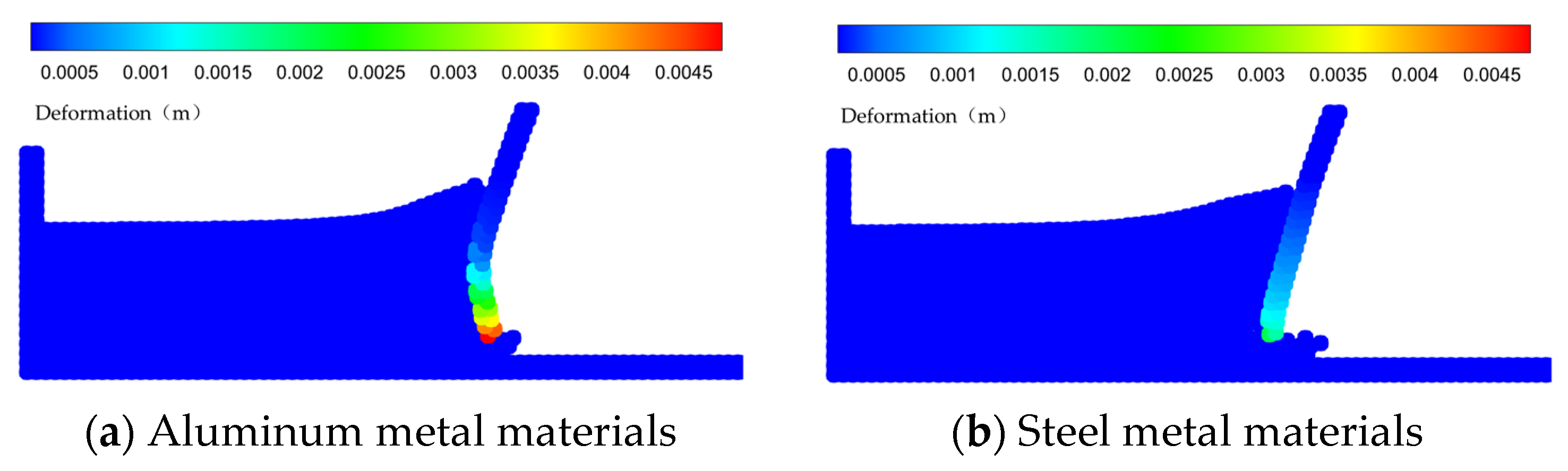
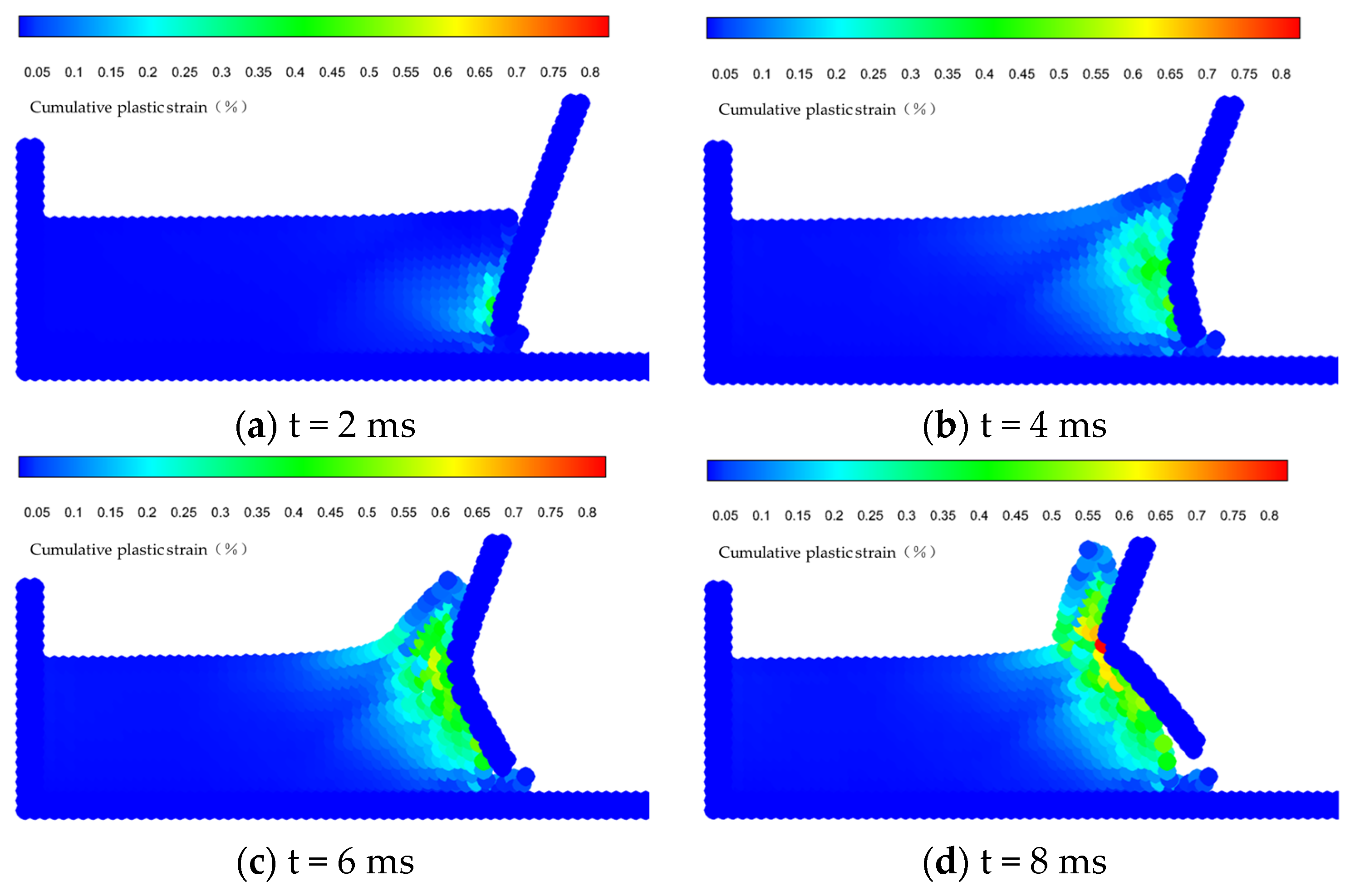
3.2. Process of Tool Deformation and Fracture

This study utilizes numerical simulations to investigate the progressive development of deformation and the eventual ductile fracture failure of agricultural tillage tools under representative loading conditions. A virtual cultivation environment is established consisting of a simplified tillage tool cutting through a rectangular soil domain at a constant speed. As depicted in Figure 3b, the upper section of the tool is modeled as a non-deformable body that moves horizontally from right to left at a defined speed of 2 m/s. The lower cutting section of the tool is deformable and follows the motion of the rigid upper section. This setup aims to provide enhanced insights into the full progressive failure process, from initial elastic response through extensive plastic deformation to eventual fracture.
Initially, the front tip of the tool experiences minor elastic strains due to the cutting resistance concentrated at the leading end. As the tool advances further into the soil, the contact region between the tool and the soil gradually grows larger, resulting in the development of substantial plastic deformation along the lower portion of the tillage tool. The plastic zone expands to encompass the entire tool length, at which point the tool enters a plastic strengthening stage. Here, the deformation sharply escalates as the tool is subjected to increasing loads over larger contact areas. Ultimately, the excessive accumulated plastic strain exceeds the ductility limit of the tool material, leading to crack initiation and propagation. The virtual model enables close examination of how the ductile fracture process evolves from localized elastic strains to extensive plastic flows, culminating in catastrophic failure crack formation. By simulating the comprehensive interactive behavior between the deformable tool and soil medium, the model captures the continuous evolution of the tool’s deformation and damage response under representative loading conditions relevant to agricultural applications. The results illustrate the mechanisms leading to fracture failure from initial cutting resistance, offering an effective platform to study agricultural tool fracture and optimize tool designs.
Figure 4 provides a detailed visualization of the progressive development of deformation and eventual ductile fracture failure of the agricultural tillage tool throughout the simulated dynamic cutting process. Figure 4a shows the initial undeformed configuration of the tool as it first makes contact with the pristine soil medium prior to any cutting. The sequence in Figure 4b through to Figure 4h then demonstrates the continuous evolution of the tool’s deformation response over time as it interacts with the soil during the advancing cutting motion. These simulation results enable extensive analysis of the full progressive damage process leading to fracture of the tool. Specifically, Figure 4b reveals that minor localized elastic strain is first concentrated at the front tip of the tool at t = 2 ms after the initial soil contact. As cutting continues, Figure 4c through to Figure 4h show the tool deforming extensively due to the increasing soil resistance forces along the cutting interface. The accumulated soil build-up applies escalating loads along the surface of the tool. This leads to a transition from the initial localized elastic response at the tip to a substantial plastic flow extending across much of the tool length. The large plastic deformation culminates in ductile overload fracture, as shown in the final Figure 4h. By capturing the comprehensive interactive behavior, these detailed simulation visualizations provide unique insights into the complex transition from elastic deformation to extensive ductile damage. The model enables a thorough examination of the mechanisms by which increasing soil cutting forces first lead to reversible elastic strains, followed by the progressive development of severe plastic deformation that ultimately precipitates catastrophic fracture failure. This understanding of the complete failure sequence under representative loading facilitates the optimization of agricultural tillage tools to improve robustness and fracture resistance.
The deformation at the front tip of the tool is more obvious, and Figure 5 illustrates the deformation pattern here. In the early stage of tool deformation, the soil and tool contact area is small, and the cutting resistance is also small, so the front tip of the tool is not significantly deformed. As the contact area increases, the cutting resistance grows and the deformation at the front tip of the tool is similar to a linear change before fracture. The deformation pattern can provide a more accurate supplement as well as a reference for improving the robustness and fracture resistance of agricultural tillage tools.
To further investigate the tool’s resistance to deformation under loading, this study conducts comparative simulations utilizing tool models with varying mechanical properties. Specifically, the deformation response is analyzed for tools modeled with both aluminum alloy and steel materials exposed to identical simulated cutting conditions. The simulation results clearly demonstrate that the steel tool exhibits a substantially enhanced resistance to plastic deformation compared to the relatively softer aluminum tool, as shown by the deformation patterns in Figure 6. Under the same applied loads, the aluminum tool experiences more extensive plastic flow, while the steel tool is better able to withstand the forces with higher strength and hardness, resulting in reduced strains.
Quantitatively, the maximum deformation in the aluminum tool reached over 4.8 mm before failure, while the steel tool only deformed by approximately 1.9 mm plastically. This difference highlights the importance of material strength and hardness in avoiding excessive plastic damage and improving robustness against deformation and fracture failure. This comparative study provides an effective platform for evaluating tool materials and optimizing material selection to withstand anticipated cutting loads during agricultural tilling operations. Harder tool materials with higher yield strengths, such as wear-resistant steels, are better able to resist the soil cutting forces and exhibit enhanced fracture resistance compared to softer metals such as aluminum alloys.
The contrasting deformation patterns and strain levels further elucidate the mechanisms of fracture and damage progression in tools under cutting loads. While both materials accumulate strain over time, the limited ductility and earlier fracture of the aluminum alloy show it is more prone to damage accumulation and sudden unstable failure. In comparison, the steel tool undergoes lower progressive straining, allowing more uniform deformation distribution and avoidance of localized damage concentration. This highlights the substantial benefits of higher-strength steels in delaying the onset of fracture through greater damage tolerance. Overall, these fundamental insights into the relationships between tool material properties and deformation resistance will aid in the design and material selection of agricultural tillage tools. Selecting tool materials with adequate hardnesses, strengths, and fracture toughnesses is crucial to improving durability, damage resistance, and reliability under the harsh loading conditions inherent to agricultural tilling operations.

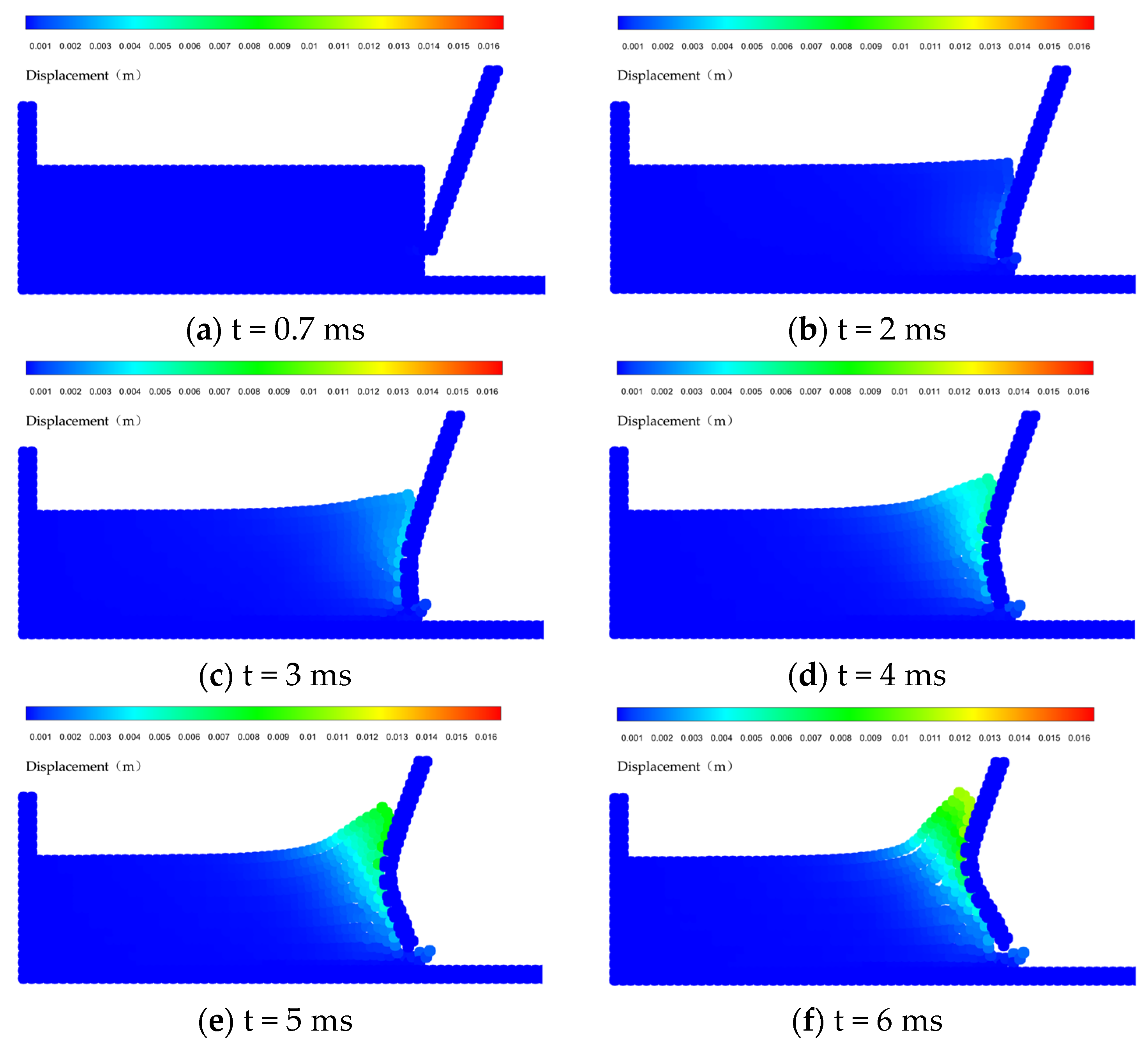
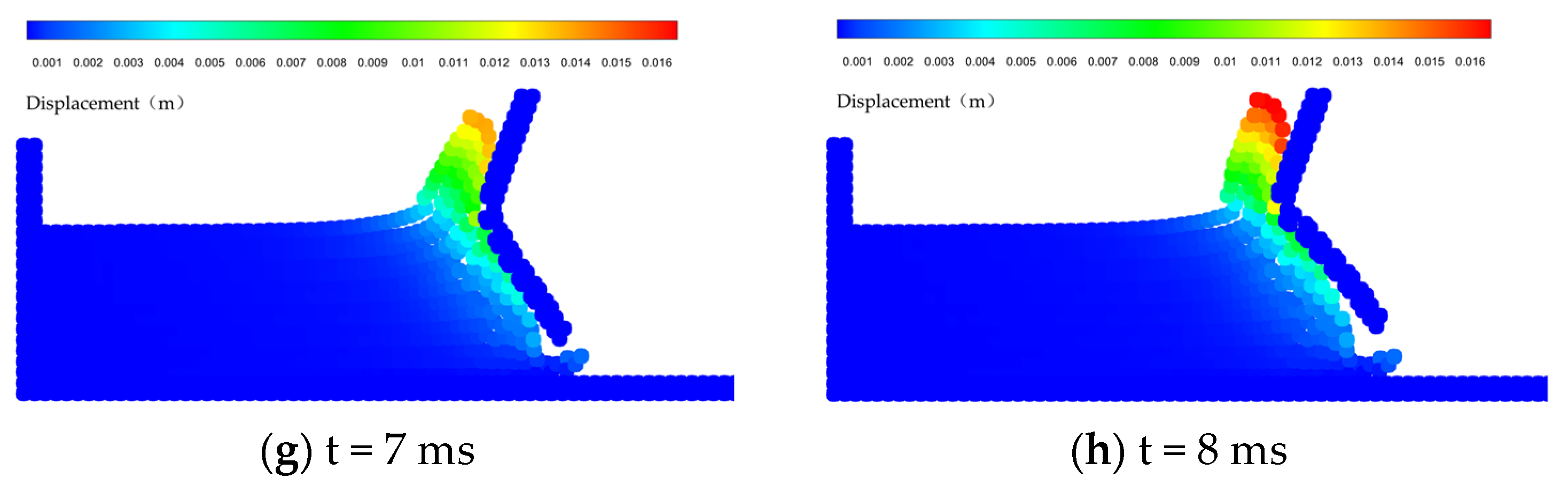
3.3. Distribution of Soil Displacement

The dynamic cutting motion of agricultural tillage tools induces complex extrusion and shear deformations in the soil, and shear deformations tend to occur at locations where the cumulative plastic strain is large. As shown in Figure 7, the formation of soil shear zones can be predicted by observing the changes in cumulative plastic strain.
When the soil is disturbed, the discrete soil particles are displaced in a highly non-uniform manner, depending on their spatial location. As depicted in the particle visualizations in Figure 8, the soil particles directly along the cutting edge experience the most intense compressive and shearing forces as the leading edge of the tool actively drives the soil flow. In contrast, the soil particles located below and along the length of the tool undergo lower overall displacements.
This is particularly evident after a fracture occurs, where the fractured segment of the tool substantially disrupts the underlying soil movement, causing decreased soil displacements in the middle and lower portions. This differential motion reflects the soil deformation field generated by the complex progressive interactions with the deforming and fracturing tool. Thoroughly analyzing these heterogeneous soil displacements provides the opportunity to relate localized soil deformation behaviors to the performance and fracture failures of the specific tool geometries and operating conditions. These fundamental insights can then be leveraged to optimize the tool designs and tillage parameters to achieve more uniform displacement distributions throughout the soil, potentially improving tillage effectiveness and efficiency. For instance, modifying tool geometries and cutting angles to reduce fractures may assist in producing more consistent soil displacements. By enabling detailed analysis of the complex coupling effects and spatial variations, this study facilitates the enhanced design of agricultural tillage tools for improved performance, fracture resistance, and tillage effectiveness.

3.4. Velocity Vector Analysis

Analyzing the velocity variations of the tool and the soil helps to verify the above results for the tool deformation and soil displacement distribution. Figure 9 shows the velocity vector plots of the tool and soil, where the color and length of the arrow line segments represent the velocity magnitude of each particle, and the direction of the arrow represents the velocity direction of each particle. The figure directly visualizes the velocity state of tool particles and soil particles at different moments.
The results show that the trend of tool deformation and soil displacement distribution are consistent with the velocity of the tool particles and soil particles. After the tool contacted the soil, the velocity of the lower portion of the tool particles changed, and the larger the velocity variable, the larger the tool deformation; meanwhile, the deformation trend was consistent with the velocity direction. The greater the velocity of the soil particles along the above cutting edge, the greater the soil particle displacement; the location of the soil accumulation formation was also consistent with the velocity direction.

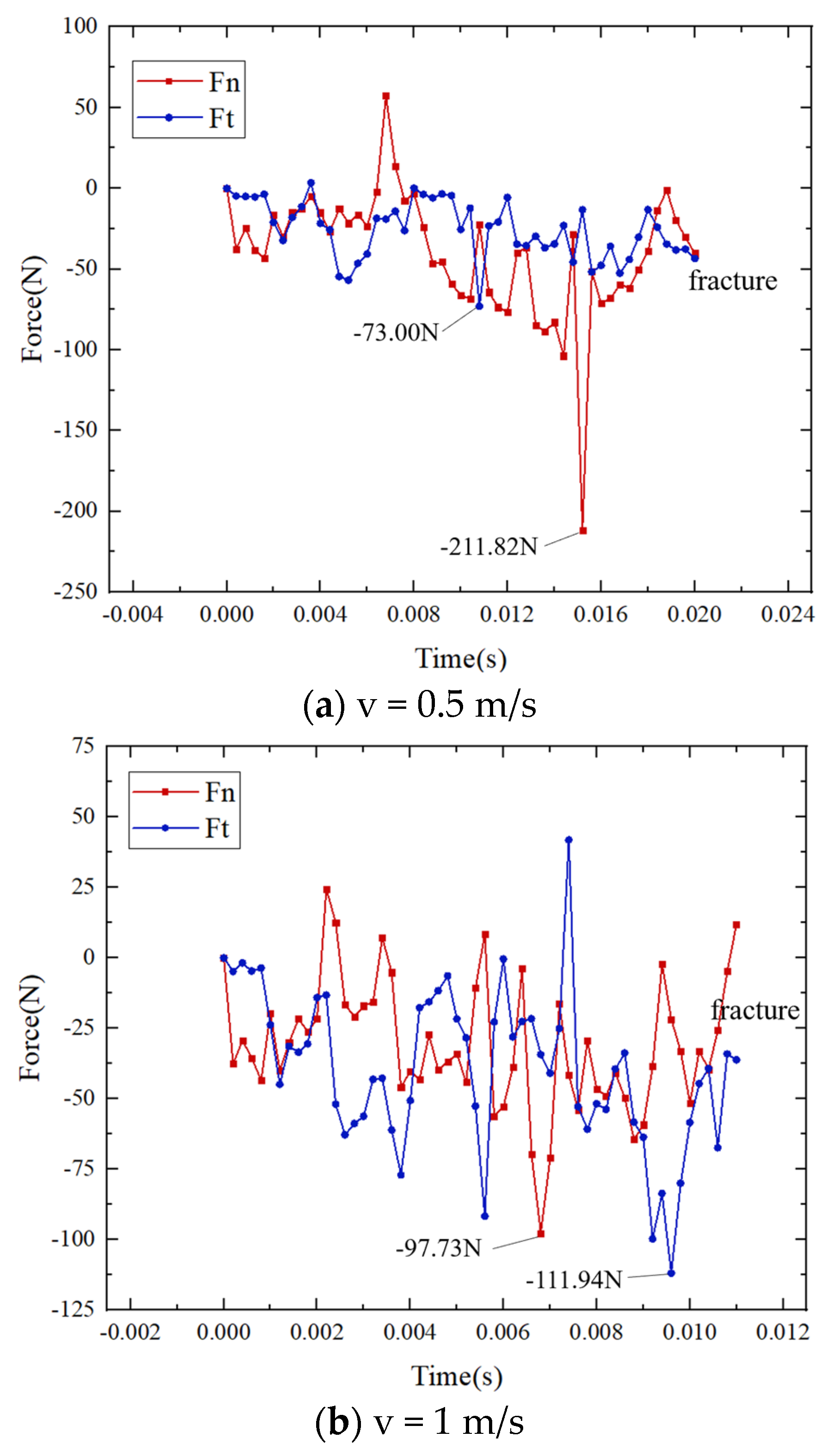
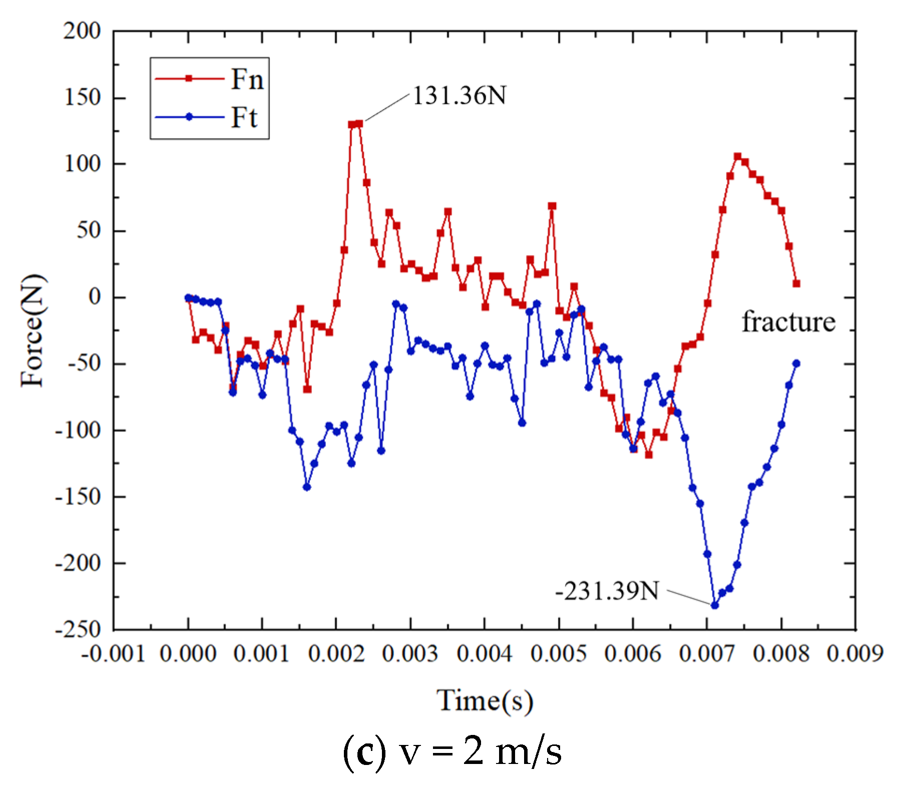
3.5. Cutting Force Analysis

Cutting force is an important parameter that directly governs energy consumption, efficiency, and reliability during agricultural tillage operations. Accurately modeling the evolution of the resulting cutting forces on the tool over time is therefore essential for optimizing the performance and durability of tillage tools. In this study, the evolution of the cutting forces on the tool is simulated over time by modeling the complex interactive forces between the dynamic tool and discrete soil particles. Figure 10 presents the detailed simulated profiles of both the normal and tangential cutting force components developing along the tool surface under three different tool cutting speeds: 0.5 m/s, 1 m/s, and 2 m/s, respectively. The cutting force magnitudes and durations are shown to vary quantitatively based on the different tool speeds, reflecting differences in soil deformation rates and tool damage progression. Tracking the force development throughout the cutting process at these representative speeds enables in-depth studies of the relationships between tool geometry, operating parameters, and resulting loads on the tool. This facilitates the enhanced design of agricultural tillage tools for optimal energy efficiency and prolonged service lifetimes under the harsh soil-cutting environment parameters.
As shown through the cutting force profile comparisons in Figure 10, the overall qualitative trends and force evolution stages are relatively consistent across the different tool speeds analyzed. However, the force magnitudes and durations vary quantitatively based on the distinct cutting velocities. Examining the representative case with a cutting speed of 2 m/s provides detailed insights for correlating the progressive cutting force development with the tool’s deformation and damage processes. Initially, at 0.7 ms after the tool contacts the soil, the cutting force rapidly increases as the resisting soil applies increasing loads on the advancing tool. This sharp rising force trend is attributed to the growing soil cutting resistance as the tool–soil interface expands laterally and soil builds up along the tool surface. Around 2 ms, the onset of substantial plastic deformation in the tool structure causes a slight drop and fluctuations in the cutting forces. In the subsequent plastic strengthening stage, the cutting forces gradually increase again as additional loads are applied over larger contact areas. The forces peak at 7 ms as tool fracture initiates, followed by a declining trend as loads are relieved by the fracturing tool. Tracking this intimately coupled force–deformation history highlights the direct relationships between cutting forces and accumulating damage in the tool.
Combined with the trends of cutting forces during the tool deformation process and the deformation of the tool in the above conclusions, it is found that these results coincide with the four stages of metal deformation (elastic, yield, strengthening, and necking stages), thereby proving the correctness of the coupled soil–tool model proposed in this paper.
This understanding of these tight correlations facilitates the optimization of agricultural tillage tool designs for enhanced fracture resistance and durability. For instance, modifying geometries to sustain cutting loads while reducing damage accumulation will improve tool performance and longevity over prolonged operation cycles. Overall, these simulations capturing the interactive cutting physics provide an effective platform for studying design enhancements that can meet the demanding mechanical requirements of soil tilling equipment and operations.

4. Conclusions

This study utilizes the SPH method to simulate the progressive plastic deformation and ductile fracture failure of agricultural tillage tools. The coupled soil–tool model calculates the complex interactions and predicts the damage process:
(1)
The model combines an elastoplastic constitutive model and the Johnson–Cook damage criterion, incorporating Lennard-Jones repulsive forces for the soil–tool interface coupling. Numerical techniques including the artificial stress terms and Jaumann rate correction handle the challenges of cohesive soil, stress fluctuations, and large deformations. This enables simulation of the complete progressive failure sequence from initial loading to final fracture.
(2)
Simulations reveal the detailed post-fracture displacement fields in the soil, highlighting the non-uniform distributions. Velocity vector plots visualize and accurately reflect the motion of the tool and soil particles. The coupled force–deformation tool response provides insights into the relationships between cutting forces and accumulating tool damage. This fundamental understanding facilitates the optimization of tool structural design for enhanced fracture resistance.
(3)
Overall, the model accurately characterizes the complex soil–tool interactions involving substantial stresses and deformations. This technique could be extended to simulate progressive damage in other earthmoving equipment components, providing a versatile simulation platform.

Author Contributions

Methodology, H.F. and M.H.; Software, T.G.; Formal analysis, H.F., Y.R. and M.H.; Investigation, S.Y.; Data curation, H.F., T.G. and M.H.; Writing—original draft, H.F.; Writing—review & editing, M.H.; Visualization, H.F., Y.R. and Q.T.; Supervision, A.B. All authors have read and agreed to the published version of the manuscript.

Funding

This research was funded by The Science and Technology Support Program Project of Guizhou Province, grant number [2021] General 341.

Data Availability Statement

The data presented in this study are available on request from the corresponding author.

Conflicts of Interest

Author Tao Gao was employed by the company Chongqing Chang’an Technology Co., Ltd. The remaining authors declare that the research was conducted in the absence of any commercial or financial relationships that could be construed as a potential conflict of interest.

Nomenclature

Ω problem domain
δ Dirac function
W smoothing kernel function
hsmooth length
V particle volume
mparticle mass
x coordinate position
vvelocity
einternal energy
σ α β stress tensor
α , β Cartesian components
Ppressure
ρ density
μ dynamic viscosity coefficient
Ntotal number of particles within the support domain
K i j artificial stress term
Π i j artificial viscosity term
ε ˙ α β strain rate tensor
ω ˙ α β rotation rate tensor
λ ˙ plastic multiplier
τ α β deviatoric shear stress
Γ 0 Gruneisen’s constant
S a linear Hugoniot slope coefficient
Gshear modulus
σ y yield stress
J 2 second stress tensor invariant
ε e f f p equivalent plastic strain
Δ ε e f f p increment of equivalent plastic strain
ε ˙ e f f p equivalent plastic strain rate
A, B, C, N, and MJ–C plasticity model constants
T * normalized temperature
T r e f reference temperature
T m e l t melting temperature
ε f a i l u r e failure strain
ccohesive force
Φ friction angle
Kbulk modulus
υ Poisson’s ratio
C p specific heat
Abbreviations
SPHsmoothed particle hydrodynamics
FEMfinite element method
DEMdiscrete element method
D-PDrucker–Prager yield criterion
J-CJohnson–Cook constitutive model

References

  1. Li, H.; Hao, J.; Zhao, J.; Ma, Y.; Li, J. The status and enlightenment of research on soil abrasion mechanism of soil—Engaging components of agricultural machinery abroad. J. Agric. Mech. Res. 2022, 44, 1–6. [Google Scholar] [CrossRef]
  2. Zhou, B.; Tian, G.; Shu, L.; Lan, X. Analysis on the weak points of the development of agricultural mechanization in Chongqing. Farm Mach. 2022, 65–68+71. [Google Scholar] [CrossRef]
  3. Su, B.; Xu, Y.; Jian, J. The actuality of development and research of wear resistant part for agricultural mechinery. Heat Treat. Technol. Equip. 2013, 34, 53–58. [Google Scholar] [CrossRef]
  4. Zhong, J.; Ren, S.; Wu, M. Numerical simulation of rotary tillage and soil cutting based on smooth particle hydrodynamics. J. Hunan Agric. Univ. (Nat. Sci.) 2022, 48, 744–748. [Google Scholar] [CrossRef]
  5. Wang, Y.; Wang, Z.; Ma, S.; Ge, J. Simulation of vertical trenching process based on SPH algorithm. Jiangsu Agric. Sci. 2018, 46, 225–228. [Google Scholar] [CrossRef]
  6. Lu, C.; He, J.; Li, H.; Wang, Q.; Zheng, Z.; Zhang, X. Simulation of soil cutting process by plane blade based on SPH method. Trans. Chin. Soc. Agric. Mach. 2014, 45, 134–139. [Google Scholar] [CrossRef]
  7. Gao, T.; Xie, S.; Hu, M.; Tan, Q.; Fang, H.; Yi, C.; Bao, A. Soil-soil engaging component SPH model based on a hypoplastic constitutive model. Trans. Chin. Soc. Agric. Mach. 2022, 38, 47–55. [Google Scholar] [CrossRef]
  8. Cao, Z.; Cui, J.; Zhan, X.; Li, Y.; Wang, Y.; Yu, X.; Liu, W.; Song, S. Simulation and experimental study of soil cutting process by subsoiler based on SPH method. J. Agric. Mech. Res. 2019, 41, 28–34+41. [Google Scholar] [CrossRef]
  9. Sun, H. Simulation and experimental study of soil cutting process by ditching component in orchard. J. Chin. Agric. Mech. 2019, 40, 190–194. [Google Scholar] [CrossRef]
  10. Liu, Y.; Wang, X.; Fen, M.; Zhang, H. The soil cutting dynamics simulation and research based on SPH /FEM coupling algorithm. J. Agric. Mech. Res. 2017, 39, 21–27+33. [Google Scholar] [CrossRef]
  11. Zhu, L.; Sun, Y.; Wang, H.; Leng, Z.; Yang, L.; Yang, M. Simulation of cutting soil of the mini-tiller rotary blade roller based on Finite Element Method. J. Agric. Mech. Res. 2020, 42, 39–43. [Google Scholar] [CrossRef]
  12. Han, Y.; Li, Y.; Zhao, H.; Chen, H.; Liu, D. Simulation of soil cutting by vertical rotary blade based on SPH method. J. Southwest Univ. (Nat. Sci.) 2016, 38, 150–155. [Google Scholar] [CrossRef]
  13. Zhu, C.; Zhu, L.; Huang, C. Simulation research of soil cutting based on FEM-SPH method. J. Agric. Mech. Res. 2015, 37, 54–58. [Google Scholar] [CrossRef]
  14. Yang, J.; Wang, C.; Wang, F.; Yang, X. Simulation of soil-tillage tool interaction using finite element analysis. J. China Agric. Univ. 2015, 20, 185–193. [Google Scholar] [CrossRef]
  15. Fang, H.; Ji, C.; Zhang, Q.; Guo, J. Force analysis of rotary blade based on distinct element method. Trans. Chin. Soc. Agric. Mach. 2016, 32, 54–59. [Google Scholar] [CrossRef]
  16. Zhang, X.; Zhang, L.; Shan, Y.; Wang, H.; Shi, X. Finite Element simulation research and key parameter optimization of rotary plowing parts. J. Agric. Mech. Res. 2023, 45, 36–42. [Google Scholar] [CrossRef]
  17. Zhang, Z.; Chen, Z.; Lai, Q.; Sun, W.; Xie, G.; Tong, J. Design and experiments of the Bouligand structure inspired bionic wear resistant soil-engaging component for the agricultural machinery. Trans. Chin. Soc. Agric. Mach. 2023, 39, 28–37. [Google Scholar] [CrossRef]
  18. Zhou, A.; Luo, H.; Xu, X.; Xu, Q.; Zhu, Y. Numerical simulation of soil cutting process based on material point method. Mech. Electr. Eng. Technol. 2023, 52, 1–6+171. [Google Scholar] [CrossRef]
  19. Niu, W.; Mo, R.; Sun, H.; Han, Z. Predication of the titanium alloy's chip morphology based on TANH constitutive model and smoothed particle hydrodynamic method. J. Shanghai Jiao Tong Univ. 2019, 53, 624–632. [Google Scholar] [CrossRef]
  20. Liu, G.R.; Liu, M.B. Smoothed Particle Hydrodynamics: A Meshfree Particle Method; World Scientific: Singapore, 2004. [Google Scholar]
  21. Zhou, X.; Ma, X.; Liao, X.; Qi, S.; Li, H. Numerical simulation of abrasive water jet impacting porous rock based on SPH method. Chin. J. Geotech. Eng. 2022, 44, 731–739. [Google Scholar] [CrossRef]
  22. Ma, X.; Mamtimin, G.; Yan, Y.; Jin, A. Simulation and forecast the process of droplet impacting on elastic solid. Comput. Simul. 2020, 37, 242–246+338. [Google Scholar]
  23. Bui, H.H.; Fukagawa, R.; Sako, K.; Ohno, S. Lagrangian meshfree particles method (SPH) for large deformation and failure flows of geomaterial using elastic-plastic soil constitutive model. Int. J. Numer. Anal. Methods Geomech. 2008, 32, 1537–1570. [Google Scholar] [CrossRef]
  24. Dong, X.W.; Liu, G.R.; Li, Z.L.; Zeng, W. A smoothed particle hydrodynamics (SPH) model for simulating surface erosion by impacts of foreign particles. Tribol. Int. 2016, 95, 267–278. [Google Scholar] [CrossRef]
  25. Wang, B.; Xu, H.; Zhang, L.; Zhang, H.; Wang, H. Progressive prognosis rupture prediction based on Johnson-Cook damage criterion based on principal component regression. China Acad. J. Electr. Publ. House 2023, 167–174. [Google Scholar] [CrossRef]
  26. Bui, H.H.; Sako, K.; Fukagawa, R.; Wells, J. SPH-Based Numerical Simulations for Large Deformation of Geomaterial Considering Soil-Structure Interaction. In Proceedings of the International Conference of International Association for Computer Methods & Advances in Geomechanics, Goa, India, 1–6 October 2008. [Google Scholar]
  27. Monaghan, J.J. Simulating Free Surface Flows with SPH. J. Comput. Phys. 1994, 110, 399–406. [Google Scholar] [CrossRef]
Figure 1. Soil and solid particles near the interface.
Processes 12 00086 g001
Figure 2. Flow of tillage tool deformation and fracture model based on SPH method.
Processes 12 00086 g002
Figure 3. Tillage cutting model.
Processes 12 00086 g003
Figure 4. Deformation process of tillage tools.
Processes 12 00086 g004
Figure 5. Deformation variation curve at the front tip of the tool.
Processes 12 00086 g005
Figure 6. Deformation of different materials.
Processes 12 00086 g006
Figure 7. Cumulative plastic strain in soil.
Processes 12 00086 g007
Figure 8. Displacement distribution of soil particles.
Processes 12 00086 g008aProcesses 12 00086 g008b
Figure 9. Velocity vector.
Processes 12 00086 g009
Figure 10. Cutting force variation curve.
Processes 12 00086 g010aProcesses 12 00086 g010b
Table 1. Material parameters.
Material TypeMaterial PropertiesSymbolValue
SoilDensity ρ 1540 kg/m3
Cohesive forcec5 kPa
Friction angle Φ 28°
Bulk modulusK1.5 MPa
Shear modulusG0.9 MPa
Tillage toolDensity ρ 0 2800 kg/m3
Shear modulusG26 GPa
Poisson’s ratio υ 0.33
Melting temperature T m e l t 925 K
Specific heat C p 875 J/(kg K)
J–C plasticity modelA324 MPa
B114 MPa
N0.002
C0.42
m1.34
Disclaimer/Publisher’s Note: The statements, opinions and data contained in all publications are solely those of the individual author(s) and contributor(s) and not of MDPI and/or the editor(s). MDPI and/or the editor(s) disclaim responsibility for any injury to people or property resulting from any ideas, methods, instructions or products referred to in the content.

