Abstract
In many flexible job shop scheduling problems, transportation scheduling problems are involved, increasing the difficulty in problem-solving. Here, a novel artificial Physarum polycephalum colony algorithm is proposed to help us address this problem. First, the flexible job shop scheduling problem with transportation constraints is modeled as a state transition diagram and a multi-objective function, where there are ten states in total for state transition, and the multi-objective function considers the makespan, average processing waiting time, and average transportation waiting time. Second, a novel artificial Physarum polycephalum colony algorithm is designed herein with two main operations: expansion and contraction. In the expansion operation, each mycelium can cross with any other mycelia and generate more offspring mycelia, of which each includes multiple pieces of parental information, so the population expands to more than twice its original size. In the contraction operation, a fast grouping section algorithm is designed to randomly group all mycelia according to the original population size, where each group selects the best fitness one to survive, but the other mycelia are absorbed to disappear, so the population size recovers to the original size. After multiple iterations, the proposed algorithm can find the optimal solution to the flexible job shop scheduling problem. Third, a series of computational experiments are conducted on several benchmark instances, and a selection of mainstream algorithms is employed for comparison. These experiments revealed that the proposed method outperformed many state-of-the-art algorithms and is very promising in helping us to solve these complex problems.
1. Introduction
At present, the flexible job shop scheduling (FJSS) problem with transportation constraints is gaining more and more attention [1,2], with it comprising many machines and vehicles, where a series of jobs have to be arranged and a series of transportation tasks have to be handled. This kind of system is very popular in modern industry and smart logistics systems [3]. Until now, all kinds of vehicles, especially automated guided vehicles (AGVs) [4] and mobile robots (MRs) [5], have been widely applied to support flexible job shop scheduling systems and are integrated with them. Such vehicles can help transport raw materials or products from a dock to a storage facility or help transport all kinds of materials between different areas in a warehouse or on the production line [6]. In this environment, jobs are kept for transporting between different areas to be handled until all transportations are finished. Due to the deep involvement of vehicles, the flexible job shop scheduling problem with transportation constraints has become increasingly important.
In a flexible job shop scheduling problem with transportation constraints, there are two subproblems, namely, the job shop scheduling problem (JSSP) and the transportation scheduling problem (TSP) [7]. These two problems are interrelated and inseparable, and in studying one of them in isolation, one cannot obtain the optimal solution to the entire problem [8]. Some scholars choose to divide this complex problem into two simpler subproblems to solve them separately, thereby reducing the difficulty of solving the problem. For example, the job shop scheduling task is solved first without transportation constraints, and then, the vehicle transportation tasks are sequentially addressed [9]. However, this also leads to the loss of reference value in the solution results since a separate solution to this problem involves two kinds of scheduling operations where the separated scheduling tasks are closely interrelated.
The flexible job shop scheduling problem with transportation constraints is NP-hard since its two subproblems are NP-hard, i.e., the job shop scheduling problem (JSSP) and the vehicle scheduling problem (VSP) [10]. The latter is also called a transportation scheduling problem or a load/unload problem. Many researchers have proposed all kinds of artificial intelligence algorithms to solve these kinds of complex problems, i.e., genetic algorithms (GAs) [2,4], particle swarm optimization (PSO) [6], simulated annealing (SA) [6], ant colony optimization (ACO) [8], fuzzy logic (FL) [11], deep learning (DL), artificial neural networks (ANNs) [12], artificial bee colony (ABC) [13], and adaptive memetic algorithms (AMAs) [14]. The experimental results of these studies revealed that these artificial intelligence algorithms can obtain satisfactory results in job shop scheduling problems. In recent years, a unicellular organism has given us great inspiration, Physarum polycephalum [15]. It can generate thousands of mycelia to search for food and shrink into the most refined mycelium structure after finding food. Therefore, we attempted to design an artificial Physarum polycephalum colony algorithm to help us solve the FJSS problem.
The main contributions of this work are as follows:
First, the flexible job shop scheduling problem with transportation constraints is modeled as a state transition diagram and a multi-objective function, where there are ten states in total for state transition, and the job shop scheduling problem and transportation scheduling problem are integrated by mixed integer linear programming. The main objectives consider the minimization of the makespan, the minimization of the average processing waiting time, and the minimization of the average transportation waiting time. The objective function integrates the job scheduling performance and transportation scheduling performance. The constraints provide restrictive conditions among the scheduling jobs, machines, and vehicles and ensure that the products are efficiently transported to the final users.
Second, based on the swarm intelligence of natural Physarum polycephalum, a novel artificial Physarum polycephalum colony (APPC) is designed to help us solve this kind of complex flexible job shop scheduling problem with transportation constraints. Our proposed algorithm utilizes two main operations: expansion and contraction. In the expansion operation, each mycelium can cross with any other mycelia and generate more offspring, with each one including multiple parental information, so the population expands to more than twice its original size. In the contraction operation, a fast grouping section algorithm is designed to randomly group all mycelia according to the original population size, where each group selects the best fitness one to survive, but the other mycelia are absorbed to disappear, so the population size recovers to the original size. Therefore, the expansion operation increases the global search ability, and the contraction operation increases the quick convergence ability. After multiple iterations, the proposed algorithm can find the optimal solution to the flexible job shop scheduling problem.
Third, a series of numerical examples are tested, and some mainstream artificial intelligence methods are compared. The proposed APPC algorithm is good at searching for optimal solutions and outperforms many state-of-the-art algorithms in terms of time performance and space performance.
The remainder of this paper is organized as follows: Section 2 presents a brief literature review of the research progress on the FJSS problem; Section 3 illustrates the mathematical model of the flexible job shop scheduling problem with transportation constraints; in Section 4, a novel APPC algorithm is explored; in Section 5, a series of computational experiments are implemented to test the proposed APPC algorithm and compare it to other algorithms; and finally, in Section 6, some interesting conclusions are drawn and future research directions are presented.
2. Literature Review
Traditional job shop scheduling problems often neglect the travel times or assume that unlimited transport resources are available. These cases are often inconsistent with engineering practice because vehicle transportation tasks are very common in the FJSS problem. If the vehicle transportation problem cannot be fully considered, the optimal solution to the job scheduling problem will not be obtained. The job shop scheduling problem with transportation constraints needs to decide the machine scheduling, vehicle scheduling, and transportation assignment. Ref. [2] designed a multistart biased random key genetic algorithm for the flexible job shop scheduling problem with transportation. Solving these interrelated problems is helpful in improving the operational performance of the job scheduling system. Refs. [4,16] proposed an integrated scheduling method of machines and automated guided vehicles in a flexible job shop environment based on genetic algorithms.
The use of mobile robots also brings transportation issues. The authors of [5] modeled the job shop scheduling problem as a mixed integer linear programming (MILP) model and considered the routing problem of mobile robots. A mixture of job shop scheduling systems and transportation scheduling systems also increases the factors considered during scheduling. Ref. [7] produced a job shop scheduling joint consideration of production, transport, and storage/retrieval systems. Ref. [9] addressed the energy-efficient job shop scheduling problem with transport resources, considering speed-adjustable resources. These works revealed that the benefits of integrating job shop scheduling and transportation scheduling can greatly improve the job completion time and operational performance.
Many research works often independently study job shop scheduling problems and vehicle transportation problems, such as dynamic job shop scheduling [12,17], interval job shop [13], energy-efficient distributed flexible job shop scheduling [14], limited waiting time constraint on a hybrid flowshop [18], embedded environment [19], and flexible job shop scheduling [20]. Ref. [21] presented a dynamic configuration method of flexible workshop resources based on an imperialist competitive algorithm hybrid neighborhood search (IICA-NS). Although doing so can reduce the difficulty of solving a problem, it leads to a lack of coordination since sub-optimal solutions and cannot reach global optimization. Recent research progress indicates that neglecting transportation scheduling in job shop scheduling may result in serious consequences [22], such as low resource utilization, unexpected bottlenecks, high intermediate inventories and operational costs, and low user satisfaction.
The integration of job shop scheduling and vehicle scheduling makes the scheduling problem more challenging since the multi-objective decisions and constraints become more complex [17]. Ref. [23] employed a multi-agent system simulation-based approach for collision avoidance in an integrated job shop scheduling problem with transportation tasks. Many researchers have demonstrated that there are a lot of conflicting factors in coordinating job shop scheduling and transportation scheduling. For example, ref. [24] introduced an approach to the integrated scheduling of flexible job shop scheduling, considering conflict-free routing problems. In engineering practice, a flexible job shop scheduling task often transports materials from one workstation to another or from a load/unload area to another, which are inevitably involved in vehicle transportation scheduling [25].
Now, current mainstream scientists consider this kind of FJSS problem to be multi-objective with many conflicting factors and NP-hard, so traditional, exact approaches can only be applied to solve small-sized cases [1]. It is very important and challenging to design efficient algorithms to address it in large-sized cases, such as simulated annealing (SA) [6] and fuzzy logic (FL) [11]. Among them, swarm intelligence (SI) algorithms have received great attention [23,26], i.e., genetic algorithms (GAs) [2,4,16], particle swarm optimization (PSO) [6,19], ant colony optimization (ACO) [8], deep learning (DL), artificial neural networks (ANNs) [12,27], artificial bee colony (ABC) [13], adaptive memetic algorithms (AMAs) [14], migrating birds optimization [17], grey wolf optimization (GWO) [20], quantum cat swarm optimization [22], artificial slime mold [28], artificial Physarum swarm [29], coronavirus herd immunity [30], artificial plant community [31,32], whale optimization [33], artificial algae [34], and the Jaya algorithm [35]. However, these swarm intelligence algorithms are also prone to fall into local optimization prematurely, and some scholars have tried to improve algorithm performance using hybrid algorithms [6,36].
In recent years, a unique creature has given us new inspiration. Natural Physarum polycephalum can generate countless mycelia for expansion and then shrink into the optimal network structure after finding food [15]. Some researchers have tried to simulate their search behavior [28,29], but the current research works have not fully explored the core functions of the Physarum polycephalum colony, i.e., swarm learning, expanding the population size to increase the search ability, and shrinking the population size to optimize solution results.
The following research gaps currently exist:
- Traditional artificial intelligence algorithms and swarm intelligence algorithms both use a fixed population size, while the population size of Physarum polycephalum varies significantly during expansion and contraction, and the increased population size also enhances its global search ability.
- Traditional artificial intelligence and swarm intelligence algorithms typically use pairwise learning, where two individuals learn from each other to produce a pair of new individuals. The Physarum polycephalum allows each mycelium to cross with multiple other mycelia to produce offspring containing information from a lot of parents.
- Traditional artificial intelligence and swarm intelligence modify the values of all individuals in each iteration, making it easy to lose the optimal solution. However, the Physarum polycephalum allows for the preservation of the optimal solution for each iteration.
If we can design an efficient algorithm based on its search behavior, it may help us solve many difficult problems. This is the motivation for this research work.
3. Problem Modeling
Based on the benchmark tests in [37,38], this section describes the flexible job shop scheduling problem with transportation constraints, including a state transition diagram, a multi-objective function, and constraints.
In a flexible job shop scheduling problem with transportation constraints, the main components are composed of a production system and a transportation system. The production system comprises a series of machines and a series of independent jobs, where every job contains a series of ordered operations and has its own independent machine order. Any ordered operation must be handled on a committed machine in a predefined processing period without interruption. At the same time, every machine can only handle one operation at a time, and every job can only be processed on one machine at a time. Hence, this part is a classic job shop scheduling problem.
The transportation system incorporates a number of identical vehicles with the same speed and load capacity, which can execute any transportation task. In a flexible job shop scheduling problem, every vehicle can only carry one job at a time. It is often assumed that the layout and the travel times between any two nodes are predetermined, and transportation scheduling is non-preemptive. To simplify the analysis, carpooling [39] and platooning [40] are not considered here.
3.1. Symbol Definitions
This section provides the symbol definitions used in the next sections, as shown in Table 1.

Table 1.
Symbol definitions.
For a flexible job shop scheduling problem with transportation constraints, there is a job set J with, at most, jmax of jobs, a machine set M with, at most, mmax of machines, and a vehicle set V with, at most, vmax of vehicles. In each job j, there is an operation set {Oj}, where the maximum number of jobs j is Ojmax. Each operation can be assigned to any machine for operation or any vehicle for transportation. There are two binary variables for machine assignment and vehicle assignment in job shop scheduling, i.e., AMm(Oji) and AVv(Oji). The binary variable of machine assignment AMm(Oji) indicates that the machine m is assigned to the operation Oji of the job j. The binary variable of vehicle assignment AVv(Oji) indicates that the vehicle v is assigned to the operation Oji of the job j.
For the flexible job shop problem, the integer programming method is used to define a feasible solution variable x. In each iterative computation, the APPC will use a multi-objective function to search for the optimal solutions, and the iteration counter Ite is used to count the iterative computation of the APPC. The self-learning is fixed, and the social-learning possibility ps and free-learning possibility pf are probabilistic to instruct the swarm searching process. If the solution error e reaches the error threshold eth, or the iteration counter Ite amounts to the maximum value Ite_max, then the iterative computation can be terminated to output the optimal solution.
3.2. A State Transition Diagram
In a flexible job shop scheduling problem with transportation constraints, a transportation task requires a pair of loading and unloading operations. The load operation requires an empty vehicle for transportation, and the unload operation requires an empty unloading area waiting for the vehicle to arrive. To illustrate this complex scheduling problem, we have designed a state transition diagram for FJSS jobs, as shown in Figure 1. There are ten states in total for each job, corresponding to the ten ellipses in the figure. In addition, the arrows between the ellipses indicate the direction of the state transition, and the text on the arrows indicates the machine or vehicle action that corresponds to the state transition. The ten states are illustrated as follows:
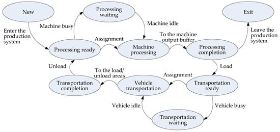
Figure 1.
The state transition diagram of the flexible job shop scheduling problem with transportation constraints.
- New: This is the first state. If a job enters a production system, it should be created first, where all machines are not occupied and each vehicle is located in the load/unload areas from the beginning.
- Processing ready: This is the second state. After creation, if a job enters the production system, or every job is transported by a vehicle from the load/unload areas and unloaded to a production system, it is in a ready state. This means that a job is ready for the machine for the processing operation.
- Machine processing: Although the job is ready, the machine may not be ready. If a machine is idle, then the machine can be assigned and the machine processing operation starts immediately. During the machine processing operation, the machine cannot be used for other purposes.
- Processing waiting: If the job is ready, but the machine is busy, then the assignment cannot be made and the job waits in the input buffer. Processing waiting will not end until there are idle machines to be assigned, and the job will enter the machine for processing operation.
- Processing completion: Whenever a processing operation is completed, the job is transferred to the machine output buffer and waits for the arrival of a vehicle for loading. The machine is ready for the next processing operation.
- Transportation ready: If a job is already available for transportation, it is ready for loading by an assigned vehicle.
- Vehicle transportation: Although the job is ready, the vehicle may not be ready. If a vehicle is idle, then the vehicle can be assigned to the job. Then, the job is loaded by the vehicle and transportation starts immediately. During this transportation process, the vehicle cannot be used for other purposes.
- Transportation waiting: If the job is ready, but the vehicle is busy or late for the assignment, the transportation has to wait. Transportation waiting will not end until there are idle vehicles to be assigned, and the job will be loaded for transportation.
- Transportation completion: When the vehicle arrives at the load/unload areas for the next processing operation, the transportation task is completed, and then, the job is unloaded to a machine and becomes ready for processing.
- Exit: This is the last state. If all job processing operations have been completed and all transportation tasks have been finished, the job is returned to the load/unload areas to leave the production system.
The ten states must be strictly transitioned in the direction of the arrows. In the processing ready state, as soon as the vehicle reaches the machine, it unloads the job and waits for the next transportation assignment. At the same time, the job is ready for machine processing. Once a processing operation of a job is completed on a machine, an idle vehicle will be assigned to load the job from the machine and transport the job to another machine for the next processing operation.
In the first schedule, a job is created as a new state, and the vehicles are required to transport jobs from the load/unload area to the machine processing area. The first schedule is slightly different from the subsequent schedules, where the first job requires a vehicle to transport it into a load/unload area before entering the production system. In this case, a job with n operations needs n transportation tasks. To simplify the analysis, all vehicles are assumed to have stopped there from the beginning. However, the entanglement between job scheduling and transportation scheduling still makes problem modeling more difficult.
In subsequent schedules, other than the first one or the last one, in most cases, it only considers the job scheduling with transportation between machine operations, so a job with n operations needs n − 1 transportation tasks. The job shop scheduling starts with the machine processing operation and ends with the last machine operation, but each operation requires waiting for the transportation task to be completed before proceeding.
In the last schedule, there may be an additional transportation task and the job will be in the exit state. In this case, a job with n operations needs n transportation tasks. This may result in asynchronous and additional transport tasks if the last job needs to be transferred to the load/unload areas when all operations have been completed. To diminish asynchronous transport tasks, a nope operation with zero processing time can be defined to handle the job at the load/unload areas. A nope operation is a virtual operation that does not consume any machine or vehicle resources nor does it take up any time. When a job is returned to the load/unload areas, a nope operation can be added to help the job be transported to a determined machine or a load/unload area. The completion time of a job will not be affected by the nope operation before the job is returned to the load/unload areas.
3.3. A Multi-Objective Function
Here, a mixed integer linear programming model is introduced to build a multi-objective function for the job shop scheduling problem. The main objectives include the minimization of makespan, the processing waiting time, and the transportation waiting time. The three objectives consider the job performance of all processing operations on machines and the transportation performance on all vehicles. If any of the two waiting times are long, this means low scheduling efficiency and a great waste of time, where all processing operations and all transport tasks require more time to wait to return the jobs into or out of the load/unload areas. In this case, the performance of the production operation will be adversely affected.
Objective function = {min{SP}, min{WM}, min{WV}}
Subject to:
The objective function in Equation (1) is to minimize the makespan, average processing waiting time, and average transportation waiting time. The three objectives may be conflicted in many cases, so simply pursuing the minimization of a goal cannot guarantee the efficiency of the entire job shop scheduling.
The following equations after Equation (1) are constraints, and their values limit the minimization of the objective function.
Constraint 1 in Equation (2) indicates that the binary variable AMm(Oji) of the machine assignment and the binary variable AVv(Oji) of the vehicle assignment can only take values of 0 or 1.
Constraint 2 in Equation (3) indicates that the machine start time , processing time , and end time are all non-negative.
Constraint 3 in Equation (4) indicates that the vehicle start time , transportation time , and end time are all non-negative.
Constraint 4 in Equation (5) indicates that all scheduling machines at a time cannot exceed the total number mmax of machines.
Constraint 5 in Equation (6) indicates that all vehicles scheduled at once shall not exceed the total number vmax of vehicles.
Constraint 6 in Equation (7) indicates that the end time of the job processing should not be less than the required machine processing time, the required vehicle transportation time, or the last machine end time of the previous job or operation.
Constraint 7 in Equation (8) indicates that the end time of the job transportation on different machines should not be less than the last machine processing time or required transportation time.
Constraint 8 in Equation (9) indicates that the start time of the machine m cannot be earlier than the previous end time or .
Constraint 9 in Equation (10) indicates that on a machine m, different operations are processed in a first-come-first-served way to ensure that the operations arriving first can be processed immediately.
Constraint 10 in Equation (11) indicates that on different machines, different operations of the same job j should be carried out in order to ensure that the operations are processed immediately upon arrival.
Constraint 11 in Equation (12) indicates that on a vehicle v, different jobs are assigned in a first-come-first-served way to ensure that the jobs that arrive first can be transported immediately.
Constraint 12 in Equation (13) indicates that on different vehicles, different operations for the same job j or different jobs for the same operation should be carried out in a sequential manner to ensure that they are transported immediately upon arrival.
Constraint 13 in Equation (14) indicates the immediate start of the first operation of the first job.
Constraint 14 in Equation (15) indicates that the last job ends immediately.
3.4. Resolution Approach
In this section, the resolution for the multi-objective function in the previous section is illustrated. The resolution is to search for the optimal binary variable of the machine assignment and the binary variable of the vehicle assignment and generate the optimal objective function in Equation (1).
As for the makespan, there are two cases. In Case 1, if the job at first starts from the load/unload area and directly enters into the production system, no vehicle transportation is required before entering the production system, and the job is completed after the last transportation. Then, the makespan can be calculated as
Equation (16) states that the makespan of all operations depends on the difference between the latest vehicle transportation end time and the earliest machine start time .
In Case 2, if the job at first starts from a vehicle transportation before entering the production system, and the job completes after the last transportation, then the makespan can be calculated as
Equation (17) states that the makespan of all operations depends on the difference between the latest vehicle transportation end time and the earliest vehicle transportation start time .
For the average processing waiting time, WM is decided by the total number of machines, and the difference between the required processing time and the actual processing time of an operation on each machine. The earliest start time of all operations on the machine m can be calculated as follows:
The last end time of all operations on the machine m can be calculated as follows:
The actual processing time of an operation Oji on the machine m equals the difference between the machine start time and the machine end time . That is:
The actual transportation time of an operation Oji on the vehicle v equals the difference between the vehicle start time and the vehicle end time . That is:
Hence, the total actual processing time of all operations on the machine m can be calculated as follows:
Notice the actual processing time of an operation Oji on the machine m is not the required processing time Pji of operation Oji. The difference between them is the processing waiting time, so the average processing waiting time WM can be obtained through:
Similarly, the average transportation waiting time WV is decided by the total number of vehicles and the difference between the required transportation time and the actual transportation time of an operation on each vehicle. The earliest start time of all operations on the vehicle v can be calculated as follows:
The last end time of all operations on the vehicle v can be calculated as follows:
The total actual transportation time of all operations on the vehicle v can be calculated as follows:
Notice the actual transportation time of an operation Oji on the vehicle v is not the required transportation time Tji of operation Oji. The difference between them is the transportation waiting time, so the average transportation waiting time WV can be given by:
Based on the makespan in Equations (16) or (17), the average processing waiting time WM in Equation (23), and the average transportation waiting time WV in Equation (27), the optimal binary variable of the machine assignment and the binary variable of the vehicle assignment can be searched for the optimal solutions to the job shop problem.
As we can see from Equations (1)–(27), there are a lot of constraints for machines and vehicles, so the multi-objective function of the FJSS problem with transportation constraints is more complex than the traditional job shop problem. In the next section, a novel APPC algorithm is proposed to help us solve this problem.
4. An APPC Algorithm for FJSS
Drawing on the advantages and disadvantages of traditional swarm intelligence algorithms and considering the unique behavioral characteristics of a natural Physarum polycephalum colony, an APPC algorithm was explored to simulate the novel swarm intelligence. The proposed artificial Physarum polycephalum colony can use a lot of mycelia to expand and contract to search for the optimal solution to FJSS problem in Equations (1)–(15), that is, its population size is variable.
4.1. Artificial Physarum Polycephalum Colony
Ref. [15] surveyed the learning mechanism in the single-cell organism Physarum polycephalum. A natural Physarum polycephalum is a fan-shaped structure composed of numerous mycelia, as shown in Figure 2, where it can generate thousands of mycelia through expansion operations to search for external food or establish the most efficient path for digesting food through contraction operations. Multiple Physarum polycephalum constitute a colony, and different Physarum polycephalum can use a lot of mycelia to cross each other to exchange information, improving the efficiency of expansion and contraction. More mycelia in expansion can enhance its global searching and local searching, and the population size increases. Fast selection in contraction improves its local fast convergence ability, and the population size decreases. Different from a natural Physarum polycephalum colony, the proposed artificial Physarum polycephalum colony can only run on a personal computer. The whole APPC algorithm includes three main components, i.e., an artificial Physarum polycephalum colony, food sources, and a fitness function.
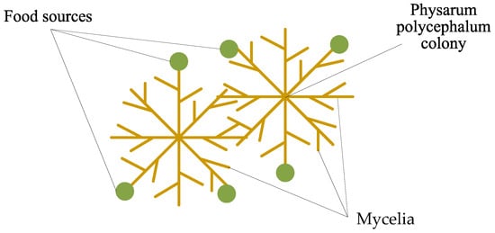
Figure 2.
The main architecture of the artificial Physarum polycephalum colony [15].
First, an artificial Physarum polycephalum colony is a swarm of APPC mycelia, and each mycelium can be encoded as a feasible solution to the FJSS problem. The traditional swarm intelligence algorithms often use a fixed population size, but the population size of the proposed APPC is variable. Its swarm learning mechanism contains self-learning, social learning, and free learning. All Physarum polycephalum mycelia can produce new mycelia or absorb other mycelia. Hence, its population size increases in expansion and decreases in contraction operations. This special swarm learning mechanism ensures that the APPC has a strong global search ability and local fast convergence ability.
Second, the food sources constitute a virtual solution space for an artificial Physarum polycephalum colony to live in. They are randomly distributed in the solution space, and the artificial Physarum polycephalum colony can search for food sources as feasible solutions to the FJSS problem. An artificial Physarum polycephalum mycelia connecting the food sources with high fitness will survive, otherwise, it will be absorbed or merged. An artificial Physarum polycephalum colony can search for the optimal solutions to share external food sources.
Third, a fitness function was used to evaluate the fitness of the artificial Physarum polycephalum colony, i.e., the FJSS model in Equations (1)–(15). The artificial Physarum polycephalum colony uses a lot of mycelia to expand and contract and tries its best to search for the optimal solutions. If an artificial Physarum polycephalum mycelium has a high fitness, it can be seen as a feasible solution.
Based on the above three components, the artificial Physarum polycephalum colony has two basic operations, i.e., expansion and contraction.
The expansion operation is the process of increasing the population size. The APPC utilizes three kinds of learning mechanisms to expand, i.e., self-learning, social learning, and free learning. Hence, there are three corresponding parts of mycelia after expansion, i.e., self-learning, social-learning, and free-learning mycelia. In the initialization, the artificial Physarum polycephalum colony obtains an original population size of S, where all mycelia are randomly encoded solutions. In the successive expansion operation, the self-learning mycelia keep a population size of S inherited from the previous iteration. Then, two new parts of mycelia are generated. The self-learning mycelia can cross with any other mycelia and generate a population size S of social-learning offspring mycelia, of which each includes a lot of parental information. However, another new part of free-learning mycelia is randomly produced by a free-learning possibility. Hence, the population size of the APPC after the expansion operation is twice greater than the original value S. This is helpful to improve the global searching capability.
The contraction operation is a process of decreasing the population size. The APPC will use a fast grouping section algorithm to randomly group all the mycelia according to the original population size S, where each group selects the best fitness one to survive, but the other mycelia are absorbed to disappear, so the population size recovers to the original size S. The multi-objective function is used to evaluate the fitness of the mycelia and instruct the APPC to select the best mycelium. The APPC will absorb a lot of mycelia with low fitness, and many mycelia will disappear after the contraction operation. The selection strategy can help preserve the best mycelia in iterative computing and improve the local convergence ability. With the repeated use of the expansion and contraction operations, the APPC can find the optimal solutions to the FJSS problem.
4.2. Algorithm Flow of the APPC
This section shows the algorithm flow of the APPC to the FJSS problem, as shown in Figure 3. The whole algorithm flow includes four main stages, namely initialization, expansion, contraction, and end judgment.
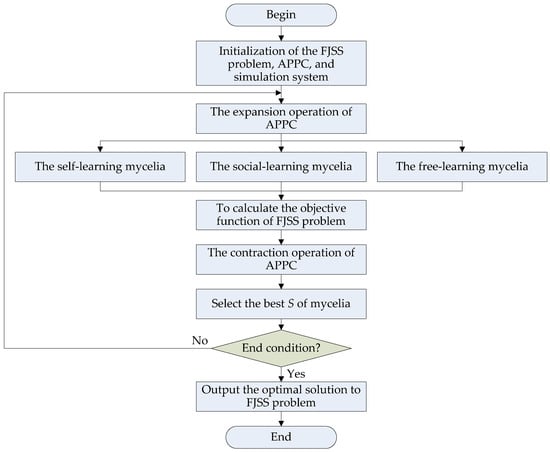
Figure 3.
The algorithm flow of the APPC for the FJSS.
In the initialization stage, there are three main parts, i.e., the FJSS problem, the APPC, and the simulation system. The initialization of the FJSS problem defines the jobs, machines, vehicles, and the multi-objective function in Equations (1)–(15). The initialization produces the initial mycelia of the APPC, and some important simulation parameters are also defined here.
In the expansion stage, the APPC will produce more mycelia to search for the optimal solutions to the FJSS. The self-learning, social learning, and free learning are implemented here, so the population size increases after expansion. The expansion process is a parallel search algorithm where three learning mechanisms are parallel and do not interfere with each other. The priority of these three learning processes does not affect the final solution, so there is no compulsory rule about choosing a direction or priority.
In the contraction stage, the APPC will evaluate the fitness of the mycelia and select the best S of the mycelia for the next iterative computation. The mycelia with low fitness are absorbed and disappear, so the population size decreases to the original value S.
The end judgment determines whether to continue or terminate the iterative computation. After many iterations of expansion and contraction, a predefined error threshold eth or the maximum of iterations Ite_max is employed for end justification before the optimal solutions to the FJSS problem are output.
The algorithm flow simulates the swarm intelligence of a natural Physarum polycephalum colony well and reveals its special search mechanism. Based on the algorithm flow in Figure 3, the following sub-sections further illustrate how to use the APPC to solve the FJSS problem and discuss the algorithm steps of our APPC algorithm, i.e., initialization, expansion, contraction, and end judgment. Then, it is helpful to observe that there is a great difference between our algorithm and traditional swarm ones.
4.3. Step 1: Initialization
The first initialization stage is to set the main parameters and the objective function to be solved, including the three main parts, i.e., the FJSS problem, the artificial Physarum polycephalum colony, and the simulation system.
First, the initialization of the FJSS problem includes setting the parameters of the jobs, operations, machines, and vehicles. There are three parts of the initialization parameters for the FJSS problem, i.e., a job set J with, at most, jmax of jobs, a machine set M with, at most, mmax of machines, and a vehicle set V with, at most, vmax of vehicles. In each job j, it is necessary to initialize the parameters of the operation set {Oj}, where the maximum operation number of job j is Ojmax, and each operation can be assigned in any machine for operation or any vehicle for transportation. There are two binary variables for machine assignment and vehicle assignment in job shop scheduling, i.e., AMm(Oji) and AVv(Oji). The binary variable of machine assignment AMm(Oji) indicates that the machine m is assigned to the operation Oji of the job j. The binary variable of vehicle assignment AVv(Oji) indicates that the vehicle v is assigned to the operation Oji of the job j.
Second, the initialization of the APPC is to set the main parameters related to the artificial Physarum polycephalum colony, including the population size S, the social-learning possibility ps, and the free-learning possibility pf. Each artificial APPC mycelium can be randomly initialized as a binary string x for AMm(Oji) and AVv(Oji), and the corresponding fitness can be initialized as zero. The multi-objective function in Equations (1)–(15) can be employed to evaluate the fitness. As a swarm intelligence algorithm, the initial values of {x} and their initial fitness values have nothing to do with the FJSS problem solving, and the APPC will ultimately find the optimal solution to the problem through repeated iterations.
Third, the initialization of the simulation system is required to provide a simulation environment. An iteration counter Ite should be defined and preset as zero. All the objective values in Equations (1)–(15) and the corresponding error e are initialized and cleared to zero. The end judgment for the iterative computation is initialized, i.e., the maximum iterations Ite_max, and the iteration error threshold eth. These parameters will determine whether the iterative calculation of the APPC ends or continues. This part of initialization determines when the simulation system starts and ends.
4.4. Step 2: Expansion
The expansion operation is the second stage of the APPC, where the population of the APPC expands and more mycelia are generated for swarm search. In the expansion operation, each mycelium can cross with any other mycelia and generate more offspring mycelia, which each include multiple pieces of parental information, so the population expands to more than twice its original size. The expanded mycelia {x} contain three parts, i.e., the self-learning mycelia {xself}, the social-learning mycelia {xsocial}, and the free-learning mycelia {xfree}.
First, the self-learning mycelia {xself(Ite)} completely inherit the solution from the previous calculation. It may be the initialization mycelia in the first iteration, or the optimal mycelia produced in the previous contraction stage. Note that this part of the mycelia is different between the first iteration and subsequent iterations. This part of the self-learning mycelia in the first iteration is random with corresponding random fitness values, so the optimal solution cannot be determined. The self-learning mycelia in the subsequent iterations are inherited from the optimal solutions in the previous contraction stages, so they have the optimal fitness in the last iteration.
Second, the social-learning mycelia {xsocial(Ite)} is generated by the self-learning mycelia {xself(Ite)} with the same population size S. It simulates the swarm learning of the natural Physarum polycephalum colony and each parent mycelium can exchange a piece of information with others to generate offspring mycelia. The social-learning mechanism is determined by a social-learning possibility ps, where division and cooperation will help the mycelia to expand the search space. Since the natural Physarum polycephalum colony undergoes single-cell asexual reproduction, it does not require pairing. Social learning can occur with any mycelia, and the possibility ps decides the ratio of information exchanging. The part of ps comes from a main parent mycelium and another part of 1-ps comes from any other parent mycelia, so each offspring mycelium includes multiple pieces of parental information. The larger the ps, the more experience comes from self-learning. On the contrary, the smaller the ps, the more experience comes from social learning. This helps improve the algorithm’s local convergence ability.
Third, the free-learning mycelia {xfree(Ite)} are randomly produced and are new solutions completely unrelated to the parent generation. The free-learning mycelia {xfree(Ite)} have nothing to do with the self-learning mycelia {xself(Ite)} and the social-learning mycelia {xsocial(Ite)}. Hence, the free-learning mycelia increase the global search capability. The population size is determined by the possibility pf, that is, the population size is S × pf. The smaller the pf, the more information comes from self-learning and social learning, the stronger the local convergence ability, and the faster its convergence speed. On the contrary, the larger the pf, the less information comes from self-learning and social learning, and the stronger the global search ability but the slower the convergence speed.
According to the self-learning population size of S, the social-learning population size of S, and the free-learning population size of Spf, the total population size increases to (2 + pf)S after expansion. The expansion operation endows the APPC algorithm with strong global search capabilities and strong local search capabilities. It can help the APPC algorithm solve the complex FJSS problem.
Here, the pseudo code of the expansion operation is presented here, as shown in Algorithm 1, where the top line is the title, and line 14 is Algorithm 2. It can be seen that the expansion operation has two cycles, so the time and spatial performance are linearly correlated with the maximum iterations and the population size of the APPC. Since the problem parameters are embedded in the APPC mycelia, such as the job set, operation set, machine set, and vehicle set, the problem scale has nothing to do with the solving performance. This can provide the APPC algorithm with good computational performance, which will not deteriorate sharply when the scale of the FJSS problem increases.
| Algorithm 1: Expansion operation |
| 1: Input: the FJSS problem, job set J = {Oji}, machine set M, vehicle set V 2: Input: APPC parameters, S, ps, pf 3: Define: fitness function in Equations (1)–(15) 4: Input: Ite_max, eth 5: Initialization: random mycelia {x} = {AMm(Oji), AVv(Oji)} 6: For iteration counter Ite = 1 to Ite_max 7: For APPC mycelia s = 1 to S 8: Self learning of {xself(Ite)} = {x(Ite − 1)} 9: Social-learning of {xsocial(Ite)} by ps 10: Free-learning of {xfree(Ite)} by pf 11: End for 12: To update the APPC mycelia {x} = {xself(Ite), xsocial(Ite), xfree(Ite)} 13: To calculate the fitness according to Equations (1)–(15) 14: // Algorithm 2: Contraction operation 15: End for |
Due to the population size of the artificial Physarum polycephalum colony being S and the maximum iterations being Ite_max, the time performance of expansion can be obtained as O(S × Ite_max), and the space complexity is O(S). In the two cycles of expansion, the APPC uses the total number of mycelia S to search for the total number of jobs jmax, the total number of machines mmax, and the total number of vehicles vmax and obtains (2 + pf)S solutions to the FJSS problem. The APPC expansion algorithm can acquire good search capabilities and good computational efficiency as well.
4.5. Step 3: Contraction
Contraction is the third stage for selecting the best S of mycelia from the expanded colony. In the contraction operation, a fast grouping section algorithm is designed to randomly group all mycelia according to the original population size, where each group selects the best fitness one to survive, but the other mycelia are merged to disappear, so the population size recovers to the original size. The colony calculates the fitness according to the multi-objective function in Equations (1)–(15) and uses a fast grouping section algorithm to select the optimal solutions to the FJSS problem. In the contraction stage, only the mycelia with high fitness can survive, but most mycelia with low fitness will be absorbed to disappear. The population size of the APPC is (2 + pf)S before contraction, but then, it decreases to S. This simulates the swarm learning of a natural Physarum polycephalum colony well and enhances the local convergence performance.
Here, a pseudo-code of the contraction operation is shown in Algorithm 2, where the top line is the title, and the first line is Algorithm 1. Algorithm 2 is reduced into line 14 in Algorithm 1, and the two algorithms each constitute two sub-algorithms of a complete APPC algorithm. An expansion operation and a contraction operation constitute a complete cycle. Here, a fast grouping section algorithm is employed to randomly divide the entire population into S groups, where it chooses the best mycelium for each group. Therefore, (2 + pf) mycelia can be randomly selected into a group, so a total of S optimal individuals will be selected from all groups, but the remaining individuals will be discarded or absorbed and disappear. Since the number of mycelia in each group can only be integers, the number of group members can be or , where int() is an integer operator, and the decimals after the decimal point will be directly discarded regardless of their values. Due to , the number of group members can be two or three.
The optimal solutions in each iterative computation can be selected from all S of mycelia:
The calculation error is calculated as follows:
| Algorithm 2: Contraction operation |
| 1: // Algorithm 1: Expansion operation 2: For APPC mycelia s = 1 to S 3: To randomly divide the APPC into S groups 4: To compare the fitness by Equations (1)–(15) 5: To choose the best mycelia from each group, each group has 2 or 3 mycelia 6: To store the temporary optimal fitness fitness(x*(Ite)) = max{fitness(x(Ite))} 7: To store the temporary optimal solution x* 8: To calculate the iterative error e = |fitness(x*(Ite)) − fitness(x*(Ite − 1))| 9: if e > eth 10: select the best S of mycelia 11: return to expansion algorithm 12: Else 13: Exit 14: End for 15: // Ite_max 16: output the optimal solution x* 17: output the optimal fitness fitness(x*) |
In Algorithm 2, the contraction algorithm has two cycles and is embedded in the iteration cycle. Due to the population size of the artificial Physarum polycephalum colony being S and the maximum iterations being Ite_max, the time performance of contraction can be obtained as O(S × Ite_max), and the space complexity is O(S). In the two cycles of contraction, the APPC uses the total number of mycelia S to search for the total number of jobs jmax, the total number of machines mmax, and the total number of vehicles vmax and determines the S of the optimal solutions to the FJSS problem. Hence, the fast grouping section algorithm can provide the APPC algorithm with good computational performance, which will not deteriorate sharply when the scale of the FJSS problem increases.
4.6. Step 4: End Judgment
The end judgment is the last stage to judge whether the solving process is completed and to then output the optimal solutions to the FJSS problem. The end conditions can select a predefined error threshold eth or the maximum of iterations Ite_max. If the end conditions are not satisfied, the best S of the mycelia after the contraction operation will return to the expansion operation for the next round of calculations. The expansion in Section 4.4 and the contraction in Section 4.5 will be repeated until the end conditions are met. Finally, the optimal solution to the FJSS problem and the corresponding fitness will be output.
5. Numerical Experiments and Discussion
5.1. Experimental Environment
This section presents a series of benchmark experiments for performance testing and algorithm comparison. The experimental environment is based on the benchmark tests in [6,37,38], where [6] proposed a hybrid particle swarm optimization and simulated annealing algorithm for the job shop scheduling problem with transport resources, and its benchmark tests were based on references [37,38]. Reference [37] provided a generalized job shop problem for a benchmark test where the objective is to determine an optimal schedule with minimization of the makespan, and all the jobs should be transported between the machines by a mobile robot. Ref. [37] considered the transportation times for the jobs and empty moving times for the robot. Ref. [38] proposed a medium-scale benchmark instance for the simultaneous scheduling of production and material transfer. The simultaneous scheduling approach in a job shop environment has been widely applied to warehouse operations, where transbots pick up jobs and deliver them to pick-machines, and machine processing is involved. Due to the high reliability of the two benchmark cases, the performance and efficiency of the proposed APPC algorithm are assessed on them, and the experimental results are compared to some mainstream state-of-the-art algorithms.
These benchmark tests can help us verify the proposed artificial Physarum polycephalum colony (APPC) algorithm in solving the FJSS problem. The main parameters of the APPC were preset, with the population size S = 40, the social-learning probability ps = 0.9, and the free-learning probability pf = 0.2. The end conditions included the maximum iterations Ite_max = 200 and the error threshold eth = 0.1%. In each experiment, the APPC kept these parameters unchanged. The experimental platform included an AMD Ryzen 3 4300U with Radeon Graphics 2.70 GHz CPU, 8.00 GB RAM, a 64-bit Windows 10 operating system, and Matlab R2018a simulation software.
In our experiments, the proposed APPC was compared with a genetic algorithm (GA) [2,4,16], particle swarm optimization (PSO) [6,19], ant colony optimization (ACO) [8], deep learning (DL) [12,27], and an artificial bee colony (ABC) [13]. It was assumed that all algorithms employed the same population size S and iteration steps Ite_max to solve the same flexible job shop scheduling problem with transportation constraints.
For the GA [2,4,16], the population size was set to S = 40, the chromosome length was Lind = 20, the crossover probability was px = 0.7, and the mutation probability was pm = 0.01. For the PSO [6,19], the population size was set to S = 40, the location limitation was 0.5, the speed limitation was [−0.5, 0.5], the self-learning factor was c1 = 1.0, and the social-learning factor was c2 = 1.0. The parameters of the ACO [7,11] included a population size S = 40 ants, a pheromone importance of 1.0, a heuristic factors importance of 5.0, and a pheromone volatilization factor of 0.1. The parameters of the DL [12,27] were a convolutional neural network with six convolution cores, six input channels (cin = 6), and six output channels (cout = 6). The learning rate of the offset item was twice that of the weight. The extension edge was set to 0, the weight was initialized to Gaussian, and the value of the constant offset item was 0. For the ABC [13], the population size S was set to = 40, the searching capability was set to limit = 100, and the neighborhood size was set to NI = 10.
5.2. Case 1: 25 Benchmark Instances without Load/Unload Areas
Case 1 contained 25 instances by modifying the previous P1 and P2 benchmark instances, where all instances only considered a single vehicle [6]. Ref. [37] proposed the benchmark in 2001 with 30 instances. Here, we selected nine P1 instances and sixteen P2 instances in total from [37], where every P1 instance had 6 jobs, 6 operations, and 6 machines, and every P2 instance had 10 jobs, 10 operations, and 10 machines. In the P1 and P2 instances, the maximum operation number of each job equaled the maximum machine number. The first operation of every job initially originated from the machine processing and was completed by the last operation. Every job was only transported between machines, so the instances did not consider the load/unload areas.
In Case 1, for nine P1 instances, jmax = 6, mmax = 6, and Ojmax = 6; for sixteen P2 instances, jmax = 10, mmax = 10, and Ojmax = 10. All instances only considered a single vehicle [6], that is, vmax = 1. The required processing time Pji of operation Oji on the machine m was randomly generated from the interval [1, 10] for P1 instances and from the interval [1, 100] for P2 instances. The required transportation time Tji of an operation Oji on vehicle v was arbitrarily generated from the interval [1, 10].
Table 2 presents the experimental results for these 25 instances. The “Ref” column in Table 2 gives the benchmark values from [37], which are weak lower-bound values obtained only with constraint propagation. The solving errors were calculated as in Equation (30). As can be seen from the results in Table 2, the APPC can outperform most algorithms with better solutions and a shorter computation time. In addition, its solving error deviation is small.
Table 2.
Optimal solutions in Case 1.
As for the solving error, the proposed APPC algorithm can search for 7 of the optimal solutions in 9 of the P1 instances and 13 of the optimal solutions in 16 of the P2 instances, both higher than most algorithms. At the same time, the APPC algorithm can obtain an average deviation of 0.47% compared to the Ref in [37], lower than other algorithms. In comparison, the APPC found the best solutions for 20 instances among all 25 instances, and the average deviation to the Ref in [37] was lower than the other algorithms in most cases. When the problem scale increased from P1 to P2, the proposed APPC algorithm exhibited great stability and was verified to be effective in finding optimal solutions at a greater scale of FJSS problems through its special expansion and contraction operations.
To observe the time performance of these algorithms, the convergence curves are compared in Figure 4, including the proposed APPC, the genetic algorithm (GA) [2,4,16], particle swarm optimization (PSO) [6,19], ant colony optimization (ACO) [8], deep learning (DL) [12,27], and artificial bee colony (ABC) [13]. The maximum iterations were Ite_max = 200 and the error threshold was eth = 0.1%.
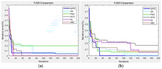
Figure 4.
The convergence curves in Case 1: (a) P1 instances and (b) P2 instances.
As we can see in Figure 4, in most cases, the proposed APPC made it easy to find the optimal solution through less iterative computation, and it entered into the error threshold 0.1% earlier. All swarm intelligence algorithms heuristically searched for the optimal solution, and the convergence curves varied. Because the scale of the P2 instances was greater than the P1 instances, all algorithms tended to need more iterative computation before finding the optimal solutions. With the help of a variable population size, the APPC acquired more stable performance when the problem scale increased.
5.3. Case 2: 10 Large-Sized Benchmark Instances
Case 2 was composed of 10 large-sized benchmark instances (SWV01–SWV10) for the job shop scheduling problem, where there are 20 jobs, 2 sets of machines, and 2 fleets [6,38]. Each job had 10 or 15 production operations. In all instances, the maximum operation number of each job equaled the maximum machine number. The benchmark provided two arbitrarily generated travel time matrices, where there were 10 and 15 machines in each machine set and 3 and 5 vehicles in each fleet [38]. Hence, Case 2 was a more serious challenge.
In Case 2, for the SWV01-SWV05 instances, jmax = 20, mmax = 10, and Ojmax = 10; for the SWV06-SWV10 instances, jmax = 20, mmax = 15, and Ojmax = 15. There were two fleets, and three and five vehicles in each fleet, that is, vmax = 3 or 5. The required processing time Pji of operation Oji on the machine m was randomly generated from the interval [1, 100], and the required transportation time Tji of an operation Oji on the vehicle v was arbitrarily generated from the interval [0, 42].
Table 3 and Table 4 show the optimal solutions for the 10 large-sized benchmark instances, where Table 3 has three vehicles and Table 4 has five vehicles. The “Ref” columns in Table 3 and Table 4 give the benchmark values from [38], which are the results of the constraint programming (CP2) integrating the pick-up and drop-off into a single-transfer task.
Table 3.
Optimal solutions in Case 2 (vmax = 3).
Table 4.
Optimal solutions in Case 2 (vmax = 5).
From the results in Table 3 and Table 4, it can be seen that the proposed APPC algorithm outperformed most swarm intelligence algorithms in 10 large-sized benchmark instances. The APPC made it easy to search for the optimal solutions from seven instances in Table 3 and eight instances in Table 4 among the 10 large-sized benchmark instances with three and five vehicle fleets, respectively. At the same time, the APPC algorithm obtained average deviations of 1.88% in Table 3 and 1.96% in Table 4 compared to Ref in [38] with three and five vehicle fleets, respectively, lower than other algorithms.
For the computation times, the proposed APPC algorithm needed less time to search for the optimal solutions. The APPC had great robustness in large-sized problem instances, where the total number of operations of all jobs increased from 6 × 6 and 10 × 10 in Case 1 to 20 × 15 and 20 × 15 in Case 2. The problem scale increased up to 8.33 times at most, while the average deviations of the APPC compared to the Ref in [37,38] were stable, with minimization of the makespan, processing waiting time, and the transportation waiting time. The rapid expansion of the problem scale did not lead to a sharp deterioration in the performance of the APPC algorithm.
To observe the time performance of these algorithms, the convergence curves are compared in Figure 5, including the proposed APPC, GA [2,4,16], PSO [6,19], ACO [8], DL [12,27], and ABC [13]. The maximum iterations were Ite_max = 200, and the error threshold was eth = 0.1%. As we can see in Figure 5, in most cases, the proposed APPC made it easy to find the optimal solution through less iterative computation, and it can enter into the error threshold 0.1% earlier.

Figure 5.
The convergence curves in Case 1: (a) SWV05 instance and (b) SWV10 instance.
Compared to the results in Figure 4, all swarm intelligence algorithms in Figure 5 required more iterative computation to search for the optimal solutions since the instances in Case 2 were large-sized and more complex than those of Case 1. Although the convergence curves varied, all algorithms tended to need more time in SWV10 than in SWV05 due to the greater problem scale of the SWV10 instances. With the help of the expansion and contraction operations, the APPC tended to be more stable than most algorithms when the problem scale increased. Other algorithms were also excellent to solve the FJSS problem, i.e., DL [12,27], but its computational time in each iteration was far longer than all algorithms. When the problem scale rapidly expanded, the solving time of DL [12,27] significantly increased.
5.4. Discussion and Comparison
For further analysis, a comparison of the average iterative errors and time performance are shown in Table 2. The comparison indexes include the solution error (%), makespan error (%), the error (%) of average processing waiting time WM, the error (%) of the average transportation waiting time WV, and the solving time (s). The proposed APPC was compared with a genetic algorithm (GA) [2,4,16], particle swarm optimization (PSO) [6,19], ant colony optimization (ACO) [8], deep learning (DL) [12,27], and artificial bee colony (ABC) [13].
As we can see in Table 5, these swarm intelligence algorithms obtained close average iterative errors on the main objectives, including the solution error (%), makespan error (%), the error (%) of the average processing waiting time WM, and the error (%) of the average transportation waiting time WV. The proposed APPC algorithm outperforms the other algorithms in most indexes. Here, the scale of the FJSS problem can be described as the product of three variables, i.e., the total number of jobs, machines, and vehicles. Case 1 selected nine P1 instances, sixteen P2 instances, and one fleet in total. Every P1 instance had 6 jobs, 6 operations, and 6 machines, and every P2 instance had 10 jobs, 10 operations, and 10 machines. The fleets in the P1 and P2 instances only considered a single vehicle. Case 2 selected 10 large-sized benchmark instances, where there were 20 jobs, each job had 10 or 15 production operations, 10 or 15 machines, and two fleets with 3 and 5 vehicles. Therefore, the problem scale in Case 1 was 6 × 6 × 1 = 36 of P1 and 10 × 10 × 1 = 100 of P2, and the problem scale in Case 2 was 20 × 10 × 3 = 600, 20 × 10 × 5 = 1000, 20 × 15 × 3 = 900, and 20 × 15 × 5 = 1500. Since the scale of the problems in Case 2 was greater than those in Case 1, the iterative error and computational time of all algorithms in Case 2 was worse than those in Case 1. For a swarm intelligence algorithm, the time performance is linearly related to its population size S and the scale of the job shop scheduling problem, including the maximum number of jobs, the maximum number of operations, the maximum number of machines, and the maximum number of vehicles. However, our proposed APPC algorithm acquired more stable performance when the problem scale increased. Although DL [12,27] has great searching capability, it consumes more computational time than most swarm intelligence algorithms since the time performance of DL [12,27] is related to the scale of the FJSS problem, the population size of the convolution cores, the number cin of input channels, and the number cout of output channels.
Table 5.
Performance comparison of multi-objective function.
According to the benchmark experimental results, it was verified that the proposed APPC algorithm has some merits in solving the FJSS problem with transportation constraints.
First, the proposed APPC algorithm can use the multi-objective function in Equations (1)–(15) to solve the FJSS problem with transportation constraints, rather than solving the job shop scheduling problem (JSSP) and transportation scheduling problem (TSP) separately. The APPC can use the multi-objective function as the fitness function to search for the optimal solutions.
Second, the variable population size of the proposed APPC algorithm can effectively improve its search performance. In the expansion operation, more mycelia are produced to search for more feasible solutions by self-learning, social learning, and free learning. Three parts of the mycelia can enhance global searching and local searching, and the population size increases.
Third, the optimal solutions are easy to preserve in the contraction of the proposed APPC algorithm so as to improve its convergence performance. In each iteration, the APPC uses a fast grouping section algorithm to select the best mycelium with high fitness, and the population size recovers. The contraction operation effectively protects the optimal solutions after expansion operation, but the other swarm intelligence algorithms are more likely to lose the optimal solution in each iteration. The expansion and contraction operations solve the problem well whereas for the traditional swarm intelligence algorithm, it is easy to fall into the local optimal solution prematurely.
Fourth, the FJSS problem with transportation constraints is an NP-hard problem, and traditional swarm intelligence algorithms tend to deteriorate rapidly with the expansion of the problem scale. Although the difficulty of integrating two subproblems is higher than solving them separately, the APPC algorithm can acquire a good balance between the solving accuracy and solving time. The time performance and space performance of the APPC are linearly correlated with the problem scale and computational parameters, so it is not easy for the solution performance to deteriorate as the scale of the problem increases.
Hence, the FJSS problem with transportation constraints can be well solved by the APPC algorithm, and the APPC algorithm has great potential for application in other NP-hard problems.
6. Conclusions
This paper addresses the flexible job shop scheduling problem with transportation constraints, which is more challenging than classic job scheduling problems. The problem involves two subproblems, i.e., the machine scheduling problem and the vehicle scheduling problem. Splitting the two subproblems may reduce the difficulty of solving them, but it cannot optimize the overall solution. This article attempts to integrate and optimize two subproblems at the same time. Since these two scheduling problems are NP-hard, their integrated problem is also NP-hard. Here, we built a state transition diagram, a multi-objective function, and constraints for the flexible job shop scheduling problem with transportation constraints. To effectively solve the complex FJSS problem, we proposed a novel artificial Physarum polycephalum colony algorithm based on the advantages and disadvantages of traditional swarm intelligence algorithms. The proposed APPC algorithm successfully simulates the unique behavioral characteristics of a natural Physarum polycephalum colony. It has a variable population size and searches for the optimal solutions to the FJSS problem by expansion and contraction operations. The benchmark experimental results on benchmark instances [6,37,38] revealed that the proposed APPC algorithm can achieve better performance than most traditional swarm intelligence algorithms.
The shortcomings of this work are that the problem only considered the minimization of the makespan, average processing waiting time, and average transportation waiting time. More engineering application indicators and real-world data have not been considered in this work, and many uncertain factors in scheduling are also lacking consideration, i.e., collision, deadlock, congestion, etc. To simplify the experiment, carpooling [39] and platooning [40] were not considered here so that the experiment could be completed more smoothly. Of course, these factors will make the problem more complex and difficult to solve, which will be one of our next research directions. In addition, natural Physarum polycephalum colonies can produce tens of thousands of mycelia to search the surrounding environment, which is difficult to simulate on personal computers, as it may cause computers to crash. How to better simulate the behavior of a Physarum polycephalum colony on personal computers is another research direction. Other interesting and meaningful issues may include mobile robots, electric vehicles, automatic routing, and so forth.
Author Contributions
Conceptualization, Z.C. and Y.F.; methodology, Z.C., Y.F. and S.Y.; validation, Y.F., S.Y. and J.Y.; writing—original draft preparation, Y.F.; writing—review and editing, Z.C., Y.F., S.Y. and J.Y.; supervision, Z.C. and Y.F.; project administration, Z.C. and Y.F.; funding acquisition, Z.C. All authors have read and agreed to the published version of the manuscript.
Funding
This research was funded by the National Natural Science Foundation of China (No. 71471102), Major Science and Technology Projects in Hubei Province of China (Grant No. 2020AEA012), and the Yichang University Applied Basic Research Project in China (Grant No. A17-302-a13).
Institutional Review Board Statement
This study did not require ethical approval.
Informed Consent Statement
Not applicable.
Data Availability Statement
Not applicable.
Acknowledgments
The authors give thanks to all of the anonymous reviewers for their hard work in helping to improve the quality of this submission.
Conflicts of Interest
The authors declare no conflict of interest.
References
- Abderrahim, M.; Bekrar, A.; Trentesaux, D.; Aissani, N.; Bouamrane, K. Bi-local search based variable neighborhood search for job-shop scheduling problem with transport constraints. Optim. Lett. 2022, 16, 255–280. [Google Scholar] [CrossRef]
- Homayouni, S.M.; Fontes, D.B.M.M.; Goncalves, J.F. A multistart biased random key genetic algorithm for the flexible job shop scheduling problem with transportation. Int. Trans. Oper. Res. 2023, 30, 688–716. [Google Scholar] [CrossRef]
- Homayouni, S.M.; Fontes, D.B.M.M. Production and transport scheduling in flexible job shop manufacturing systems. J. Glob. Optim. 2021, 79, 463–502. [Google Scholar] [CrossRef]
- Meng, L.L.; Cheng, W.Y.; Zhang, B.; Zou, W.Q.; Fang, W.K.; Duan, P. An improved genetic algorithm for solving the multi-AGV flexible job shop scheduling problem. Sensors 2023, 23, 3815. [Google Scholar] [CrossRef]
- Yao, Y.J.; Liu, Q.H.; Li, X.Y.; Gao, L. A novel MILP model for job shop scheduling problem with mobile robots. Robot. Comput. Integr. Manuf. 2023, 81, 102506. [Google Scholar] [CrossRef]
- Fontes, D.B.M.M.; Homayouni, S.M.; Goncalves, J.F. A hybrid particle swarm optimization and simulated annealing algorithm for the job shop scheduling problem with transport resources. Eur. J. Oper. Res. 2023, 306, 1140–1157. [Google Scholar] [CrossRef]
- Fontes, D.B.M.M.; Homayouni, S.M.; Resende, M.G.C. Job-shop scheduling-joint consideration of production, transport, and storage/retrieval systems. J. Comb. Optim. 2022, 44, 1284–1322. [Google Scholar] [CrossRef]
- Thiruvady, D.; Nguyen, S.; Shiri, F.; Zaidi, N.; Li, X.D. Surrogate-assisted population based ACO for resource constrained job scheduling with uncertainty. Swarm Evol. Comput. 2022, 69, 101029. [Google Scholar] [CrossRef]
- Fontes, D.B.M.M.; Homayouni, S.M.; Fernandes, J.C. Energy-efficient job shop scheduling problem with transport resources considering speed adjustable resources. Int. J. Prod. Res. 2023. [Google Scholar] [CrossRef]
- Yunusoglu, P.; Yildiz, S.T. Solving the flexible job shop scheduling and lot streaming problem with setup and transport resource constraints. Int. J. Syst. Sci. Oper. Logist. 2023, 10, 2221072. [Google Scholar] [CrossRef]
- Hajibabaei, M.; Behnamian, J. Fuzzy cleaner production in assembly flexible job-shop scheduling with machine breakdown and batch transportation: Lagrangian relaxation. J. Comb. Optim. 2023, 45, 112. [Google Scholar] [CrossRef]
- Yang, Z.; Bi, L.; Jiao, X.G. Combining reinforcement learning algorithms with graph neural networks to solve dynamic job shop scheduling problems. Processes 2023, 11, 1571. [Google Scholar] [CrossRef]
- Diaz, H.; Palacios, J.J.; Gonzalez-Rodriguez, I.; Vela, C.R. An elitist seasonal artificial bee colony algorithm for the interval job shop. Integr. Comput. Aided Eng. 2023, 30, 223–242. [Google Scholar] [CrossRef]
- Li, R.; Gong, W.Y.; Wang, L.; Lu, C.; Zhuang, X.Y. Surprisingly popular-based adaptive memetic algorithm for energy-efficient distributed flexible job shop scheduling. IEEE Trans. Cybern. 2023. early access. [Google Scholar] [CrossRef]
- Kippenberger, S.; Pipa, G.; Steinhorst, K.; Zoller, N.; Kleemann, J.; Ozistanbullu, D.; Ozistanbullu, D.; Scheller, B. Learning in the single-cell organism Physarum polycephalum: Effect of propofol. Int. J. Mol. Sci. 2023, 24, 6287. [Google Scholar] [CrossRef]
- Chaudhry, I.A.; Rafique, A.F.; Boudjemline, A. Integrated scheduling of machines and automated guided vehicles (AGVs) in flexible job shop environment using genetic algorithms. Int. J. Ind. Eng. Comput. 2022, 13, 343–362. [Google Scholar] [CrossRef]
- Wei, L.X.; He, J.X.; Guo, Z.Y.; Hu, Z.Y. A multi-objective migrating birds optimization algorithm based on game theory for dynamic flexible job shop scheduling problem. Expert Syst. Appl. 2023, 227, 120268. [Google Scholar] [CrossRef]
- Shim, S.O.; Jeong, B.; Bang, J.Y.; Park, J. Scheduling jobs with a limited waiting time constraint on a hybrid flowshop. Processes 2023, 11, 1846. [Google Scholar] [CrossRef]
- Zarrouk, R.; Ben Daoud, W.; Mahfoudhi, S.; Jemai, A. Embedded PSO for Solving FJSP on embedded environment (Industry 4.0 Era). Appl. Sci. 2022, 12, 2829. [Google Scholar] [CrossRef]
- Kong, X.H.; Yao, Y.H.; Yang, W.Q.; Yang, Z.L.; Su, J.Z. Solving the flexible job shop scheduling problem using a discrete improved grey wolf optimization algorithm. Machines 2022, 10, 1100. [Google Scholar] [CrossRef]
- Su, X.; Zhang, C.Y.; Ji, W.X. Dynamic configuration method of flexible workshop resources based on IICA-NS algorithm. Processes 2022, 10, 2394. [Google Scholar] [CrossRef]
- Song, H.C.; Liu, P. A study on the optimal flexible job-shop scheduling with sequence-dependent setup time based on a hybrid algorithm of improved quantum cat swarm optimization. Sustainability 2022, 14, 9547. [Google Scholar] [CrossRef]
- Sanogo, K.; Benhafssa, A.M.; Sahnoun, M.; Bettayeb, B.; Abderrahim, M.; Bekrar, A. A multi-agent system simulation based approach for collision avoidance in integrated job-shop scheduling problem with transportation tasks. J. Manuf. Syst. 2023, 68, 209–226. [Google Scholar] [CrossRef]
- Sun, J.C.; Xu, Z.F.; Yan, Z.H.; Liu, L.L.; Zhang, Y.X. An approach to integrated scheduling of flexible job-shop considering conflict-free routing problems. Sensors 2023, 23, 4526. [Google Scholar] [CrossRef]
- Liu, Q.H.; Wang, N.J.; Li, J.; Ma, T.T.; Li, F.P.; Gao, Z.J. Research on flexible job shop scheduling optimization based on segmented AGV. CMES-Comput. Model. Eng. Sci. 2023, 134, 2073–2091. [Google Scholar] [CrossRef]
- Cai, Z.; Zhang, Y.; Wu, M.; Cai, D. An entropy-robust optimization of mobile commerce system based on multi-agent system. Arab. J. Sci. Eng. 2016, 41, 3703–3715. [Google Scholar] [CrossRef]
- Inal, A.F.; Sel, C.; Aktepe, A.; Turker, A.K.; Ersoz, S. A multi-agent reinforcement learning approach to the dynamic job shop scheduling problem. Sustainability 2023, 15, 8262. [Google Scholar] [CrossRef]
- Cai, Z.; Xiong, Z.; Wan, K.; Xu, Y.; Xu, F. A node selecting approach for traffic network based on artificial slime mold. IEEE Access 2020, 8, 8436–8448. [Google Scholar] [CrossRef]
- Cai, Z.; Yang, Y.; Zhang, X.; Zhou, Y. Design a robust logistics network with an artificial Physarum swarm algorithm. Sustainability 2022, 14, 14930. [Google Scholar] [CrossRef]
- Ma, X.D.; Bi, L.; Jiao, X.G.; Wang, J.J. An efficient and improved coronavirus herd immunity algorithm using knowledge-driven variable neighborhood search for flexible job-shop scheduling problems. Processes 2023, 11, 1826. [Google Scholar] [CrossRef]
- Cai, Z.; Jiang, S.; Dong, J.; Tang, S. An artificial plant community algorithm for the accurate range-free positioning of wireless sensor networks. Sensors 2023, 23, 2804. [Google Scholar] [CrossRef] [PubMed]
- Cai, Z.; Ma, Z.; Zuo, Z.; Xiang, Y.; Wang, M. An image edge detection algorithm based on an artificial plant community. Appl. Sci. 2023, 13, 4159. [Google Scholar] [CrossRef]
- Zhang, S.J.; Gu, X.S. A discrete whale optimization algorithm for the no-wait flow shop scheduling problem. Meas. Control 2023. [Google Scholar] [CrossRef]
- Sahman, M.A.; Korkmaz, S. Discrete artificial algae algorithm for solving job-shop scheduling problems. Knowl. Based Syst. 2022, 256, 109711. [Google Scholar] [CrossRef]
- Xie, F.W.; Li, L.L.; Li, L.; Huang, Y.P.; He, Z.X. A decomposition-based multi-objective Jaya algorithm for lot-streaming job shop scheduling with variable sublots and intermingling setting. Expert Syst. Appl. 2023, 228, 120402. [Google Scholar] [CrossRef]
- Wen, X.Y.; Fu, Y.Z.; Yang, W.C.; Wang, H.Q.; Zhang, Y.Y.; Sun, C.Y. An effective hybrid algorithm for joint scheduling of machines and AGVs in flexible job shop. Meas. Control 2023. [Google Scholar] [CrossRef]
- Hurink, J.L.; Knust, S. Tabu search algorithms for job-shop problems with a single transport robot. Eur. J. Oper. Res. 2005, 162, 99–111. [Google Scholar] [CrossRef]
- Ham, A. Transfer-robot task scheduling in job shop. Int. J. Prod. Res. 2020, 59, 813–823. [Google Scholar] [CrossRef]
- Carrino, F.; Vaucher, Q.; Pasquier, R.; Bourquin, V.; Khaled1, O.A.; Mugellini, E.; Gobron, S. Bombuscar: Gamification design of a carpolling-based freight transport. In Proceedings of the GSGS’20: 5th Gamification & Serious Game Symposium, Online, 24 September–5 November 2020. [Google Scholar]
- Wiseman, Y. Intelligent transportation systems along with the COVID-19 pandemic will significantly change the transportation market. Open Transp. J. 2021, 15, 11–15. [Google Scholar] [CrossRef]
Disclaimer/Publisher’s Note: The statements, opinions and data contained in all publications are solely those of the individual author(s) and contributor(s) and not of MDPI and/or the editor(s). MDPI and/or the editor(s) disclaim responsibility for any injury to people or property resulting from any ideas, methods, instructions or products referred to in the content. |
© 2023 by the authors. Licensee MDPI, Basel, Switzerland. This article is an open access article distributed under the terms and conditions of the Creative Commons Attribution (CC BY) license (https://creativecommons.org/licenses/by/4.0/).