Research on Path Tracking and Yaw Stability Coordination Control Strategy for Four-Wheel Independent Drive Electric Trucks

Abstract

Achieving accurate path tracking and vehicle stability control for four-wheel independent drive electric trucks under complex driving conditions, such as high speed and low adhesion, remains a major challenge in current research. Poor coordination control may cause the vehicle to deviate from its intended path and become unstable. To address this issue, this article proposes a coordinated control strategy consisting of a three-layer control framework. In the upper layer controller design, establish a linear quadratic regulator (LQR) path tracking controller to ensure precise steering control by eliminating steady-state errors through feedforward control. The middle layer controller utilizes the fractional order sliding mode control (FOSMC) yaw moment controller to calculate the additional yaw moment based on the steering angle of the upper input, utilizing the error of yaw rate and sideslip angle as the state variable. To collectively optimize the control system, establish a coordinated optimization objective function and utilize the hybrid genetic-particle swarm optimization algorithm (GA-PSO) to optimize the weight coefficient of LQR and sliding mode parameters of FOSMC, effectively improving the performance of the controller. In the lower layer torque distribution controller, use the quadratic programming method to achieve real-time optimal torque distribution based on tire utilization, which improves vehicle stability control. Through simulations conducted under four different working conditions, the proposed control scheme demonstrates a 15.54% to 23.17% improvement in tracking performance and a 10.83% to 23.88% optimization in vehicle driving stability compared to other control methods. This scheme provides a theoretical reference for path tracking and stability control in four-wheel independent drive electric trucks.

1. Introduction

With the increasing number of vehicles, issues such as traffic congestion and vehicle safety have gained significant attention [1,2,3]. Additionally, the field of artificial intelligence has made significant progress, leading to the emergence of intelligent vehicles with autonomous driving capabilities, which have become a global research focus over the past decade [4,5]. Path tracking control is a vital technology in automotive intelligence. It ensures that vehicles stay on the intended path by controlling the angle of the front wheels in real time [6,7,8]. Four-wheel independent drive electric vehicles have garnered significant interest in autonomous driving research due to their high flexibility, maneuverability, and efficient transmission [9,10,11]. However, the unique dynamic characteristics and redundant configuration of these vehicles present challenges in terms of chassis control [12]. Consequently, achieving path tracking accuracy and stability in complex conditions while leveraging the advantages of independent torque control poses a crucial challenge.

The primary objective of path tracking control in vehicle systems is to accurately follow a reference path by eliminating tracking bias. Numerous path tracking control strategies have been proposed by researchers, such as Proportional Integral Differential (PID) control [13,14], fuzzy control [15], Sliding Mode Control (SMC) [16], Model Predictive Control (MPC) [17], feedback feedforward control [18,19], and Linear Quadratic Regulator (LQR) control [20]. Among these methods, LQR is widely utilized in vehicle lateral control due to its simplicity in design, ease of implementation, and robustness against uncertainties [21]. However, due to the existence of system steady-state errors, the tracking control accuracy of the LQR method is limited. In order to address this limitation, Zhao et al. [22] proposed a motion control method using LQR with feedforward control, effectively eliminating lateral steady-state errors in path tracking. Li et al. [23] suggested an improved LQR control by incorporating an enhanced path planning algorithm. This involved applying the path optimization solution method to construct feedforward feedback LQR control, and solving the real-time path planning information and control input parameters to minimize tracking errors. Xu et al. [24] augmented LQR feedback control with path curvature feedforward control to reduce steady-state deviation of the controller. Another study [25] proposed a Linear-Quadratic Regulator that combines feedback and feedforward mechanisms to maintain vehicle stability within the handling limit while minimizing path deviation. Nonetheless, the weight determination for the Linear-Quadratic Regulator is typically performed empirically, making it cumbersome and inefficient when encountering changing environments. Thus, Ni et al. [26] designed an improved Self-tuning Weighting Matrix Linear-Quadratic Regulator, which integrates feedforward control to achieve lateral motion control and enhance path tracking accuracy. Additionally, Wang et al. [27] proposed a lateral path control strategy based on an enhanced LQR algorithm. This approach dynamically adjusts the weight coefficients of LQR using fuzzy control in response to the vehicle’s status, resulting in improved tracking accuracy, steering stability, and computational efficiency. Furthermore, Lu et al. [28] introduced an adaptive LQR path tracking controller that optimizes the LQR weight matrix utilizing genetic algorithms (GA), thereby effectively enhancing tracking accuracy and vehicle stability. While previous studies have shown promising results in enhancing the LQR algorithm, there is still potential for further improvement in terms of control accuracy and stability. Lei et al. [29] improved the effectiveness of the articulated vehicle winding oscillation controller by optimizing each parameter in the LQR controller through Particle Swarm Optimization (PSO). The GA-PSO algorithm combines the advantages of the GA and PSO and demonstrates strong performance in solving complex optimization problems. The GA explores the optimal solution space through selection, crossover, and mutation operations, while PSO emulates the behavior of a particle swarm to identify the optimal solution. By combining these two algorithms, the GA-PSO algorithm achieves a balance between global and local searches, resulting in improved search efficiency, higher-quality optimization results, and more effective resolution of optimization problems.

Previous research has primarily focused on path tracking for autonomous vehicles under traditional driving systems, with the steering angle being the only output of lateral control. However, in four-wheel independent drive vehicles, the redundant control output, known as additional yaw torque generated through the torque difference between the left and right wheel motors, can significantly enhance turning performance and driving stability of the vehicle [30,31,32]. Comparative analysis by reference [33] demonstrates that compared to vehicles using only front wheel steering, four-wheel independent drive vehicles have a much wider achievable range for tracking control. Scholars have proposed various schemes for combining path tracking control and yaw stability control in four-wheel independent drive vehicles, mainly in centralized and distributed structures [34]. Centralized structures typically integrate vehicle stability parameters, including yaw rate and center of mass sideslip angle, into the vehicle path tracking control model. It employs the additional yaw moment or longitudinal force from each wheel as the control variable and solves it in conjunction with the front wheel angle. Reference [35] adopts an adaptive robust linear quadratic tuning controller to achieve the optimal active front wheel steering and direct yaw torque control inputs, while considering vehicle lateral stability and eliminating the effects of parameter uncertainty. In reference [36], Model Predictive Control technology is employed to simultaneously determine the optimal front wheel steering angle and external yaw moment, ensuring the required path tracking performance and lateral stability of the vehicle. However, in the centralized scheme mentioned above, no matter how stable the vehicle is during the tracking process, additional driving or braking force will be applied to both wheels. Due to the continuous generation of additional driving or braking force on the vehicle, this not only fails to ensure optimal path tracking performance, but also leads to unnecessary energy consumption due to continuous control. In distributed structures, path tracking control and stability control controllers are usually designed separately. It can effectively solve the above problems and achieve better control. To enhance the overall performance of autonomous vehicles, reference [37] proposes a coordinated control of yaw torque tracking deviation compensation and vehicle stability to improve tracking accuracy and stability. MPC is used to calculate front wheel steering angle, enabling the vehicle to follow the reference path through autonomous steering. Simultaneously, an active yaw torque-based SMC controller calculates and distributes the yaw torque according to the vehicle’s constant torque requirements for stability control. Sliding mode control has good disturbance attenuation capability. However, due to the adoption of traditional reaching law, the inherent chattering problem has not been fundamentally resolved [38,39]. In terms of sliding surface design, compared to integer-order sliding surfaces, fractional-order sliding surfaces have slower convergence rates for calculus operators. Including fractional-order sliding surfaces in the design of sliding mode can store motion parameters and enhance control tracking and disturbance suppression capabilities. Therefore, they are widely used by researchers in different fields. Gudey et al. [40] proposes a fractional order sliding control (FOSMC) technique to reduce torque and flux ripple operating at fixed switching frequencies. Alebi et al. [41] designed a new fractional sliding mode controller for precise speed control of permanent magnet synchronous motors to track desired commands more quickly. Al-Dhaifallah et al. [42] indicated that proposing a new fractional-order sliding mode control approach to control the quadrotor working under a complex environment will likely increase the system’s control precision with high robustness and accuracy. Based on the literature mentioned, both centralized and distributed control structures utilize additional yaw moments to enhance path tracking performance while considering vehicle stability. However, for four-wheel independent drive trucks, the complexity of the vehicle increases. Further investigation is needed to improve the coordination strategy for vehicle driving stability while ensuring accurate vehicle path tracking. By deconstructing the calculation of steering and additional yaw moment and dividing it into upper and middle layers for separate calculations, hierarchical control can be further simplified, system calculation costs can be reduced, system stability can be enhanced, and a new three-layer structure can be established by combining torque distribution in the lower layer.

Therefore, this article proposes a path tracking and yaw stability coordinated control strategy based on four-wheel independent drive electric trucks, and verifies its good performance in path tracking and stability control through simulation under different operating conditions. The main contributions of this article are as follows. Firstly, a hierarchical control framework is established to achieve coordinated control of path tracking and yaw stability, including an upper layer LQR path tracking controller, a middle layer FOSMC yaw stability controller, and a lower layer torque optimization allocation controller; secondly, for the chattering problem of the original SMC, the fractional order operator and the improved reaching law are introduced to optimize, and the weight matrix of the original LQR and the sliding mode parameters of the FOSMC are solved by the hybrid genetic Particle Swarm Optimization (GA-PSO) algorithm, which improves the path tracking performance and vehicle yaw stability. Thirdly, based on the minimum objective function of tire utilization, the quadratic programming method is used to realize the optimal torque distribution problem, which ensures the driving stability of the four-wheel independent drive electric truck. Finally, the effectiveness and superiority of the proposed path tracking and yaw stability coordinated control strategy were verified under different operating conditions using the MATLAB/Simulink-TruckSim joint simulation platform.

The rest of this article is organized as follows. Section 2 introduces the modeling of vehicle dynamics. Section 3 elaborates on the path tracking and yaw stability coordination control strategy based on hierarchical control. Section 4 presents simulation results and discusses the effectiveness of the proposed strategy. Finally, Section 5 provides conclusions and prospects.

2. Vehicle Model

This article mainly establishes a two-degree-of-freedom (2DOF) vehicle model and a seven-degree-of-freedom (7DOF) vehicle model, among which the 2DOF vehicle model is mainly used to calculate the ideal values of the center of mass sideslip angle and yaw rate, as well as for use in path tracking controllers. The 7DOF vehicle model is mainly used to calculate the additional yaw moment and torque distribution. In path tracking control, the centroid sideslip angle and yaw rate are key state variables used to describe the lateral motion behavior of vehicles. The 2DOF vehicle model can already provide sufficient information to describe the lateral motion of the vehicle and has good control effects on yaw rate and center of mass sideslip angle.

However, when it comes to calculating the additional yaw moment and four-wheel torque distribution of the vehicle, using the 7DOF vehicle model may be more appropriate. The 7DOF vehicle model considers more details and complexity, including factors such as longitudinal and lateral acceleration, sideslip angle, and body posture of the vehicle. The use of the 7DOF model can more accurately describe the vehicle’s motion behavior and provide more detailed dynamic information, including additional yaw torque and four-wheel torque distribution.

2.1. 2DOF Vehicle Reference Model

The simplified 2DOF model is widely used for studying vehicle dynamics. Therefore, this study adopts a 2DOF vehicle dynamics model as the reference model for the controller. Considering the characteristics of distributed drive vehicles, a vehicle model is established that accounts for both lateral and yaw motions. According to [43], It is assumed that the longitudinal velocity at the center of gravity remains constant, and the sideslip angles of the wheels are small. The left and right wheels are treated as a single entity, effectively capturing the vehicle’s lateral and yaw motions. Our research mainly focuses on the driving conditions of vehicles under low lateral acceleration conditions. In this case, the behavior of the tire can be modeled and analyzed using a linear model with good approximation. The model is illustrated in Figure 1. Furthermore, the dynamic equation is established according to Equation (1).

$$\left\{\begin{array}{l}m{v}_x(\dot{\beta }+\omega )=F_{yf}\cos \delta +F_{yr}\hfill \\ I_z\dot{\omega }=a{F}_{yf}\cos \delta +b{F}_{yr}\hfill \end{array}\right.$$

(1)

where $m$ is the mass of the vehicle, $v_x$ is the longitudinal speed of the vehicle, $\delta$ is the angle of the front wheel of the vehicle, $\omega$ and $\beta$ are respectively the yaw rate and the sideslip angle of the center of mass of the vehicle, $F_{yf}$ and $F_{yr}$ are respectively the cornering forces generated by the front and rear wheels, $I_z$ is the Moment of inertia of the vertical axis of the vehicle around the center of mass, $a$ and $b$ are respectively the distance from the center of mass of the vehicle to the front and rear axles, and $\Delta M_z$ is the additional yaw moment of the vehicle.

Based on the assumption that the sideslip angle of each wheel is small, it can be concluded that

$$\left\{\begin{array}{l}{F}_{yf}=C_f{\alpha }_f=C_f\left(\delta -\beta -\frac{a\omega }{v_x}\right)\\ F_{yr}=C_r{\alpha }_r=C_r\left(\frac{b\omega }{v_x}-\beta \right)\end{array}\right.$$

(2)

where $C_f$ and $C_r$ represent the lateral stiffness of the front and rear axle wheels, respectively, while ${\alpha }_f$ and ${\alpha }_r$ represent the lateral angles of the front and rear wheels, respectively.

By combining Equations (1) and (2), it can be concluded that

$$\left\{\begin{array}{l}\dot{\beta }=\frac{C_f+C_r}{m{v}_x}\beta +\left(\frac{a{C}_f-b{C}_r}{m{v}_x^2}-1\right)\omega -\frac{C_f}{m{v}_x}\delta \hfill \\ \dot{\omega }=\frac{a{C}_f-b{C}_r}{I_z}\beta +\frac{a^2{C}_f+b^2{C}_r}{I_z{v}_x}\omega -\frac{a{C}_f}{I_z}\delta \hfill \end{array}\right.$$

(3)

2.2. Vehicle State Reference Value

When the vehicle is in a stable driving state, it should meet the requirements of $\dot{\beta }=0$ and $\dot{\omega }=0$, which can be obtained by combining Equation (3)

$$\begin{array}{cc}{\omega }_d=\frac{v_x}{L(1+K{v}_x^2)}& ,K=\frac{m}{L^2}\left(\frac{a}{C_r}-\frac{b}{C_f}\right)\end{array}$$

(4)

where ${\omega }_d$ is the ideal yaw rate, $K$ is the vehicle stability factor, and $L=a+b$ is the vehicle wheelbase.

Moreover, it is crucial to acknowledge that the vehicle’s maximum lateral acceleration is constrained by the road adhesion coefficient [44], as outlined in Equation (5).

$$a_y\le \mu g$$

(5)

where $a_y$ is the lateral acceleration of the vehicle, $\mu$ is the road adhesion coefficient, and $g=9.8 \mathrm{m}/{\mathrm{s}}^2$ is the Gravitational acceleration.

The reference value of yaw rate that satisfies the constraint can be expressed as Equation (6).

$${\omega }_d=\min \left\{\left|\frac{v_x}{L(1+K{v}_x^2)}\delta \right|,\left|\frac{\mu g}{v_x}\right|\right\}\mathrm{sign}(\delta )$$

(6)

The sideslip angle, denoting the difference between the direction of vehicle travel and the direction of the front of the vehicle, is measured at the center of mass. Minimizing this angle contributes to enhancing the vehicle’s lateral stability and reducing its lateral slip [45]. The reference value for the vehicle’s sideslip angle is defined as follows.

$${\beta }_d=0$$

(7)

2.3. 7DOF Vehicle Dynamics Model

Due to the vehicle system being a highly nonlinear system with multiple degrees of freedom, it is necessary to consider a significant amount of actual nonlinear external disturbances, rendering the 2DOF model no longer applicable. In order to reflect the vehicle model comprehensively and accurately under actual operating conditions, this paper establishes a 7DOF vehicle dynamics model as shown in Figure 2, where the seven degrees of freedom include longitudinal motion, lateral motion, yaw motion, and the rotational motion of the four wheels. The equations of motion are as follows.

The longitudinal equations of motion of the vehicle can be expressed as Equation (8),

$$m{a}_x=m({\dot{v}}_x-v_y\omega )=(F_{xfl}+F_{xfr})\cos \delta -(F_{yfl}+F_{yfr})\sin \delta +F_{xrl}+F_{xrr}$$

(8)

The lateral equations of motion of the vehicle can be expressed as Equation (9),

$$m{a}_y=m({\dot{v}}_y-v_x\omega )=(F_{xfl}+F_{xfr})\sin \delta +(F_{yfl}+F_{yfr})\cos \delta +F_{yrl}+F_{yrr}$$

(9)

The vehicle yaw equations of motion can be expressed as Equation (10),

$$\left\{\begin{array}{l}{I}_z\dot{\omega }=a(F_{yfl}+F_{yfr})\cos \delta -b(F_{yrl}+F_{yrr})+\frac{d_f}{2}(F_{yfr}-F_{yfl})\sin \delta +\Delta M_z\\ \Delta M_z=a(F_{xfl}+F_{xfr})\sin \delta +\frac{d_f}{2}(F_{xfr}-F_{xfl})\cos \delta +\frac{d_r}{2}(F_{xrr}-F_{xrl})\end{array}\right.$$

(10)

The equations of motion of wheel rotation can be expressed as Equation (11),

$$\begin{array}{cc}{J}_{\omega }{\dot{\omega }}_i=T_i-F_{xi}{R}_e& ,i=fl,fr,rl,rr\end{array}$$

(11)

where $v_y$ is the lateral speed of the vehicle, $d_f$ and $d_r$ are the track widths of the front and rear axles of the vehicle, respectively, $F_x$ and $F_y$ are the longitudinal force and lateral force of the vehicle, respectively, corner marks $fl$, $fr$, $rl$ and $rr$ represent the positions of the four wheels of the vehicle at the front left, front right, rear left, and rear right, respectively, $J_{\omega }$ is the Moment of inertia of the wheel, ${\omega }_i$ is the angular speed of the wheel, $T_i$ is the driving or braking torque acting on the wheel, and $R_e$ is the effective rolling radius of the wheel.

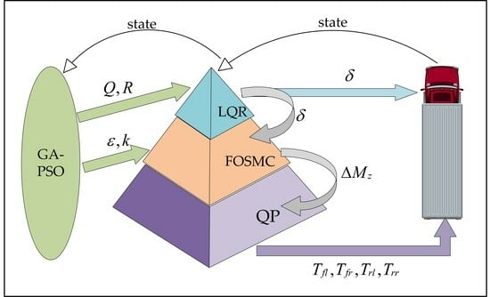
3. Coordinated Control Strategy for Path Tracking and Yaw Stability

This paper presents a hierarchical control strategy for coordinated path tracking and yaw stability in four-wheel independent drive electric trucks, as illustrated in Figure 3. In contrast to the traditional two-layer control framework, the hierarchical control framework proposed here consists of three layers. The upper layer is the path tracking control layer, which incorporates an LQR path tracking controller and a GA-PSO weight optimization algorithm. The GA-PSO algorithm optimizes the weight matrix of the LQR algorithm to track the desired path and calculates the front wheel angle based on the road deviation information at the preview point. This information is then used to compensate for the vehicle’s front wheel angle through feedforward control. Consequently, the required front wheel angle is determined, serving as an input to the middle layer controller. The middle layer, referred to as the yaw stability control layer, is composed of FOSMC and GA-PSO parameter optimization algorithms. By assessing the deviation between the current driving state and the reference state, the GA-PSO algorithm optimizes the parameters of FOSMC, facilitating the calculation of the additional yaw moment required to restore vehicle stability. This value is then conveyed to the lower layer controller. The lower layer, known as the torque distribution layer, involves the implementation of the PID longitudinal controller. The PID controller computes the total driving force based on the discrepancy between the actual vehicle speed and the target vehicle speed. It combines this information with the additional yaw torque computed by the yaw stability controller in the middle layer. The objective of this integration is to maximize tire utilization. Moreover, considering the constraints imposed by road adhesion conditions and the performance of the drive motor, the torque distribution is optimized to determine the torque allocation for all four wheels. This optimized torque is then applied to the vehicle, aiming to ensure accurate vehicle path tracking control while enhancing driving stability and safety.

3.1. Design of Upper Layer Path Tracking Controller

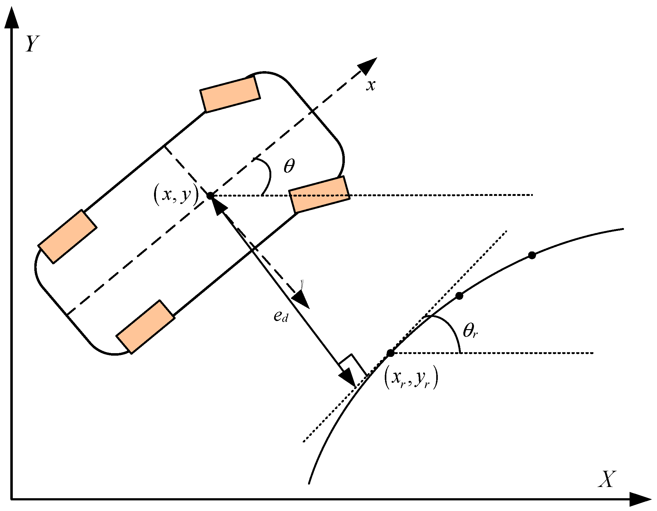
3.1.1. Vehicle Path Tracking Model

Combining the two-degree-of-freedom vehicle dynamics differential equation in Equation (3) and defining $\dot{y}=v_y$, the vehicle path tracking model can be obtained by rewriting the path tracking part, as shown in Equation (12).

$$\left(\begin{array}{l}\ddot{y}\hfill \\ \ddot{\phi }\hfill \end{array}\right)=\left(\begin{array}{ll}\frac{C_f+C_r}{m{v}_x}\hfill & \frac{a{C}_f-b{C}_r}{m{v}_x}-v_x\hfill \\ \frac{a{C}_f-b{C}_r}{I_z{v}_x}\hfill & \frac{a^2{C}_f+b^2{C}_r}{I_z{v}_x}\hfill \end{array}\right)\left(\begin{array}{l}\dot{y}\hfill \\ \dot{\phi }\hfill \end{array}\right)+\left(\begin{array}{c}-\frac{C_f}{m}\\ -\frac{a{C}_f}{I_z}\end{array}\right)\delta$$

(12)

where $\phi$ is the vehicle’s yaw angle; y is the lateral displacement.

3.1.2. Path Tracking Error Model

The tracking error model is illustrated in Figure 4. During the vehicle’s tracking of the reference path, there are primarily two deviations in path tracking: the lateral error $e_d$, which is the difference between the vehicle’s centroid position $\left(x,y\right)$ and the closest point position $\left(x_r,y_r\right)$ on the reference path, and the heading deviation $e_{\theta }$, which is the difference between the vehicle’s centroid position heading angle $\theta$ and the reference heading angle ${\theta }_r$.

Due to $e_{\theta }=\theta -{\theta }_r$ and for ease of calculation, based on the ideal vehicle centroid slip angle $\beta =0$ mentioned earlier, and because $\theta =\phi +\beta$, the two path tracking errors can be expressed as Equation (13).

$$\left\{\begin{array}{l}{e}_d=(x-x_r)n_r\\ e_{\phi }=\phi -{\theta }_r\end{array}\right.$$

(13)

where $n_r$ is the normal vector of the nearest point.

In practical control, designing a real-time controller is necessary to eliminate these two errors, enabling the vehicle to track and plan its path continuously. Calculating the first derivatives ${\dot{e}}_d$ and ${\dot{e}}_{\phi }$, and the second derivatives ${\ddot{e}}_d$ and ${\ddot{e}}_{\phi }$ of the lateral error $e_d$ and heading angle error $e_{\phi }$.

$$\left\{\begin{array}{l}{\dot{e}}_d=v_x{e}_{\phi }+v_y\\ {\dot{e}}_{\phi }\approx \dot{\phi }-{\rho }_r{v}_x\\ {\ddot{e}}_d=v_x{\dot{e}}_{\phi }+{\dot{v}}_y\\ {\ddot{e}}_{\phi }\approx \ddot{\phi }\end{array}\right.$$

(14)

where ${\rho }_r$ is the curvature of the nearest point.

The relationship between lateral error and heading error during vehicle steering can be obtained by combining Equation (12) with Equation (14), as shown in Equation (15).

$$\begin{array}{ll}\left[\begin{array}{l}{\dot{e}}_d\\ {\ddot{e}}_d\\ {\dot{e}}_{\phi }\\ {\ddot{e}}_{\phi }\end{array}\right]& =\left[\begin{array}{cccc}0& 1& 0& 0\\ 0& \frac{C_f+C_r}{m{v}_x}& -\frac{C_f+C_r}{m}& \frac{a{C}_f-b{C}_r}{m{v}_x}\\ 0& 0& 0& 1\\ 0& \frac{a{C}_f-b{C}_r}{I_z{v}_x}& -\frac{a{C}_f-b{C}_r}{I_z}& \frac{a^2{C}_f+b^2{C}_r}{I_z{v}_x}\end{array}\right]\left[\begin{array}{c}{e}_d\\ {\dot{e}}_d\\ e_p\\ {\dot{e}}_{\phi }\end{array}\right]\\ & +\left[\begin{array}{c}0\\ -\frac{C_f}{m}\\ 0\\ -\frac{a{C}_f}{I_z}\end{array}\right]\delta +\left[\begin{array}{c}0\\ \frac{a{C}_f-b{C}_r}{m{v}_x}-v_x\\ 0\\ \frac{a^2{C}_f+b^2{C}_r}{I_z{v}_x}\end{array}\right]{\dot{\theta }}_r\end{array}$$

(15)

Express Equation (15) in the form of the state space equation shown in Equation (16).

$$\dot{X}=AX+Bu+C{\dot{\theta }}_r$$

(16)

3.1.3. Preview Model

Path tracking control is a compensatory control based on the current path tracking error. There is a lag in the vehicle’s motion state. In order to comply with the habitual direction control during actual driving and reduce vehicle instability caused by repetitive adjustment of the front wheel angle due to control response lag, introduce a lookahead model to replace the information from the original vehicle sensor for subsequent control. By setting the lookahead time as $t_s$, it can obtain the lookahead point position information in Equation (17).

$$\left\{\begin{array}{l}{x}_{pre}=x+(v_x\cos \phi -v_y\sin \phi )t_s\\ y_{pre}=y+(v_x\sin \phi +v_y\cos \phi )t_s\\ {\phi }_{pre}=\phi +\dot{\phi }{t}_s\end{array}\right.$$

(17)

where $x_{pre}$ is the horizontal coordinate of the preview point, $y_{pre}$ is the vertical coordinate of the preview point, and ${\phi }_{pre}$ is the yaw angle of the preview point.

3.1.4. Design of LQR Controller

Since discrete path points are common in practical applications, opt for discrete LQR control. To design a discrete LQR, Equation (16) is discretized using the forward Euler method to derive the discrete vehicle tracking error state space equation. In the state space equation, the term $C{\dot{\theta }}_r$ is related to the path. Here, we decouple the rotation angle calculation problem, and the final rotation angle is equal to the sum of the rotation angle calculated based on the error and the additional rotation angle controlled by curvature feedforward when the path is assumed to be a straight line. Therefore, in the LQR problem, assuming the reference trajectory is a straight line, the radius R is infinite, the expected curvature is infinitely small, and the state space constant term $C{\dot{\theta }}_r$ can be ignored. In Section 3.1.5, a compensation will be implemented through feedforward control. The state equation is transformed into the following form:

$$X_{k+1}=\overline{A}{X}_k+\overline{B}{u}_k$$

(18)

where $\overline{A}={\left(I-\frac{Adt}{2}\right)}^{-1}\left(I+\frac{Adt}{2}\right)$; $\overline{B}=Bdt$.

LQR aims at minimizing the performance objective function by solving the corresponding Riccati Equation under given constraints, in order to obtain the optimal feedback control for the vehicle [46]. The objective of the LQR controller is to reduce the path tracking error of the vehicle and keep the control quantities as small as possible to ensure vehicle stability. Therefore, the following objective function is defined,

$$\min \mathrm{J}={\displaystyle \sum _{k=0}^{\infty }\left(X_k^{T}Q{X}_k+u_k^{T}R{u}_k\right)}, \left\{\begin{array}{l}Q=\mathrm{diag}\left[q_1,q_2,q_3,q_4\right]\\ R=\left[q_5\right]\end{array}\right.$$

(19)

where $X$ is the state variable of the system, $U$ is the control variable of the system, $Q$ is the weighted matrix of the state error indicating the degree of importance to the control objective, and $R$ is the weight matrix of the control quantity. $q_1,q_2,q_3,q_4$ represents the weight coefficients of lateral error, lateral error change rate, heading error, and heading error change rate; $q_5$ is the weight coefficient of the front wheel angle. The weight coefficient represents the importance of this variable. The larger the value, the faster the corresponding state variable converges.

The control law of LQR feedback control is as follows:

$$u_k=-K_{LQR}{X}_k$$

(20)

where $K_{LQR}=\left[K_1,K_2,K_3,K_4\right]$ is the gain coefficient of LQR controller, as shown in Equation (21).

$$K_{LQR}={\left(R+{\overline{B}}^{T}P\overline{B}\right)}^{-1}{\overline{B}}^{T}P\overline{A}$$

(21)

where matrix $P$ can be obtained by solving Riccati Equation.

$$P=Q-{\overline{A}}^{T}P\overline{B}{\left(R+{\overline{B}}^{T}P\overline{B}\right)}^{-1}{\overline{B}}^{T}P\overline{A}+{\overline{A}}^{T}P\overline{A}$$

(22)

3.1.5. Feedforward Control

Combining Equations (16) and (20), the system equation of state based on LQR feedback control can be obtained.

$$\dot{X}=(A-B{K}_{LQR})X+C{\dot{\theta }}_r$$

(23)

Due to the existence of the non-zero term $C{\dot{\theta }}_r$, regardless of the value of $K_{LQR}$, $\dot{X}$ and $X$ cannot both be zero. If only LQR feedback control is used, the system will always have steady-state errors; Therefore, in order to eliminate steady-state errors, a feedforward control variable ${\delta }_{ff}$ is introduced to remove the influence of the $C{\dot{\theta }}_r$ term, and the system control variable is

$$u=-K_{LQR}X+{\delta }_{ff}$$

(24)

In this case, let $\dot{X}=0$ and combining Equations (16) and (24), the state variables of the system without steady-state error can be obtained.

$$X=-{(A-B{K}_{LQR})}^{-1}\left(B{\delta }_{ff}+C{\dot{\theta }}_r\right)$$

(25)

From Equation (25), it can be derived that in order to achieve zero steady-state error in the system, i.e., $X=0$, and thus attain optimal control performance, it is necessary to calculate an appropriate value for ${\delta }_{ff}$. Combined with Equation (15), the equation representing the steady-state error of the system can be calculated as shown in Equation (26).

$$\left[\begin{array}{c}{e}_d\\ {\dot{e}}_d\\ e_{\phi }\\ {\dot{e}}_{\phi }\end{array}\right]=\left[\begin{array}{c}\frac{1}{K_1}\left\{{\delta }_{ff}-\frac{{\dot{\theta }}_r}{v_x}\left[a+b-b{K}_3-\frac{m{v}_x^2}{a+b}\left(\frac{b}{C_f}+\frac{a}{C_r}{K}_3-\frac{a}{C_r}\right)\right]\right.\\ 0\\ -\frac{{\dot{\theta }}_r}{v_x}\left(b+\frac{a}{a+b}\frac{m{v}_x^2}{C_r}\right)\\ 0\end{array}\right]$$

(26)

Due to the ideal vehicle center of gravity sideslip angle $\beta =0$, the vehicle yaw angle error can be represented as $e_{\phi }=\phi -{\theta }_r$ and $e_{\theta }=\phi +\beta -{\theta }_r=0$. Therefore, the yaw error can be directly eliminated. If want to eliminate the lateral error $e_d=0$, the feedforward control variable is ${\delta }_{ff}$.

$${\delta }_{ff}={\rho }_r\left[a+b-b{K}_3-\frac{m{v}_x^2}{a+b}\left(\frac{b}{C_f}+\frac{a}{C_r}{K}_3-\frac{a}{C_r}\right)\right]$$

(27)

3.2. Design of Middle Layer Stability Controller

Due to the slow convergence of fractional calculus operators, incorporating them into the design of sliding surfaces allows for the memory of motion parameters and enhances control tracking and disturbance rejection. By adjusting the parameters of fractional calculus operators, the dynamic characteristics of systems can be described and controlled more accurately, enabling more precise reference signal tracking. Additionally, sliding mode control suffers from the inherent phenomenon of chattering [47]. Utilizing the slow decay property of fractional order systems over time can effectively suppress system oscillations. Therefore, introducing fractional calculus operators into sliding surfaces in nonlinear and time-varying systems can improve the system’s disturbance rejection capability, tracking accuracy, and stability, thereby achieving better control performance. Design a sliding surface that combines the impact of vehicle yaw rate and center of mass sideslip angle on vehicle stability,

$$s=c_{{}_1}{e}_{\omega }+D^{\lambda }{e}_{\omega }+c_2{\dot{e}}_{\beta }+D^{\lambda }{e}_{\beta }, \left\{\begin{array}{l}{e}_{\omega }={\omega }_d-\omega \\ e_{\beta }={\beta }_d-\beta \end{array}\right.$$

(28)

where $e_{\omega }$ and $e_{\beta }$ are the tracking errors of yaw rate and center of mass sideslip angle, respectively. $c_{{}_1}$ and $c_2$ are the weight coefficients of yaw rate error and center of mass sideslip angle error, respectively. In this paper, the values are both 0.5, $D^{\lambda }$ is the fractional order calculus operator, and $\lambda$ is the fractional order calculus order. In this paper, the values are 0.2.

Taking the derivative of Equation (28) yields the first-order derivative of the sliding surface.

$$\dot{s}=c_{{}_1}{\dot{e}}_{\omega }+D^{\lambda }{\dot{e}}_{\omega }+c_2{\dot{e}}_{\beta }+D^{\lambda }{\dot{e}}_{\beta }, \left\{\begin{array}{l}{\dot{e}}_{\omega }={\dot{\omega }}_d-\dot{\omega }\\ {\dot{e}}_{\beta }={\dot{\beta }}_d-\dot{\beta }\end{array}\right.$$

(29)

Considering that the control amount is the additional yaw moment, combined with Equation (10), Equation (29) can be represented as Equation (30).

$$\begin{array}{ll}\dot{s}& =c_{{}_1}({\dot{\omega }}_d-\dot{\omega })+D^{\lambda }{\dot{e}}_{\omega }+c_2{\dot{e}}_{\beta }+D^{\lambda }{\dot{e}}_{\beta }\\ & =c_{{}_1}({\dot{\omega }}_d-\frac{a{C}_f-b{C}_r}{I_z}\beta -\frac{a^2{C}_f+b^2{C}_r}{I_z{v}_x}\omega +\frac{a{C}_f}{I_z}\delta -\frac{1}{I_z}\Delta M_z)\\ & +D^{\lambda }{\dot{e}}_{\omega }+c_2{\dot{e}}_{\beta }+D^{\lambda }{\dot{e}}_{\beta }\end{array}$$

(30)

In order to drive the system state trajectory to reach the sliding mode surface, it is necessary to select an appropriate convergence rate. The exponential convergence law can shorten the time for sliding mode convergence and maintain the stability of the system state after reaching the sliding mode surface. Therefore, Equation (31) is selected in this paper as the exponential convergence law.

$$\dot{s}=-\epsilon \cdot \mathrm{sgn}(s)-ks$$

(31)

where $\epsilon$ and $k$ are the approaching law parameters; $\epsilon >0$; $k>0$.

By combining Equations (30) and (31), it can be obtained that

$$\begin{array}{ll}\Delta M_z& =I_z{\dot{\omega }}_d-(a{C}_f-b{C}_r)\beta -(a^2{C}_f+b^2{C}_r)\omega \\ & +a{C}_f\delta +\frac{1}{c_{{}_1}}(D^{\lambda }{\dot{e}}_{\omega }+c_2{\dot{e}}_{\beta }+D^{\lambda }{\dot{e}}_{\beta })\end{array}$$

(32)

In order to further reduce chattering of sliding mode controller, sign function is replaced by saturation function, and the expression of saturation function is given by Equation (33),

$$\mathrm{sat}(s)=\left\{\begin{array}{l}1\begin{array}{cc},& s>\Delta \end{array}\\ \frac{s}{\Delta }\begin{array}{cc},& s\le \left|\Delta \right|\end{array}\\ -1\begin{array}{cc},& s<-\Delta \end{array}\end{array}\right.,\Delta >0$$

(33)

where $\Delta$ is the thickness of the boundary layer.

Proposition 1.

Assuming that the designed fractional order sliding film controller is stable according to the controller design of Equations (28)–(33).

Proof. 

Select the Lyapunov function shown in Equation (34).

$$V=\frac{1}{2}{s}^2$$

(34)

Taking the derivative of $V$ yields,

$$\begin{array}{ll}\dot{V}& =s\dot{s}\\ & =s(-ks-\epsilon \cdot sat(s))\\ & =-k{s}^2-s\epsilon \cdot sat(s)\end{array}$$

(35)

Since $k$ > 0, $\epsilon$ > 0, $sat(s)$ and is the same sign as $s$, then $\dot{V}\le 0$.

Therefore, the system is gradually stable, completing the proof. □

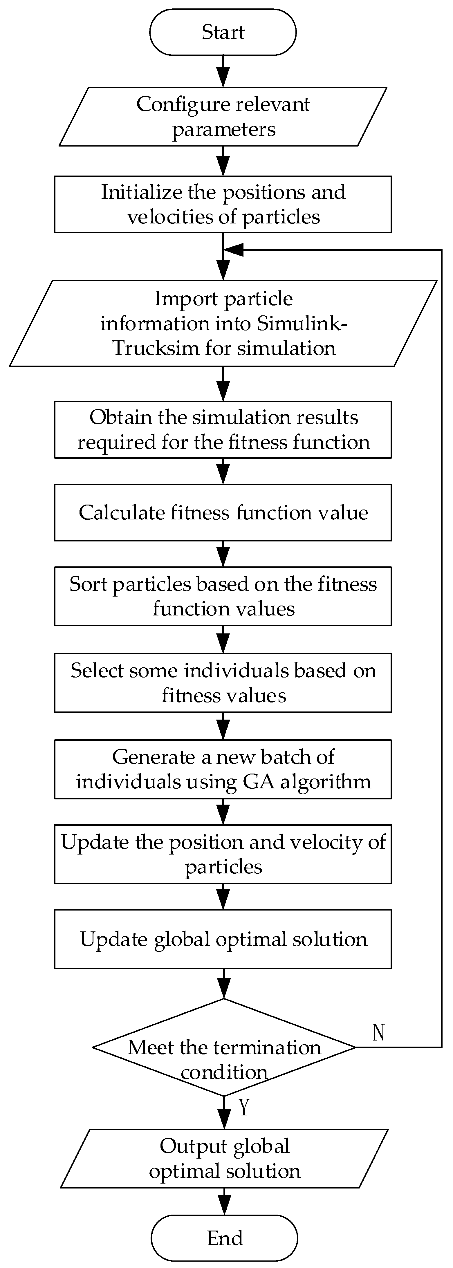
3.3. Optimization of Controller Parameters Based on GA-PSO Algorithm

The GA-PSO algorithm combines the advantages of the genetic algorithm (GA) [48] and Particle Swarm Optimization (PSO) [49] and demonstrates strong performance in solving complex optimization problems. The genetic algorithm (GA) explores the optimal solution space through selection, crossover, and mutation operations, while Particle Swarm Optimization (PSO) emulates the behavior of a particle swarm to identify the optimal solution. By combining these two algorithms, the GA-PSO algorithm achieves a balance between global and local searches, resulting in improved search efficiency, higher-quality optimization results, and more effective resolution of optimization problems.

The LQR uses a weight coefficient matrix to assign weights to control objectives, such as the states and inputs. The selection of weights greatly affects the control performance of the LQR path tracking controller. However, the selection of weight coefficient matrices is often based on experience, resulting in poor control effects. Similarly, in the design of FOSMC controllers, the selection of control law parameters significantly impacts their performance and robustness. Typically, the selection of control law parameters involves significant uncertainty due to relying on experience methods. To address these parameter selection challenges, this paper adopts the GA-PSO method to optimize the control law parameters of the LQR (Q and R) as well as FOSMC. Figure 5 shows the algorithm flow chart that applies GA-PSO to optimize the parameters of the LQR and FOSMC. The fitness function is a fundamental element of the GA-PSO algorithm. Considering the characteristics and operating conditions of distributed drive electric trucks, as well as the relationship between frequency and time domains, the fitness function was designed to incorporate the accuracy and stability of vehicle path tracking. It uses the sum of the integral time and absolute value (ITAE) of lateral error, heading error, center of mass sideslip angle error, and yaw rate error, as represented in Equation (36).

$$J=\min \left({\displaystyle {\int }_0^{T}t}\left|e_d(t)\right|\mathrm{d}t+{\displaystyle {\int }_0^{T}t}\left|e_{\phi }(t)\right|\mathrm{d}t+{\displaystyle {\int }_0^{T}t}\left|e_{\omega }(t)\right|\mathrm{d}t+{\displaystyle {\int }_0^{T}t}\left|e_{\beta }(t)\right|\mathrm{d}t\right)$$

(36)

For the GA-PSO algorithm, since it is mainly based on the PSO algorithm, each particle in the swarm is composed of its own position and velocity, which can be represented by Equation (37).

$$\left\{\begin{array}{l}{V}_j(t+1)=\eta V{(t)}_j+{\sigma }_1{r}_1\left(p_{\mathrm{best}\_\mathrm{j} }-P_j(t)\right)+{\sigma }_2{r}_2\left(g_{\mathrm{best} }-P_j(t)\right)\\ P_j(t+1)=P_j(t)+V_j(t+1)\end{array}\right.$$

(37)

where $V_j(t)$ and $P_j(t)$ are the velocity and position of the j-th particle in the t-th iteration, $p_{\mathrm{best}\_\mathrm{j} }$ is the personal optimal solution of the j-th particle, $g_{\mathrm{best} }$ is the current global optimal solution, ${\sigma }_1$ and ${\sigma }_2$ are learning factors, $r_1$ and $r_2$ are random numbers between [0, 1]; $\eta$ is the inertia factor.

Combining the fitness function and velocity-position updating formulas, the specific process of optimizing the controller parameters using GA-PSO is described below:

(1)

First, configure the relevant parameters. The specific configuration parameters are as follows: Particle Upper and Lower Limit Range; Population Size; Max Iterations; Mutation Probability; Crossover Probability; Inertia Weight of PSO; Cognitive Learning Factor of PSO; Social Learning Factor of PSO; Max Velocity of PSO.

(2)

Initialize the particle positions and velocities within the given value range.

(3)

Input the parameter information of each particle into the Simulink-TruckSim joint simulation program to obtain the values required for fitness function calculations.

(4)

Calculate the fitness function value for each particle and sort them based on the fitness function value.

(5)

Select a subset of particles with lower fitness function values and generate a new batch of individuals through GA cross-mutation operations.

(6)

Update the particle velocities and positions using the PSO velocity and position updating formulas, and simultaneously update the global best solution.

(7)

Determine whether the termination condition is met. If it is met, output the global best solution; otherwise, continue with Step (3) to Step (7) in a loop.

3.4. Design of Lower Layer Torque Distribution Controller

3.4.1. Longitudinal PID Speed Controller

The role of the longitudinal velocity controller is to calculate the total longitudinal driving force while simultaneously following the desired longitudinal vehicle speed. The longitudinal driver model employs a PID controller, as shown in Equation (38), for control. The total driving force $F_{t }$ of the vehicle is computed based on the deviation between the actual vehicle speed, $v_x$, and the desired vehicle speed, $v_d$.

$$F_{t }=K_p\left(v_d-v_x\right)+K_i{\displaystyle \int \left(v_d-v_x\right)}\mathrm{d}t+K_d\frac{\mathrm{d}\left(v_d-v_x\right)}{\mathrm{d}t}$$

(38)

where $K_p$, $K_i$, and $K_d$ are the proportional coefficient, integral coefficient, and differential coefficient of the PID controller, respectively.

3.4.2. Objective Function

Based on the additional lateral moment calculated by the intermediate stability controller and the longitudinal total driving force calculated by the longitudinal PID velocity controller, a reasonable torque distribution needs to be applied to the four wheels. Tire utilization refers to the ratio of the road adhesion on a single wheel to its maximum adhesion under the current operating condition. It mainly reflects the utilization of adhesion between the wheel and the road surface and also represents the stability margin of the vehicle [50]. The lower the tire utilization, the greater the stability margin and the higher the stability of the vehicle. Conversely, the higher the tire utilization, the lower the stability of the vehicle. Therefore, this paper establishes an objective function to minimize the tire utilization of the four wheels, in order to improve the driving stability of the vehicle.

$$J_{tire}=\min {\displaystyle \sum \frac{F_{xi}^2+F_{yi}^2}{{\mu }^2{F}_{zi}^2}},i=fl,fr,rl,rr$$

(39)

where $F_{xi}$ is the longitudinal force of the four wheels, $F_{yi}$ is the lateral force of the four wheels, and $F_{zi}$ is the vertical load of the four wheels.

Considering that there is a certain coupling relationship between tire lateral force and driving force, it is difficult to control the lateral force and it is relatively smaller compared to the driving force. Therefore, the influence of lateral force is not considered here, and the objective function is simplified to the form of Equation (40).

$$J_{tire}=\min {\displaystyle \sum \frac{F_{xi}^2}{{\mu }^2{F}_{zi}^2}},i=fl,fr,rl,rr$$

(40)

The relationship between wheel torque and tire longitudinal force can be expressed as Equation (41).

$$F_{xi}=\frac{T_i}{R}$$

(41)

Due to the assumption that the effective rolling radii of the four wheels are the same and remain constant, combined with Equations (40) and (41), the objective function can be written as Equation (42).

$$J_{tire}=\min {\displaystyle \sum \frac{T_i^2}{{\mu }^2{F}_{zi}^2}},i=fl,fr,rl,rr$$

(42)

3.4.3. Constraint Condition

When torque is distributed, each wheel should simultaneously satisfy the constraints of the additional lateral yaw moment and the overall driving force of the vehicle. The constraint equation is given by Equation (43).

$$\left\{\begin{array}{l}\left(F_{xfl}+F_{xfr}\right)\cos \delta +\left(F_{xrl}+F_{xrr}\right)=F_t\\ \frac{d_f}{2}\left(F_{xfr}-F_{xfl}\right)\cos \delta +\frac{d_r}{2}\left(F_{xrr}-F_{xrl}\right)=\Delta M_z\end{array}\right.$$

(43)

Under the conditions of meeting the above constraints, it is also necessary to consider the limitations of motor torque on motor performance and road adhesion conditions [51], thus establishing the inequality constraint of Equation (44).

$$\max \left(-\mu F_{zi}R,-T_{\max }\right)\le T_i\le \min \left(\mu F_{zi}R,T_{\max }\right),i=fl,fr,rl,rr$$

(44)

where $T_{\max }$ is the maximum torque output by the motor.

3.4.4. Optimization Problem Solving

Once the objective function and constraint conditions have been established, the torque distribution can be transformed into a multivariable function minimization problem, considering both equality and inequality constraints. Quadratic programming, an optimization method that utilizes quadratic optimization objectives and linear equality or inequality constraints, can address this problem. By optimizing the objective function, a more stable torque distribution scheme can be achieved, thereby enhancing the overall stability and controllability of the system. Consequently, the torque allocation problem addressed in this paper can be reformulated as a quadratic programming problem. By combining the determined objective function and constraints, the objective function can be expressed in the standard quadratic programming form as illustrated in Equation (45).

$$\begin{array}{l}\min J_{tire}=U^{T}WU\\ \mathrm{s}.\mathrm{t}. \left\{\begin{array}{l}HU=p\hfill \\ U_{\min }\le U\le U_{\max }\hfill \end{array}\right.\end{array}$$

(45)

where

$$U={\left[\begin{array}{cccc}{T}_{fl}& T_{fr}& T_{rl}& T_{rr}\end{array}\right]}^{\mathrm{T}}$$

(46)

$$W=\mathrm{diag}{\left[\begin{array}{cccc}\frac{1}{{\mu }^2{F}_{zfl}^2}& \frac{1}{{\mu }^2{F}_{zfr}^2}& \frac{1}{{\mu }^2{F}_{rl}^2}& \frac{1}{{\mu }^2{F}_{zrr}^2}\end{array}\right]}^{\mathrm{T}}$$

(47)

$$H=\left[\begin{array}{cccc}\cos \delta & \cos \delta & 1& 1\\ -\frac{d_f\cos \delta }{2}& \frac{d_f\cos \delta }{2}& -\frac{d_r}{2}& \frac{d_r}{2}\end{array}\right]$$

(48)

$$p=\left[\begin{array}{c}{F}_{t}R\\ \Delta M_{z}R\end{array}\right]$$

(49)

$$\left\{\begin{array}{l}{U}_{\min }=\max \left(-\mu F_{zi}R,-T_{\max }\right)\\ U_{\max }=\min \left(\mu F_{zi}R,T_{\max }\right)\end{array}\right.,i=fl,fr,rl,rr$$

(50)

There are several methods available to solve the quadratic programming problem. The two most commonly used methods are the interior point method and the active set method. The interior point method solves a sequence of constraint problems iteratively, gradually approaching the optimal solution. On the other hand, the active set method solves problems by identifying active and inactive constraints. Given that the optimal torque allocation problem discussed in this paper is a small-scale quadratic programming problem, it can be effectively solved using the “quadprog” function in MATLAB2020b. By solving this quadratic programming problem and obtaining the optimal solution, it can determine the torque allocated to each wheel, thereby effectively controlling the vehicle’s stability.

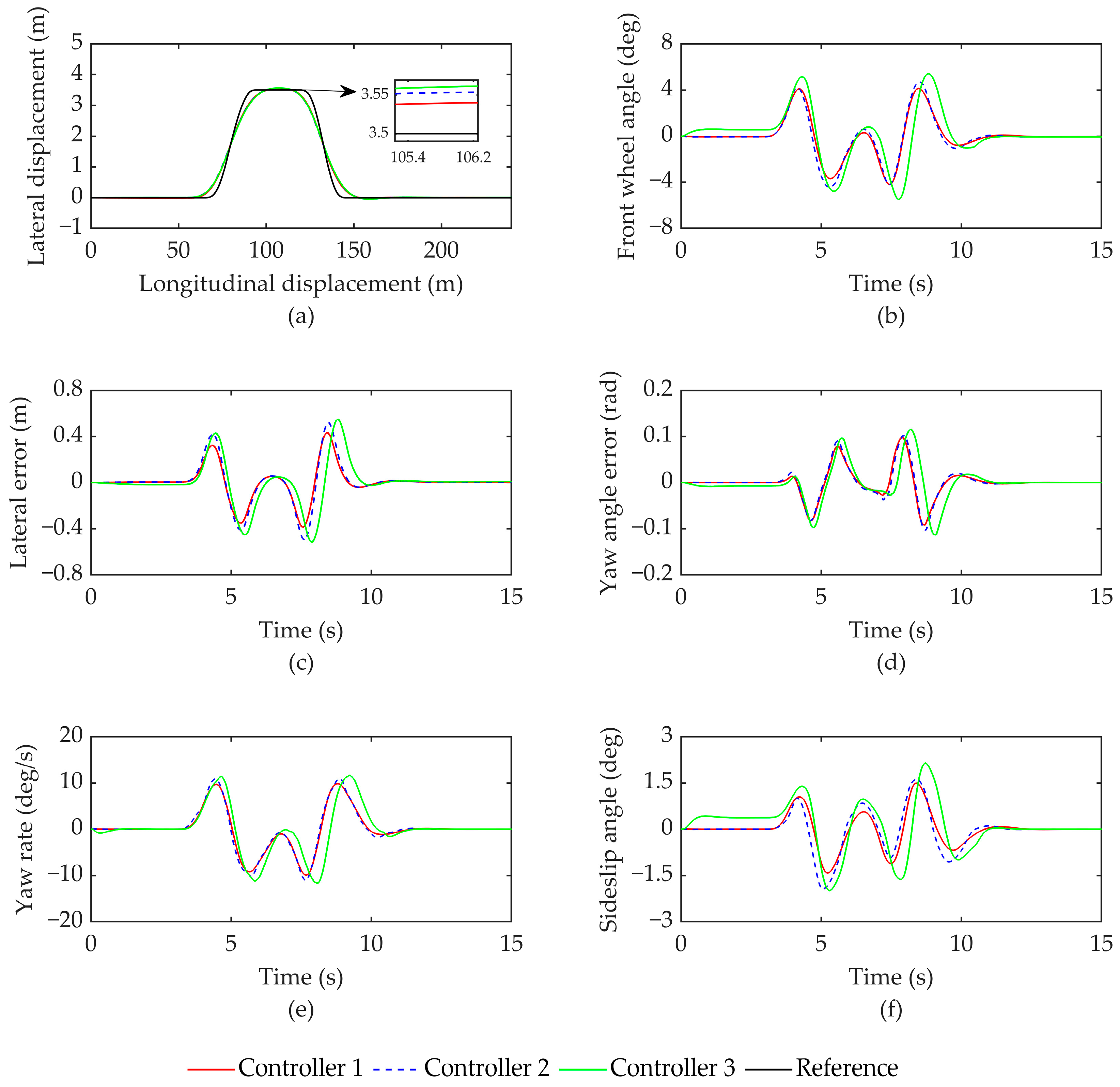
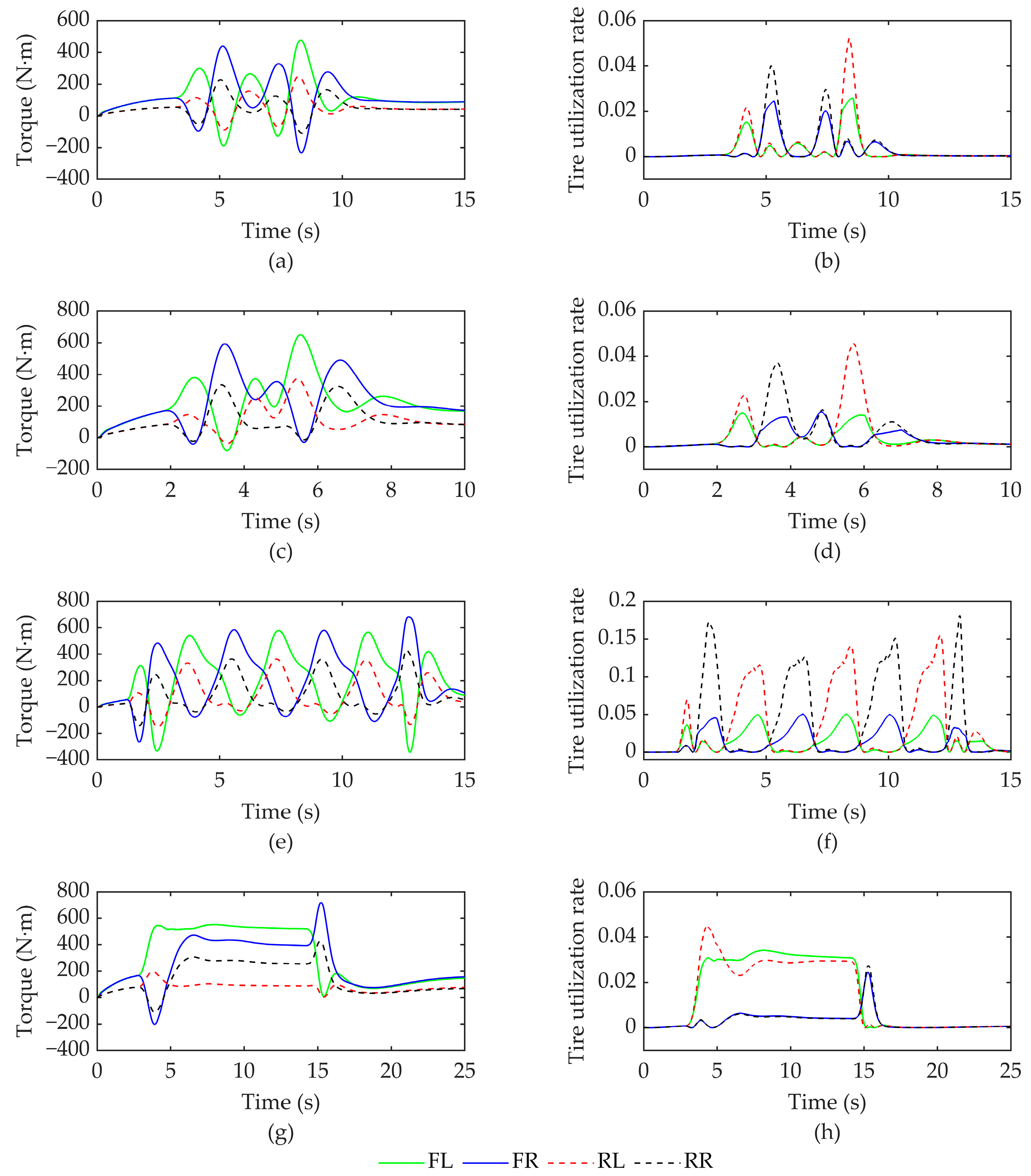
4. Simulation Analysis

In this section, the feasibility and effectiveness of the proposed strategy will be verified through simulation. The simulation was conducted on the MATLAB/Simulink-TruckSim joint simulation platform under the Intel Core i7-12700F CPU computer. The required vehicle-related parameters for the simulation are shown in

Table 1. Main parameters of vehicles.

Parameters	Units	Symbol	Value
Vehicle mass	Kg	$m$	5760
Distance from the center of mass to the front axis	mm	$a$	1250
Distance from the center of mass to the rear axis	mm	$b$	3750
Moment of inertia	Kg·m2	$I_z$	35,402.8
Front axle cornering stiffness	N/rad	$C_f$	−322,450
Rear axle cornering stiffness	N/rad	$C_r$	−330,030
Wheelbase of the front axle	mm	$d_f$	2030
Wheelbase of the rear axle	mm	$d_r$	1863
Height of the center of mass	mm	$h$	1175
Effective radius of wheel	mm	$R$	510
Maximum torque of vehicle drive motor	N·m	$T_i$	800

.

Four distinct simulation conditions were utilized for the purpose of comparing simulations, and the specific parameters associated with these conditions are outlined in

Table 2. Four simulation conditions parameters.

Working Condition	Reference Path	Tire–Road Friction Coefficient	Longitudinal Vehicle Speed
1	Double Lane Change	0.8	90 km/h
2	Double Lane Change	0.4	60 km/h
3	Serpentine	0.6	60 km/h
4	U-shaped	0.4	40 km/h

. Condition 1 involves tracking the motion along a double lane change path with an adhesion coefficient of 0.4 and a speed of 60 km/h. Condition 2 focuses on a road surface with an adhesion coefficient of 0.8, accompanied by a double lane change path and a speed of 90 km/h. Moving on to Condition 3, this condition considers a road surface with an adhesion coefficient of 0.6, with the tracking motion occurring along a snake-shaped path at a speed of 60 km/h. Lastly, Condition 4 entails a road surface with an adhesion coefficient of 0.4, with the tracking motion following a U-shaped path at a speed of 50 km/h. In order to demonstrate the superiority of the proposed strategy, three distinct controllers are established. Controller 1, named GA-PSO + LQR + FOSMC, is the control strategy put forth in this paper. Controller 2 comprises LQR + FOSMC, while Controller 3 consists of LQR + SMC. Subsequent charts represent Controller 1, Controller 2, and Controller 3. The relevant parameter values for Controller 1 are as follows: Q = diag [10.46,5.61,0.01,4.49], R = 0.01, ε = 0.001, and k = 26.6. Meanwhile, the empirical values for the relevant parameters in Controller 2 and Controller 3 are Q = diag [1,1,0.1,0.1], R = 1, ε = 0.1, and k = 50.

The simulation results for condition 1 are depicted in Figure 6, and the corresponding evaluation parameters are recorded in

Table 3. Evaluation parameters and their values related to condition 1.

Controller	Lateral Error (m)		Yaw Error (rad)		Yaw Rate (deg/s)		Sideslip Angle (deg)
	Max (abs)	RMS	Max (abs)	RMS	Max (abs)	RMS	Max (abs)	RMS
1	0.4353	0.1351	0.0978	0.0303	9.9031	4.1593	1.4905	0.5294
2	0.5224	0.1663	0.1033	0.0322	10.9972	4.4138	1.9316	0.6331
3	0.5518	0.1805	0.1161	0.0370	11.6401	4.8989	2.1444	0.8032

. Figure 6a shows that all three controllers effectively follow the reference path at a speed of 60 km/h, with only minor deviations observed at bends. This demonstrates good tracking performance. By analyzing the data presented in Figure 6c,d, along with Table 3, it can be concluded that controller 1 exhibits a maximum lateral error of 0.4353 m and a maximum heading error of 0.0978 rad. In comparison to controllers 2 and 3, the root mean square values of lateral error were reduced by 18.76% and 25.15%, respectively, while the root mean square values of heading error were reduced by 5.90% and 18.11%, respectively. Consequently, the vehicle’s tracking accuracy was significantly enhanced.

From Figure 6b, it can be observed that Controller 1 has the smallest steering angle for the front wheels, with a maximum value not exceeding 4 degrees. The angle fluctuation is smooth and continuous, which effectively enhances path tracking accuracy and vehicle stability. Combining the data in Table 3, Figure 6e,f, it can be inferred that the yaw rate and lateral deviation angle of the vehicle under the three controllers can be controlled within a certain range. However, the control effect of Controller 1 is superior. Compared to Controllers 2 and 3, the root mean square values of yaw rate decrease by 5.77% and 15.10%, respectively, while the root mean square values of lateral deviation angle decrease by 16.38% and 34.09%, respectively. This implies that Controller 1 has better control effectiveness in terms of vehicle stability, thereby enhancing the stability of vehicle driving.

In comparison to the low-speed- and low adhesion scenario of Condition 1, Condition 2 represents a high-speed- and high adhesion scenario. In this high-speed scenario, the requirement for vehicle stability is higher. Furthermore, maintaining path tracking accuracy is more challenging than at low speeds. The simulation results under Condition 2 are shown in Figure 7, and

Table 4. Evaluation parameters and their values related to condition 2.

Controller	Lateral Error (m)		Yaw Error (rad)		Yaw Rate (deg/s)		Sideslip Angle (deg)
	Max (abs)	RMS	Max (abs)	RMS	Max (abs)	RMS	Max (abs)	RMS
1	0.7211	0.2244	0.0996	0.0351	10.6126	5.0915	1.6560	0.7197
2	0.8282	0.2687	0.1126	0.0417	11.5930	5.7655	2.1197	0.8911
3	0.8903	0.3076	0.1167	0.0437	12.9965	6.1480	2.3285	1.0518

records the values of relevant evaluation parameters.

From Figure 7a,c,d, it is evident that even when the road condition is good, the tracking error of the vehicle significantly increases at a speed of 90 km/h compared to Condition 1. However, Controller 1 still manages to keep the lateral error and heading error within 0.7211 m and 0.0996 rad, respectively, demonstrating its effectiveness. Additionally, Controller 1 exhibits better path tracking accuracy at high speeds compared to Controller 2 and Controller 3, as evidenced by the reduction in the root mean square values of the lateral error and heading error by 16.49% and 27.05%, respectively. In Figure 7b, it can be observed that even under high-speed conditions, Controller 1 maintains the minimum front wheel angle and limits it to 4°. Furthermore, the combination of Figure 7e,f confirms that Controller 1 ensures excellent vehicle driving stability while also guaranteeing path tracking accuracy, thus validating the coordinated control strategy proposed in this study. Moreover, according to the data presented in Table 4, Controller 1 outperforms the other two controllers, exhibiting a decrease of 11.69% and 17.18% in yaw rate and root mean square value of center of mass sideslip angle, respectively, compared to Controller 2, and a decrease of 19.23% and 31.57%, respectively, compared to Controller 3.

The condition commonly employed to assess vehicles’ driving stability is the serpentine condition. Specifically, for this study, Condition 3 involves a serpentine path tracking motion carried out at low speed on medium adhesion road surfaces. The simulation results, presented in Figure 8, indicate that the relevant data have been documented in

Table 5. Evaluation parameters and their values related to condition 3.

Controller	Lateral Error (m)		Yaw Error (rad)		Yaw Rate (deg/s)		Sideslip Angle (deg)
	Max (abs)	RMS	Max (abs)	RMS	Max (abs)	RMS	Max (abs)	RMS
1	0.3791	0.1374	0.2251	0.0525	19.5200	12.0581	3.0144	1.2756
2	0.4340	0.1544	0.2349	0.0624	21.6897	13.1355	3.8459	1.4340
3	0.4561	0.1859	0.2954	0.0660	23.7043	13.8848	4.0700	2.1310

. Upon examining Figure 8a,c,d, it becomes evident that although all three controllers are capable of effectively tracking the desired path, Controller 3 exhibits a significantly larger tracking error when compared to Controller 1 and Controller 2. Moreover, according to the data provided in Table 5, Controller 1’s root mean square values for lateral error and heading error have decreased by 11.01%, 26.09%, 15.87%, and 20.45% in comparison to Controllers 2 and 3, respectively. Consequently, the tracking accuracy has noticeably improved. From Figure 8b, it can be seen that under the serpentine working condition, the number of turns of the vehicle significantly increases, and the driving stability control of the vehicle is more important. Compared to controller 1, the front wheel angle is smaller and converges faster. Observing Figure 8e,f, it can be seen that the fluctuations in the yaw rate and center of mass sideslip angle of Controller 3 are more significant. This is due to the existence of chattering problems in traditional SMC controllers. With Controller 1 and Controller 2 using FOSMC, chattering is well suppressed. Controller 1 has been optimized by 8.20% and 13.16% in terms of yaw rate compared to controllers 2 and 3, respectively; in terms of centroid sideslip angle, 11.05% and 40.14% were optimized, respectively, indicating that the control strategy proposed in this paper greatly improves the driving stability of the vehicle.

The simulation results under condition 4 are presented in Figure 9, with the relevant data recorded in

Table 6. Evaluation parameters and their values related to condition 4.

Controller	Lateral Error (m)		Yaw Error (rad)		Yaw Rate (deg/s)		Sideslip Angle (deg)
	Max (abs)	RMS	Max (abs)	RMS	Max (abs)	RMS	Max (abs)	RMS
1	0.2329	0.1223	0.0919	0.0584	11.5801	8.4870	1.8646	1.3744
2	0.3092	0.1610	0.1124	0.0705	12.8955	9.3652	2.3421	1.4453
3	0.3309	0.1825	0.1460	0.0954	13.3003	9.7098	2.6273	1.8877

. The U-shaped working condition, commonly encountered by trucks, involves significant curvature changes and imposes high requirements for vehicle tracking and stability control. In Condition 4, a U-turn is performed on a road surface with a coefficient of adhesion of 0.4 at a speed of 50 km/h. Figure 9a clearly shows that all three controllers effectively track the reference path. The analysis of the data from Figure 9c and Table 6 demonstrates that all three controllers maintain a lateral error within 0.35 m and a heading error within 0.15 rad, indicating excellent tracking performance. Notably, controller 1 exhibits significantly smaller tracking errors compared to the other two controllers, with reductions of 23.31% and 32.99% in lateral error and 17.16% and 38.78% in heading error, illustrating its higher tracking accuracy.

Figure 9b reveals that controller 1 exhibits the smallest front wheel angle and smoother transitions during curve entry and exit, resulting in significant improvements in the vehicle’s operational stability. A comparison between Figure 9e,f clearly demonstrates that controller 1 achieves a considerably enhanced vehicle stability control effect, outperforming controllers 2 and 3. Notably, this improvement in stability is evident in the optimization of the root mean square value, with the yaw rate being optimized by 9.38% and 12.59%, respectively, and the center of mass sideslip angle experiencing optimizations of 4.91% and 27.19%, respectively. When compared to controllers 2 and 3, controller 1, implementing the control strategy proposed in this paper, not only ensures high tracking accuracy but also enhances vehicle stability.

Figure 10 illustrates the torque distribution and tire utilization of controller 1 across four different operating conditions. Specifically, Figure 10a,c,e,g display the torque distribution among the four wheels during condition 1, condition 2, condition 3, and condition 4, respectively. The figures indicate that the torque applied to the front axle wheels is consistently higher than that applied to the rear axle wheels under these conditions. This result is achieved by dynamically adjusting the torque optimization distribution controller based on the wheel load, enabling improved stability. Notably, the torque allocation control strategy ensures that the front wheel consistently receives a greater torque than the rear wheel, optimizing the utilization of the carrying tire’s adhesion and enhancing the stability of the smaller carrying wheel. Conversely, Figure 10b,d,f,h illustrate that this paper’s optimized torque distribution strategy effectively maintains the tire utilization rate for all four wheels within a 0.06 range during conditions 1, 2, and 4. However, due to continuous steering, condition 3 exhibits a higher tire utilization rate compared to the other conditions. Yet, the maximum tire utilization rate remains below 0.2, indicating sufficient vehicle stability margin. Moreover, the optimized torque distribution strategy not only facilitates the vehicle’s ability to generate the required lateral force for turning but also ensures stable driving. These findings validate the effectiveness of the proposed torque distribution strategy in this study.

5. Conclusions

This article discusses the coordinated control problem of path tracking and yaw stability control for four-wheel independent drive electric trucks. A hierarchical control framework has been designed to address this issue. In the upper controller design, an LQR path tracking controller was established, and steady-state error was eliminated through feedforward control to achieve precise steering control. The middle controller utilizes the FOSMC yaw torque controller to calculate additional yaw torque based on the steering angle input from the upper layer. Additionally, the weight coefficients of LQR and the sliding mode parameters of FOSMC are optimized using GA-PSO. The lower layer torque distribution controller employs the quadratic programming method to resolve the tire utilization objective function in real time. This allows for optimal torque distribution, thereby enhancing the vehicle’s stability control margin. A joint simulation of four different operating conditions was performed using MATLAB/Simulink-TruckSim. The results indicate that, in comparison to the other two controllers, the GA-PSO + LQR + FOSMC controller proposed in this study achieves smaller tracking deviation. Specifically, the tracking performance of the proposed control scheme has been improved by 15.54% and 23.17%, respectively, under the average tracking error of the four different operating conditions. Moreover, the vehicle’s driving stability has been improved by 10.83% and 23.88%, respectively, thereby enhancing the vehicle’s yaw stability and driving safety. The optimal allocation strategy based on the quadratic programming method ensures the tire utilization rate remains within 0.2, significantly boosting the stability margin of the vehicle. In summary, the proposed coordinated control strategy effectively enhances the tracking performance of four-wheel independent drive electric trucks under various complex driving conditions, while also increasing the vehicle’s driving stability. Therefore, the proposed control scheme can serve as a theoretical reference for the development of path tracking and stability control for four-wheel independent drive electric trucks.

In future work, the control strategy will be further applied to actual vehicles for experimental verification. These experiments will be conducted under stricter and more complex conditions to validate the performance of the proposed strategy.

References

1. Nascimento, A.M.; Vismari, L.F.; Molina, C.B.S.T.; Cugnasca, P.S.; Camargo, J.B.; Almeida, J.R.; de Inam, R.; Fersman, E.; Marquezini, M.V.; Hata, A.Y. A Systematic Literature Review About the Impact of Artificial Intelligence on Autonomous Vehicle Safety. IEEE Trans. Intell. Transp. Syst. 2020, 21, 4928–4946. [Google Scholar] [CrossRef]
2. Yang, H.; Zheng, C.; Zhao, Y.; Wu, Z. Integrating the Intelligent Driver Model With the Action Point Paradigm to Enhance the Performance of Autonomous Driving. IEEE Access 2020, 8, 106284–106295. [Google Scholar] [CrossRef]
3. Cao, M.; Li, V.O.K.; Shuai, Q. DeepGAL: Intelligent Vehicle Control for Traffic Congestion Alleviation at Intersections. IEEE Trans. Intell. Transp. Syst. 2023, 24, 6836–6848. [Google Scholar] [CrossRef]
4. Guo, N.; Zhang, X.; Zou, Y.; Lenzo, B.; Zhang, T. A Computationally Efficient Path-Following Control Strategy of Autonomous Electric Vehicles With Yaw Motion Stabilization. IEEE Trans. Transp. Electrif. 2020, 6, 728–739. [Google Scholar] [CrossRef]
5. An, X.; Cai, B.; Shangguan, W. Research on Industry Development and Key Technologies of Vehicle Infrastructure Cooperative Autonomous Driving. In Proceedings of the Sixth International Conference on Traffic Engineering and Transportation System (ICTETS 2022), Guangzhou, China, 16 February 2023; SPIE: Bellingham, DC, USA, 2023; Volume 12591, pp. 669–677. [Google Scholar]
6. Huang, Y.; Ding, H.; Zhang, Y.; Wang, H.; Cao, D.; Xu, N.; Hu, C. A Motion Planning and Tracking Framework for Autonomous Vehicles Based on Artificial Potential Field Elaborated Resistance Network Approach. IEEE Trans. Ind. Electron. 2020, 67, 1376–1386. [Google Scholar] [CrossRef]
7. Yao, J.; Ge, Z. Path-Tracking Control Strategy of Unmanned Vehicle Based on DDPG Algorithm. Sensors 2022, 22, 7881. [Google Scholar] [CrossRef]
8. Chen, J.; Shuai, Z.; Zhang, H.; Zhao, W. Path Following Control of Autonomous Four-Wheel-Independent-Drive Electric Vehicles via Second-Order Sliding Mode and Nonlinear Disturbance Observer Techniques. IEEE Trans. Ind. Electron. 2021, 68, 2460–2469. [Google Scholar] [CrossRef]
9. Liang, Y.; Li, Y.; Khajepour, A.; Zheng, L. Holistic Adaptive Multi-Model Predictive Control for the Path Following of 4WID Autonomous Vehicles. IEEE Trans. Veh. Technol. 2021, 70, 69–81. [Google Scholar] [CrossRef]
10. Deng, X.; Sun, H.; Lu, Z.; Cheng, Z.; An, Y.; Chen, H. Research on Dynamic Analysis and Experimental Study of the Distributed Drive Electric Tractor. Agriculture 2023, 13, 40. [Google Scholar] [CrossRef]
11. Tian, J.; Wang, Q.; Ding, J.; Wang, Y.; Ma, Z. Integrated Control With DYC and DSS for 4WID Electric Vehicles. IEEE Access 2019, 7, 124077–124086. [Google Scholar] [CrossRef]
12. Wang, W.; Ma, T.; Yang, C.; Zhang, Y.; Li, Y.; Qie, T. A Path Following Lateral Control Scheme for Four-Wheel Independent Drive Autonomous Vehicle Using Sliding Mode Prediction Control. IEEE Trans. Transp. Electrif. 2022, 8, 3192–3207. [Google Scholar] [CrossRef]
13. Rupp, A.; Stolz, M. Survey on Control Schemes for Automated Driving on Highways. In Automated Driving: Safer and More Efficient Future Driving; Watzenig, D., Horn, M., Eds.; Springer International Publishing: Cham, Switzerland, 2017; pp. 43–69. ISBN 978-3-319-31895-0. [Google Scholar]
14. Cheng, Z.; Lu, Z. Research on Load Disturbance Based Variable Speed PID Control and a Novel Denoising Method Based Effect Evaluation of HST for Agricultural Machinery. Agriculture 2021, 11, 960. [Google Scholar] [CrossRef]
15. Tan, Y.; Wen, B.; Jiao, C.; Su, X.; Xue, F. Trajectory Tracking Control of Differential Steering Mobile Robot Based on Fuzzy Logic under Time Constraints. In Proceedings of the 2021 33rd Chinese Control and Decision Conference (CCDC), Kunming, China, 22–24 May 2021; pp. 5225–5229. [Google Scholar]
16. Wu, Y.; Wang, L.; Zhang, J.; Li, F. Path Following Control of Autonomous Ground Vehicle Based on Nonsingular Terminal Sliding Mode and Active Disturbance Rejection Control. IEEE Trans. Veh. Technol. 2019, 68, 6379–6390. [Google Scholar] [CrossRef]
17. Tian, J.; Yang, M. Research on Trajectory Tracking and Body Attitude Control of Autonomous Ground Vehicle Based on Differential Steering. PLoS ONE 2023, 18, e0273255. [Google Scholar] [CrossRef] [PubMed]
18. Nguyen, A.-T.; Sentouh, C.; Zhang, H.; Popieul, J.-C. Fuzzy Static Output Feedback Control for Path Following of Autonomous Vehicles with Transient Performance Improvements. IEEE Trans. Intell. Transp. Syst. 2020, 21, 3069–3079. [Google Scholar] [CrossRef]
19. Li, B. Unbalanced Vibration Control of Active Magnetic Bearing Using an Active Disturbance Rejection Notch Decoupling Technique. J. Vib. Control 2023, 107754632311564. [Google Scholar] [CrossRef]
20. Wang, Y.; Wang, J.; Yang, J.; Du, R.; Hai, Z.; Deng, H. Research on Path Tracking Control of Unmanned Vehicle. J. Phys. Conf. Ser. 2023, 2480, 012002. [Google Scholar] [CrossRef]
21. Saleem, O.; Iqbal, J. Fuzzy-Immune-Regulated Adaptive Degree-of-Stability LQR for a Self-Balancing Robotic Mechanism: Design and HIL Realization. IEEE Robot. Autom. Lett. 2023, 8, 4577–4584. [Google Scholar] [CrossRef]
22. Zhao, C.; Zhang, C.; Guo, F.; Shao, Y. Research on Path Following Control Method of Agricultural Machinery Autonomous Navigation through LQR-Feed Forward Control. In Proceedings of the 2021 IEEE International Conference on Data Science and Computer Application (ICDSCA), Dalian, China, 29–31 October 2021; pp. 228–233. [Google Scholar]
23. Li, H.; Li, P.; Yang, L.; Zou, J.; Li, Q. Safety Research on Stabilization of Autonomous Vehicles Based on Improved-LQR Control. AIP Adv. 2022, 12, 015313. [Google Scholar] [CrossRef]
24. Xu, S.; Peng, H. Design, Analysis, and Experiments of Preview Path Tracking Control for Autonomous Vehicles. IEEE Trans. Intell. Transp. Syst. 2020, 21, 48–58. [Google Scholar] [CrossRef]
25. Kapania, N.R.; Gerdes, J.C. Design of a Feedback-Feedforward Steering Controller for Accurate Path Tracking and Stability at the Limits of Handling. Veh. Syst. Dyn. 2015, 53, 1687–1704. [Google Scholar] [CrossRef]
26. Ni, J.; Wang, Y.; Li, H.; Du, H. Path Tracking Motion Control Method of Tracked Robot Based on Improved LQR Control. In Proceedings of the 2022 41st Chinese Control Conference (CCC), Hefei, China, 25–27 July 2022; pp. 2888–2893. [Google Scholar]
27. Wang, Z.; Sun, K.; Ma, S.; Sun, L.; Gao, W.; Dong, Z. Improved Linear Quadratic Regulator Lateral Path Tracking Approach Based on a Real-Time Updated Algorithm with Fuzzy Control and Cosine Similarity for Autonomous Vehicles. Electronics 2022, 11, 3703. [Google Scholar] [CrossRef]
28. Lu, A.; Lu, Z.; Li, R.; Tian, G. Adaptive LQR Path Tracking Control for 4WS Electric Vehicles Based on Genetic Algorithm. In Proceedings of the 2022 6th CAA International Conference on Vehicular Control and Intelligence (CVCI), Nanjing, China, 28–30 October 2022; pp. 1–6. [Google Scholar]
29. Lei, T.; Gu, X.; Zhang, K.; Li, X.; Wang, J. PSO-Based Variable Parameter Linear Quadratic Regulator for Articulated Vehicles Snaking Oscillation Yaw Motion Control. Actuators 2022, 11, 337. [Google Scholar] [CrossRef]
30. Hashemi, E.; Jalali, M.; Khajepour, A.; Kasaiezadeh, A.; Chen, S. Vehicle Stability Control: Model Predictive Approach and Combined-Slip Effect. IEEEASME Trans. Mechatron. 2020, 25, 2789–2800. [Google Scholar] [CrossRef]
31. Liang, Y.; Li, Y.; Yu, Y.; Zheng, L. Integrated Lateral Control for 4WID/4WIS Vehicle in High-Speed Condition Considering the Magnitude of Steering. Veh. Syst. Dyn. 2020, 58, 1711–1735. [Google Scholar] [CrossRef]
32. Lin, C.; Liang, S.; Gong, X.; Wang, B. Coordinated Yaw Stability Control for Extreme Path Tracking of 4WIDEVs Based on Predictive Control. Proc. Inst. Mech. Eng. Part J. Automob. Eng. 2023, 237, 1929–1946. [Google Scholar] [CrossRef]
33. Chatzikomis, C.; Sorniotti, A.; Gruber, P.; Zanchetta, M.; Willans, D.; Balcombe, B. Comparison of Path Tracking and Torque-Vectoring Controllers for Autonomous Electric Vehicles. IEEE Trans. Intell. Veh. 2018, 3, 559–570. [Google Scholar] [CrossRef]
34. Zhang, Z.; Zheng, L.; Li, Y.; Li, S.; Liang, Y. Cooperative Strategy of Trajectory Tracking and Stability Control for 4WID Autonomous Vehicles Under Extreme Conditions. IEEE Trans. Veh. Technol. 2023, 72, 3105–3118. [Google Scholar] [CrossRef]
35. Hu, C.; Wang, R.; Yan, F.; Chen, N. Output Constraint Control on Path Following of Four-Wheel Independently Actuated Autonomous Ground Vehicles. IEEE Trans. Veh. Technol. 2016, 65, 4033–4043. [Google Scholar] [CrossRef]
36. Zou, Y.; Guo, N.; Zhang, X. An Integrated Control Strategy of Path Following and Lateral Motion Stabilization for Autonomous Distributed Drive Electric Vehicles. Proc. Inst. Mech. Eng. Part J. Automob. Eng. 2021, 235, 1164–1179. [Google Scholar] [CrossRef]
37. Xie, J.; Xu, X.; Wang, F.; Tang, Z.; Chen, L. Coordinated Control Based Path Following of Distributed Drive Autonomous Electric Vehicles with Yaw-Moment Control. Control Eng. Pract. 2021, 106, 104659. [Google Scholar] [CrossRef]
38. Sun, H.; Li, J.; Wang, R.; Yang, K. Attitude Control of the Quadrotor UAV with Mismatched Disturbances Based on the Fractional-Order Sliding Mode and Backstepping Control Subject to Actuator Faults. Fractal Fract. 2023, 7, 227. [Google Scholar] [CrossRef]
39. Chan, J.C.L.; Lee, T.H. Sliding Mode Observer-Based Fault-Tolerant Secondary Control of Microgrids. Electronics 2020, 9, 1417. [Google Scholar] [CrossRef]
40. Gudey, S.K.; Malla, M.; Jasthi, K.; Gampa, S.R. Direct Torque Control of an Induction Motor Using Fractional-Order Sliding Mode Control Technique for Quick Response and Reduced Torque Ripple. World Electr. Veh. J. 2023, 14, 137. [Google Scholar] [CrossRef]
41. Talebi, J.; Ganjefar, S. Fractional Order Sliding Mode Controller Design for Large Scale Variable Speed Wind Turbine for Power Optimization. Environ. Prog. Sustain. Energy 2018, 37, 2124–2131. [Google Scholar] [CrossRef]
42. Al-Dhaifallah, M.; Al-Qahtani, F.M.; Elferik, S.; Saif, A.-W.A. Quadrotor Robust Fractional-Order Sliding Mode Control in Unmanned Aerial Vehicles for Eliminating External Disturbances. Aerospace 2023, 10, 665. [Google Scholar] [CrossRef]
43. Rajamani, R. Vehicle Dynamics and Control; Springer Science & Business Media: Berlin/Heidelberg, Germany, 2011; ISBN 978-1-4614-1432-2. [Google Scholar]
44. Tong, Y.; Jing, H.; Kuang, B.; Wang, G.; Liu, F.; Yang, Z. Trajectory Tracking Control for Four-Wheel Independently Driven Electric Vehicle Based on Model Predictive Control and Sliding Model Control. In Proceedings of the 2021 5th CAA International Conference on Vehicular Control and Intelligence (CVCI), Tianjin, China, 29–31 October 2021; pp. 1–5. [Google Scholar]
45. Li, S.; Wang, X.; Cui, G.; Lu, X.; Zhang, B. Yaw and Lateral Stability Control Based on Predicted Trend of Stable State of the Vehicle. Veh. Syst. Dyn. 2023, 61, 111–127. [Google Scholar] [CrossRef]
46. Hou, Y.; Xu, X. High-Speed Lateral Stability and Trajectory Tracking Performance for a Tractor-Semitrailer with Active Trailer Steering. PLoS ONE 2022, 17, e0277358. [Google Scholar] [CrossRef]
47. Afifa, R.; Ali, S.; Pervaiz, M.; Iqbal, J. Adaptive Backstepping Integral Sliding Mode Control of a MIMO Separately Excited DC Motor. Robotics 2023, 12, 105. [Google Scholar] [CrossRef]
48. Cheng, Z.; Chen, Y.; Li, W.; Liu, J.; Li, L.; Zhou, P.; Chang, W.; Lu, Z. Full Factorial Simulation Test Analysis and I-GA Based Piecewise Model Comparison for Efficiency Characteristics of Hydro Mechanical CVT. Machines 2022, 10, 358. [Google Scholar] [CrossRef]
49. Li, Y.; Ma, Z.; Zheng, M.; Li, D.; Lu, Z.; Xu, B. Performance Analysis and Optimization of a High-Temperature PEMFC Vehicle Based on Particle Swarm Optimization Algorithm. Membranes 2021, 11, 691. [Google Scholar] [CrossRef] [PubMed]
50. Li, Q.; Zhang, J.; Li, L.; Wang, X.; Zhang, B.; Ping, X. Coordination Control of Maneuverability and Stability for Four-Wheel-Independent-Drive EV Considering Tire Sideslip. IEEE Trans. Transp. Electrif. 2022, 8, 3111–3126. [Google Scholar] [CrossRef]
51. Mehmood, Y.; Aslam, J.; Ullah, N.; Alsheikhy, A.A.; Din, E.U.; Iqbal, J. Robust Fuzzy Sliding Mode Controller for a Skid-Steered Vehicle Subjected to Friction Variations. PLoS ONE 2021, 16, e0258909. [Google Scholar] [CrossRef] [PubMed]
Figure 1. 2DOF vehicle dynamics model.
Processes 11 02473 g001
Figure 2. 7DOF vehicle dynamics model.
Processes 11 02473 g002
Figure 3. Layered control system framework.
Processes 11 02473 g003
Figure 4. Path tracking error model.
Processes 11 02473 g004
Figure 5. GA-PSO algorithm parameter optimization flowchart.
Processes 11 02473 g005
Figure 6. Comparison of simulation results under condition 1: (a) vehicle trajectory; (b) front wheel angle; (c) lateral error; (d) yaw angle error; (e) yaw rate; (f) sideslip angle.
Processes 11 02473 g006
Figure 7. Comparison of simulation results under condition 2: (a) vehicle trajectory; (b) front wheel angle; (c) lateral error; (d) yaw angle error; (e) yaw rate; (f) sideslip angle.
Processes 11 02473 g007
Figure 8. Comparison of simulation results under condition 3: (a) vehicle trajectory; (b) front wheel angle; (c) lateral error; (d) yaw angle error; (e) yaw rate; (f) sideslip angle.
Processes 11 02473 g008
Figure 9. Comparison of simulation results under condition 4: (a) vehicle trajectory; (b) front wheel angle; (c) lateral error; (d) yaw angle error; (e) yaw rate; (f) sideslip angle.
Processes 11 02473 g009
Figure 10. Simulation results of torque distribution and tire utilization under four operating conditions (Controller 1). (a) Torque distribution under condition 1; (b) condition 1 tire utilization rate; (c) torque distribution under condition 2; (d) condition 2 tire utilization; (e) torque distribution under condition 3; (f) condition 3 tire utilization; (g) torque distribution under condition 4; (h) condition 4 tire utilization.
Processes 11 02473 g010