Bearing Fault Diagnosis Based on ICEEMDAN Deep Learning Network

Abstract

Bearing fault diagnosis has evolved from machine learning to deep learning, addressing the issues of performance degradation in deep learning networks and the potential loss of key feature information. This paper proposes a fault diagnosis method for rolling bearing faults based on ICEEMDAN combined with the Hilbert transform (ICEEMDAN-Hilbert) and a residual network (ResNet). Firstly, the collected fault vibration signals are classified as fault samples and randomly sampled with a fixed length. The IMF components obtained by decomposing the bearing fault vibration signals using ICEEMDAN are able to maximize the restoration of fault vibrations. Then, the IMF components are transformed from one-dimensional time-domain signals to two-dimensional time-frequency domain images using Hilbert transformation. The RGB color images can be directly used in deep learning models without the need for manual labeling of a large amount of data, thereby avoiding the loss of key feature information. The ResNet network incorporates the attention mechanism (CBAM) structure for the precise extraction of fault features, enabling a more detailed classification of fault features. Additionally, the residual network effectively addresses the problem of performance degradation in multi-layer network models. Finally, transfer learning is applied in the deep learning network by freezing the training layer parameters and training the fully connected layer. This effectively solves the problem of insufficient data in real operating conditions, which hinders deep training of the model, while also reducing the training time. By combining the ResNet network with the convolutional block attention module (CBAM) structure, the model completes the recognition and training of time-frequency images for rolling bearing faults. The results demonstrate that the ResNet with CBAM model has strong fault feature extraction capabilities, achieving higher accuracy, 7–12% higher than other conventional network models, and exhibiting superior diagnostic performance compared to other deep learning models.

1. Introduction

Rolling bearings are widely used in mechanical equipment and play a crucial role in the rotation of machinery [1]. Many rolling bearings operate under long-term high loads and in complex environments, making them susceptible to adverse working conditions and improper usage, which can lead to a shortened service life. Rapid detection of bearing faults can significantly reduce production risks, improve maintenance efficiency, and enhance the safety and reliability of production machinery. The extraction of characteristic information from the vibration signals of rolling bearings is employed in industrial fault diagnosis to reduce costs and prevent accidents caused by bearing failures. When bearings experience operational faults, complex interference signals, including modulated signals and impulse signals, can pose challenges in extracting characteristic frequencies of faults. Therefore, to eliminate interference signals, the accurate identification of the fault signal is the key factor in bearing fault signal diagnosis; thus, it becomes more important to extract fault features.

Currently, there are various methods for the treatment of bearing fault characteristics; the empirical mode decomposition (EMD) technique can decompose signals into different scale intrinsic mode function (IMF) components, making it suitable for non-stationary signals. However, due to the issue of mode mixing, the decomposition results are not satisfactory [2]. Torres et al. [3] proposed the complete ensemble empirical mode decomposition with adaptive noise (CEEMDAN) method, which introduces adaptive white noise to enhance the independence between modes, thereby extracting two originally inseparable modes. This method effectively solves the mode-mixing problem, reduces the residual noise in reconstructed signals, and decreases the number of siftings required. Colominas et al. [4] proposed an improved method called improved complete ensemble empirical mode decomposition with adaptive noise (ICEEMDAN), which addresses the deficiencies in the adaptive decomposition of EMD and significantly reduces the residual components in the IMF, resulting in better reconstruction results and a further improvement in the mode-mixing problem [5]. In the fault diagnosis of actual engineering machinery, especially in the early occurrence of bearing fault, the fault signal is weak, and with the interference of noise, the cycle characteristics of the pulse signal are difficult to extract from the composite signal; thus, the single ICEEMDAN method cannot accurately show the bearing fault diagnosis. Because of the excellent implied deep learning model feature extraction and data processing ability, it also has a wide application in the field of engineering.

Qiu et al. [6] aimed to achieve the diversity and variability of practical fault diagnosis distributions. They used feature extraction methods such as time-domain analysis, frequency-domain analysis, and wavelet packet decomposition to obtain relevant indicators. Subsequently, they employed convolutional neural networks (CNNs) for intelligent fault diagnosis of gearboxes. Sun et al. [7] focused on improving the accuracy of fault diagnosis for rolling bearings in the target area, considering the diversity of real fault diagnosis distributions. They proposed a sparse additive noise elimination autoencoder algorithm with adaptive solution regions. Che et al. [8] proposed a region-adaptive deep belief network suitable for rolling bearing fault diagnosis, addressing the issue of the inability to collect rolling bearing sample labels in various working environments. These bearings need manual tagging to extract fault features; even for smaller sample tag numbers, the required sample size is large, and one cannot have a lot of samples in real engineering, but since it is insensitive to noise, the characteristics of the fault signal can be extracted accurately.

He et al. [9] proposed a method for improving the accurate identification of different types of bearing faults under different operating conditions. They applied a short-time Fourier transform (STFT) to preprocess the signals obtained from sensors and then constructed a deep learning structure using a simple spectrogram matrix for bearing fault diagnosis. Xu et al. [10] aimed to address the problem of overlooked features during fault feature extraction. They proposed a hybrid model combining a CNN and a deep forest algorithm. The vibration signals of bearings were transformed into time-frequency images using continuous wavelet transform (CWT), and the CNN was used to extract features, which were then input into the deep forest classifier for fault type identification. The appeal method uses a deep learning model; in bearing fault diagnosis, the accuracy has a degree of improvement, but there is no deep excavation of weak fault signal characteristics, meaning that periodic weak characteristic signals are ignored.

In machine learning, a large amount of labeled data is typically required for training. However, in practical work environments, it is often not feasible to label a large quantity of fault vibration data. Manually dividing features during feature extraction can lead to the oversight of subtle feature signals, resulting in misdiagnosis in fault detection. In the field of deep learning, network models can automatically extract and recognize features, avoiding the influence of manual feature selection during feature signal extraction. However, as the depth of deep learning models increases, issues such as overfitting and declining performance may arise. In different operating conditions encountered in actual production, the accuracy of fault diagnosis for rolling bearings can be easily affected by strong noise interference from the external environment, thus impacting the accuracy of diagnosis and recognition.

This paper proposes a bearing diagnosis method based on ICEEMDAN-Hilbert and a residual network (ResNet-CBAM) for rolling bearing fault diagnosis. Firstly, ICEEMDAN is used to decompose the fault vibration signals of the bearings, allowing the IMF components obtained from the decomposition to maximize the restoration of the fault vibration signals and avoid the occurrence of false modal signals. The Hilbert transform is then applied to convert the decomposed IMF components from one-dimensional time-domain signals into two-dimensional time-frequency domain images, which can be directly applied to deep learning models in computer vision without the need for manual labeling of a large amount of data. By randomly sampling the original vibration signals with a fixed length, a complete set of randomly sampled fault samples is created, facilitating the accurate extraction of fault features by the attention mechanism structure in the network model and enabling a more detailed classification of fault features. Finally, transfer learning is employed in the deep learning network by freezing the training layer parameters and training the fully connected layers, effectively addressing the lack of a large amount of data in real-world operating conditions, which would otherwise hinder deep training of the model, while also reducing the training time. The combination of ResNet and CBAM structures is used for the recognition and training of time-frequency images of rolling bearing faults. The results demonstrate that the ResNet-CBAM diagnosis model has strong fault feature extraction capabilities and outperforms other deep learning models in diagnostic performance.

2. The Methodology

2.1. The Fundamental Theory of ICEEMDAN

A new method for fault diagnosis of rolling bearings is based on the combination of ICEEMDAN (improved complete ensemble empirical mode decomposition with adaptive noise) and the Hilbert transform, resulting in an improved ICEEMDAN-Hilbert transform. Subsequently, the transformed Hilbert envelope is combined with an improved residual network.

To address the issues observed in methods like EEMD, Torres et al. [3] proposed complete ensemble empirical mode decomposition with adaptive noise (CEEMDAN) with adaptive white noise. This special noise is added to each layer of the decomposition and is non-Gaussian white noise. CEEMDAN yields an IMF component and a corresponding residual signal for each layer of the decomposition. When decomposing a signal containing noise using EEMD, different ways of adding noise can lead to variations in the resulting IMF components. CEEMDAN effectively resolves this issue.

During the subsequent decomposition process of CEEMDAN, when decomposing the first IMF and its residual, there is almost no difference compared to EMD. CEEMDAN decomposes the second IMF component and residual based on $r_1\left[t\right]+E_1\left(w^i\left[t\right]\right)$.

$$\overline{IM{F}_2}=\frac{1}{N}{\displaystyle {\sum }_{i=1}^N{E}_1\left(r_1\left[t\right]+{\epsilon }_1{E}_1\left(w^i\left[t\right]\right)\right)}$$

(1)

$$r_2\left[t\right]=r_1\left[t\right]-\overline{IF{M}_2}$$

(2)

where $E_1\left(.\right)$ represents the first IMF decomposed, and ${\epsilon }_1$ is the coefficient used to control the signal-to-noise ratio (SNR).

The calculation formulae for the K-th IMF and the residue are as follows:

$$\overline{IM{F}_K}=\frac{1}{N}{\displaystyle {\sum }_{i=1}^N{E}_1\left(r_{k-1}\left[t\right]+{\epsilon }_{k-1}{E}_{K-1}\left(w^i\left[t\right]\right)\right)}$$

(3)

$$r_k\left[t\right]=r_{k-1}\left[t\right]-\overline{IM{F}_{\mathrm{k}}}$$

(4)

CEEMDAN decomposes the signal into K IMF components, and based on these IMF components, the residue R[n] is calculated as follows:

$$R\left[t\right]=x\left[t\right]-{\displaystyle {\sum }_{k=1}^K\overline{IM{F}_k}}$$

(5)

Building upon previous work, Colominas et al. [4] further improved the algorithm and introduced the ICEEMDAN method. In contrast to the traditional approach of adding Gaussian white noise, ICEEMDAN incorporates a special type of noise when extracting the K-th layer IMF, $E_{\mathrm{k}}\left[w^{\left(i\right)}\right]$. This noise is obtained by decomposing Gaussian white noise using EMD. By computing the unique residue, the IMF is defined as the difference between the existing residue signal and the local mean. As a result, the residual noise in IMF components is reduced, and the issue of varying numbers of IMFs generated by EEMD is resolved.

ICEEMDAN calculates the residue by computing the local mean of the sequence. The formula for calculating the K-th residue is as follows:

$$r_k\left[t\right]=\frac{1}{N}{\displaystyle {\sum }_{i=1}^{N}M}\left(r_{k-1}\left[t\right]+{\epsilon }_{k-1}{E}_k\left(w^i\left[t\right]\right)\right)$$

(6)

$$\overline{IM{F}_K}=r_{k-1}\left[t\right]-r_k\left[t\right]$$

(7)

$M$ is the local mean computed from sequence $x^i\left[t\right]$.

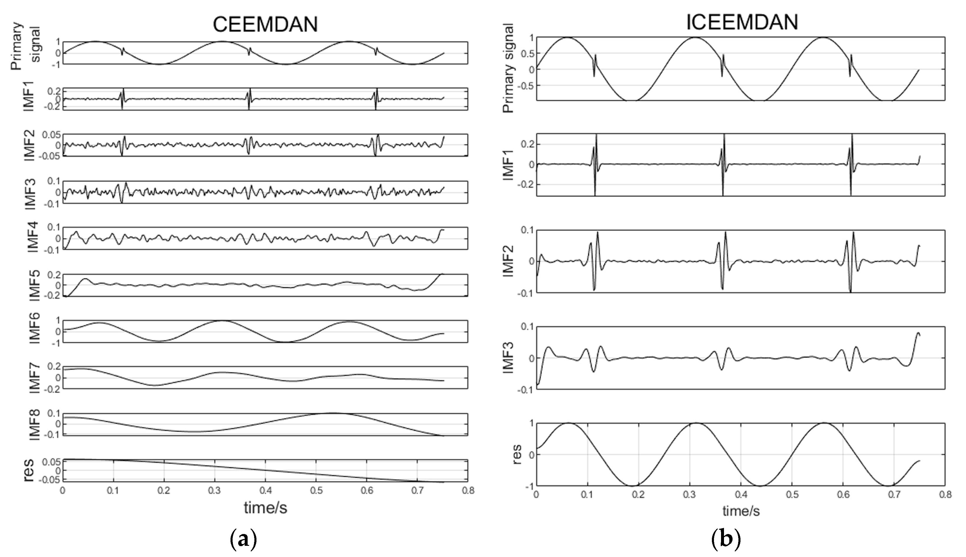
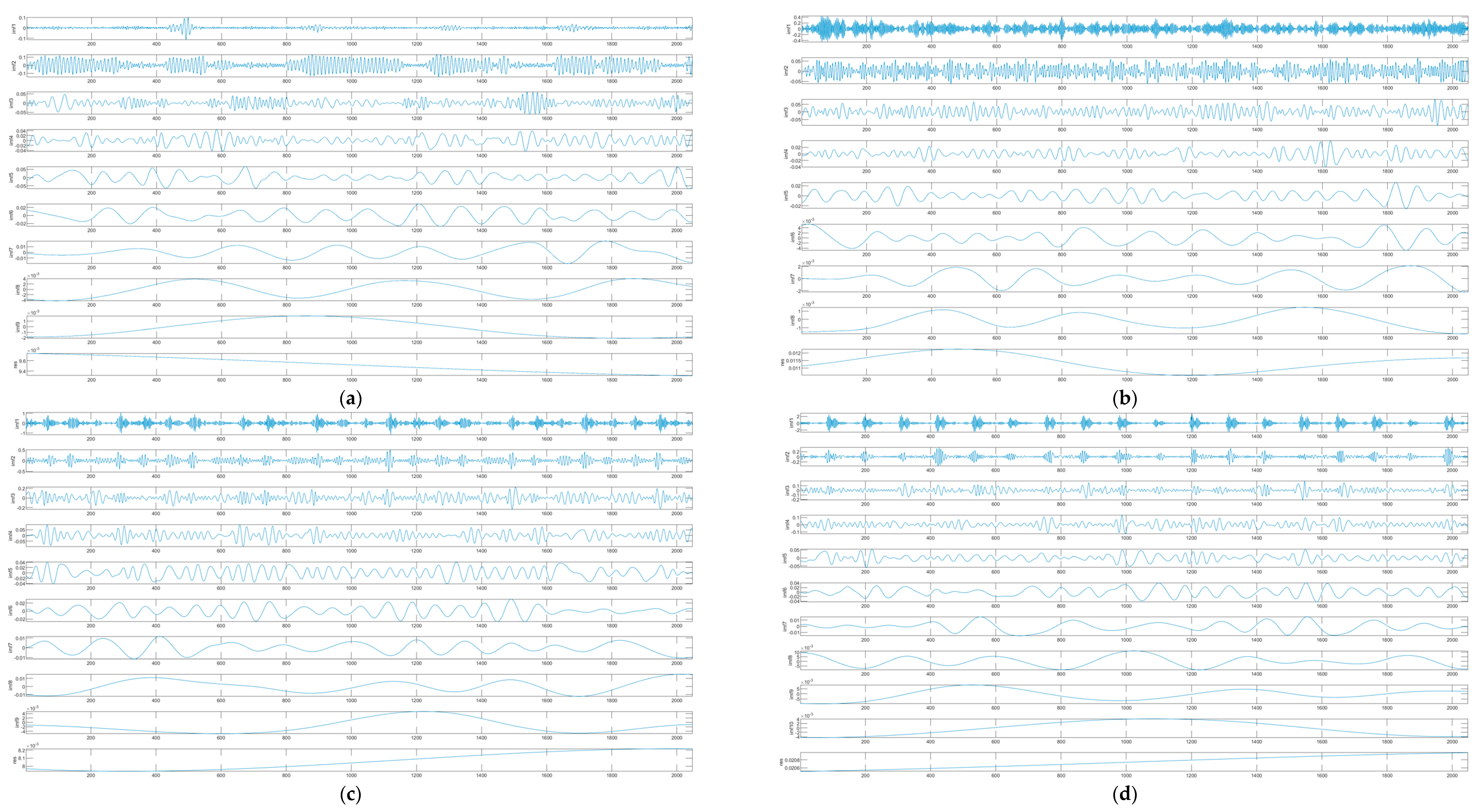
By simulating a sine signal and converting the high-frequency signal into intermittent form, CEEMDAN and ICEEMDAN decompositions were performed, and the decomposition results were compared. Figure 1 shows the decomposition result using CEEMDAN, where it can be observed that IMF1 completely recovers the component of the specially processed high-frequency signal from the original signal, while IMF2 and IMF3 contain residual noise. In IMF6 to IMF10, spurious modes unrelated to the original signal appear. Figure 1b shows the decomposition result using ICEEMDAN, indicating that it is the result of ICEEMDAN decomposition. It can be seen that in IMF1 of the original signal, the high-frequency signal component of the simulated signal, which underwent special processing, is recovered without the presence of spurious modes [11].

2.2. Hilbert Transform Principle

The Hilbert transform essentially converts a one-dimensional signal into a two-dimensional signal [12], or in other words, restores a signal to its original form. Hilbert transform is applied to the IMF components obtained from CEEMDAN, and the specific algorithm is as follows:

For any real-valued function x(t), the Hilbert transform is defined as $\widehat{x}\left(t\right)$, which can be expressed as follows:

$$\widehat{x}\left(t\right)=H\left[x\left(t\right)\right]=\frac{1}{\pi }{\displaystyle {\int }_{-\infty }^{+\infty }\frac{x\left(\tau \right)}{t-\tau }}d\tau$$

(8)

Performing the Fourier transform on the complex frequency domain signal $Z\left(t\right)$,

$$Z\left(t\right)=x\left(t\right)+jH\left[x\left(t\right)\right]$$

(9)

The instantaneous frequency of a signal is defined as the inverse of the time derivative of the phase angle, which corresponds to the concept of frequency in a crucial sense.

$$f=\frac{1}{2\pi }\frac{d\theta \left(t\right)}{dt}$$

(10)

After the decomposition, the IMF components are subjected to Hilbert transform to obtain the Hilbert spectrum. The Hilbert transform allows us to obtain the time-frequency representation and the amplitude-frequency curve of the vibration signal.

2.3. Convolutional Block Attention Module

CBAM is a simple yet effective attention module for feed-forward convolutional neural networks [13]. It is a lightweight and memory-efficient module that can be seamlessly integrated into end-to-end training. As shown in Figure 2, CBAM is a combination of channel and spatial attention mechanisms. Compared to SE-Net, which focuses solely on channel attention, CBAM achieves better results.

By utilizing different neural networks to autonomously learn the importance weights for each channel in the input feature map, the importance levels are assigned different grades. Subsequently, each feature is assigned a weight value based on its importance level, allowing the neural network to focus more on certain feature channels. This improves the emphasis on feature maps that are crucial for the current recognition process while disregarding feature channels of lesser importance.

A spatial attention module [14] is a compression of channels that involves separate average pooling and max pooling operations along the channel dimension. The MaxPool operation extracts the maximum value in each channel, and this extraction is performed for each spatial location (height multiplied by width). Similarly, the AvgPool operation calculates the average value in each channel, and this extraction is also performed for each spatial location (height multiplied by width). Subsequently, the feature maps obtained from the previous operations, each with a single channel, are merged to generate a 2-channel feature map.

2.4. Deep Residual Network

In traditional deep learning models such as VGG and LeNet, as the network depth increases, the nonlinear computational capacity increases, resulting in more features. However, with the increase in network depth, the nonlinear expressions become difficult to be represented by deep network structures as identity mappings. Consequently, traditional network models may suffer from decreased recognition accuracy, gradient vanishing, or gradient explosion issues. In vibration signal data, noise interference and other problems exist, which can affect the accuracy of fault diagnosis in practical applications. This paper proposes the application of deep residual networks for feature extraction and diagnosis of vibration signal spectrograms to address these issues.

Deep residual networks are a type of deep learning method designed for high-noise data [15]. Based on backpropagation training, deep residual networks can propagate gradients layer by layer through convolutional layers and propagate losses through the same mappings as the residual terms. By using soft thresholding to eliminate noise in vibration signals, better models can be obtained.

To address the issues of gradient vanishing or gradient explosion, the ResNet paper suggests using batch normalization [16] (BN) layers in the network and preprocessing the raw data to mitigate these problems.

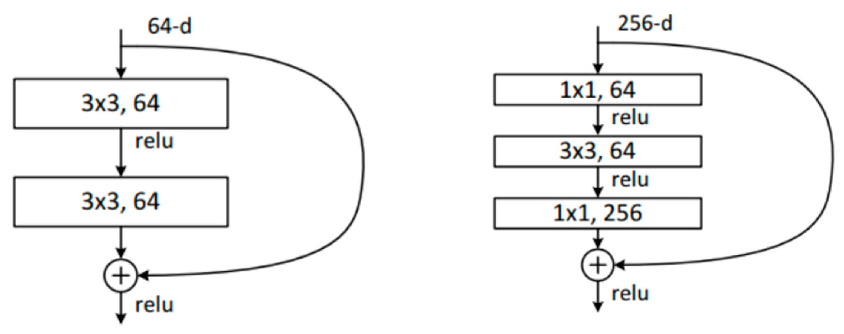
To tackle the degradation problem in deep networks, it is possible to artificially allow certain layers of the neural network to skip the connection to the next layer of neurons, creating skip connections that weaken the strong connections between each layer [17]. The ResNet paper proposed the residual structure to address issues such as gradient degradation. Figure 3 illustrates a convolutional network using the residual structure. As the network depth increases, the recognition results remain good, indicating that the residual network resolves the problem of degraded training performance with increasing depth.

2.5. Transfer Learning

Transfer learning [18] is a term in machine learning that refers to the influence of learning from one task on the performance of another task or the impact of acquired experience on the completion of other activities. Transfer learning is widely present in various forms of knowledge, skills, and social norms learning. It reduces the amount of training data and computational power required to create deep learning models, effectively addressing the problem of overfitting in small datasets in complex networks. Low-level features have strong migration ability, while the features of a high-level convolutional layer are abstract features related to specific tasks, which are not suitable for migration and need to be retrained on new data sets. The implementation of transfer learning can improve the initial performance of the model. The rate of model improvement is faster; in addition, the resulting model converges better.

The key to the success of transfer learning is the similarity between the source domain and the target domain. For similar data sets, training the last fully connected layer will obtain sufficient performance, but the data sets with relatively large differences should be trained to update the parameters of the higher convolution layer.

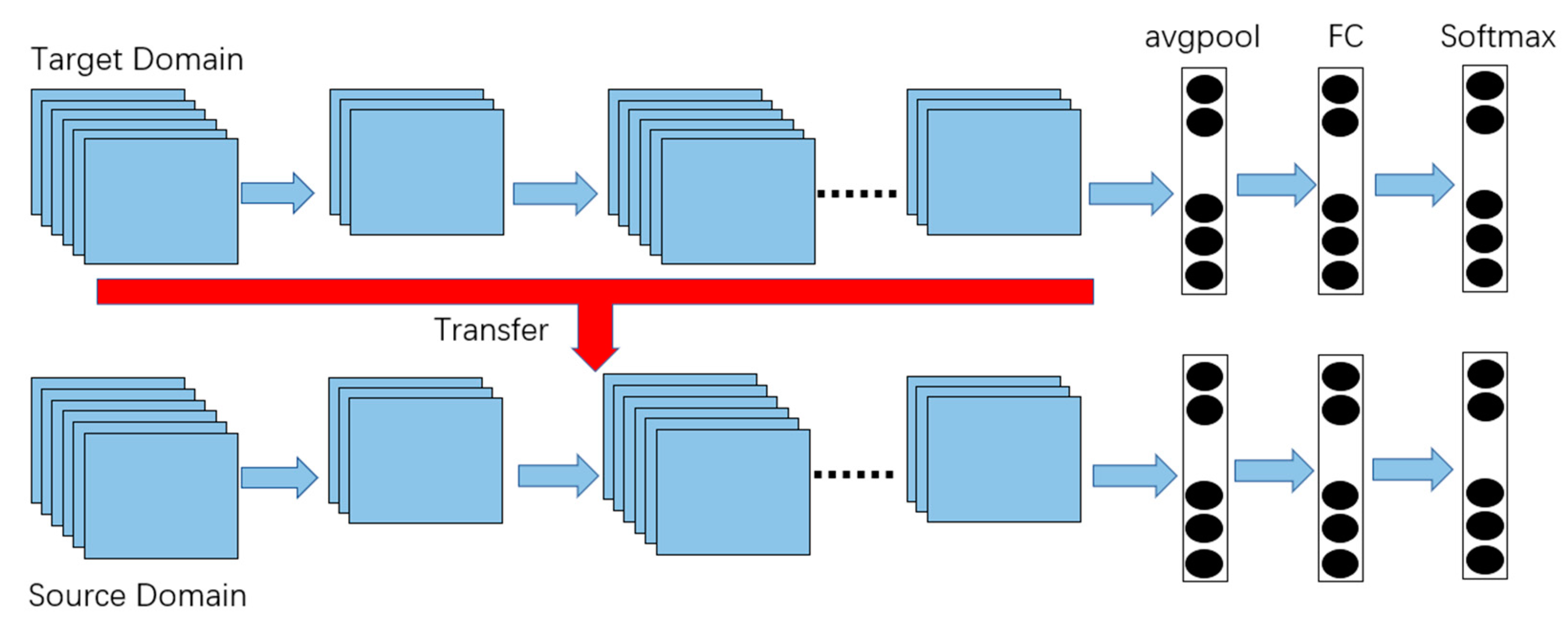
Based on parameter/model transfer learning [19], The source domain is the domain in which data features and feature distribution are known, and the target domain is the domain in which data features and feature distribution are to be learned. The ResNet model belonging to the source domain has been trained on the large-scale image data set ImageNet to obtain the model weights and has achieved good classification results. The trained weight parameters have been transferred to the ResNet-CBAM model of the target domain. Therefore, when the size of the obtained bearing data sample is small, and it is difficult to evaluate the feature extraction using the normal network, the initial weight of the pre-trained model can be used to transfer the experience or knowledge learned by the model in other tasks to the current task. Even if the data set features are different, the features extracted in the training ImageNet, such as edges, textures, shapes, etc., have the same effect on the recognition of images. The parameter weights of some network layers are fine-tuned, including learning rate, loss function, optimizer setting, etc. The modified model weight parameters are suitable for the experimental research in this paper. Using the network weights trained on very large data sets, migrating to your own data for training can save a lot of training time and reduce the risk of underfitting/overfitting. It is assumed that the related models in the source domain and target domain will share some common parameters or prior distributions. This type of transfer learning enables the sharing of part of the model structure between the tasks in the source and target domains, along with their corresponding model structures, as shown in Figure 4.

In this study, the method of transfer learning was employed by freezing certain network layers and fine-tuning some of the layer parameters to pre-train the model.

3. Proposed Method

To investigate the computational performance and accuracy of the proposed fault diagnosis model, the experiments were conducted on a computer server with the following specifications: CPU, Xeon(R) Platinum 8255C (2.5 GHz); memory, 43 GB; GPU, RTX2080Ti 11 GB. The code for ICEEMDAN decomposition and Hilbert transformation was executed in MATLAB 2022a environment. The code for the deep learning network was written and executed in the PyTorch environment.

3.1. Method and Workflow

The proposed ICEEMDAN-Hilbert attention mechanism for bearing diagnosis in the residual network is illustrated in Figure 5. After decomposing the IMF components through ICEEMDAN, the Hilbert transformation converts the one-dimensional time-domain signal into a two-dimensional time-frequency representation. By inputting the network, the fault features of the bearing can be automatically extracted in the time-frequency domain. Transfer learning is employed to transfer parameter weights, where the lower-level convolution layers of the network are frozen, and only the last fully connected layer is trained. This approach improves accuracy and significantly reduces training time. An attention mechanism is introduced before the fully connected layer to explore the channel features, enhance the weights of important information, and ignore less important information channels. This enhances the accuracy of the detection results and achieves the classification of bearing faults.

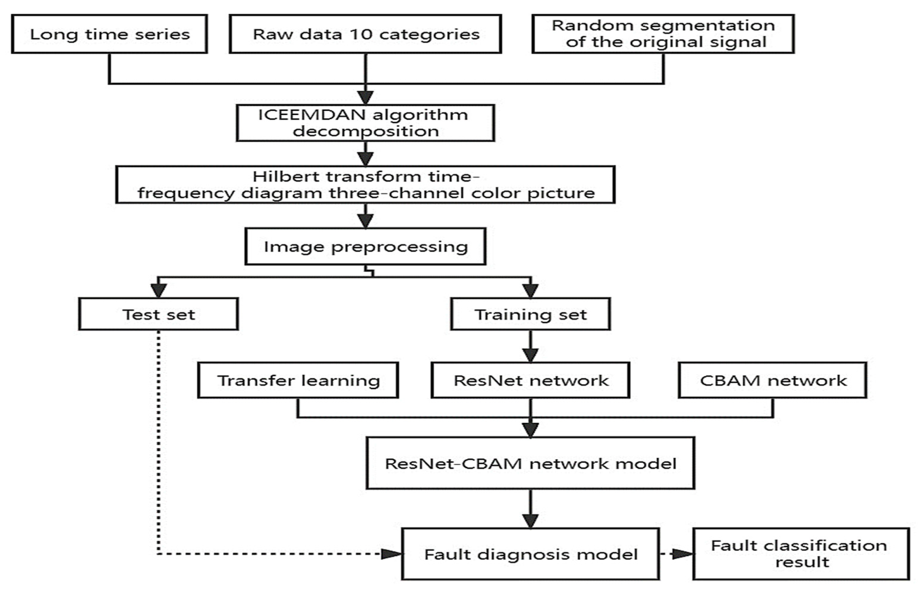
The workflow of the bearing fault diagnosis model based on ICEEMDAN-Hilbert with ResNet-CBAM network is shown in Figure 6. Firstly, the long-time series of composite fault data is collected from a rolling bearing. The raw signal is then randomly divided into non-repetitive segments of fixed length to form fault samples. The samples are further subjected to ICEEMDAN decomposition for denoising, resulting in the IMF components of the original fault vibration signal. The IMF components obtained from the decomposition are then transformed using Hilbert transform, converting the time-domain images into time-frequency images. Preprocessing techniques such as image flipping and cropping are applied. The processed time-frequency images are divided into training and testing sets. The training set is used to train the attention mechanism deep residual network composed of transfer learning, ResNet network, and CBAM network. The fault diagnosis model is optimized through training, resulting in a complete fault model. The constructed fault diagnosis model is then used for recognition, obtaining the recognition results. The effectiveness of the model is evaluated based on the accuracy of fault classification predictions.

3.2. Data Preprocessing of Rolling Bearing

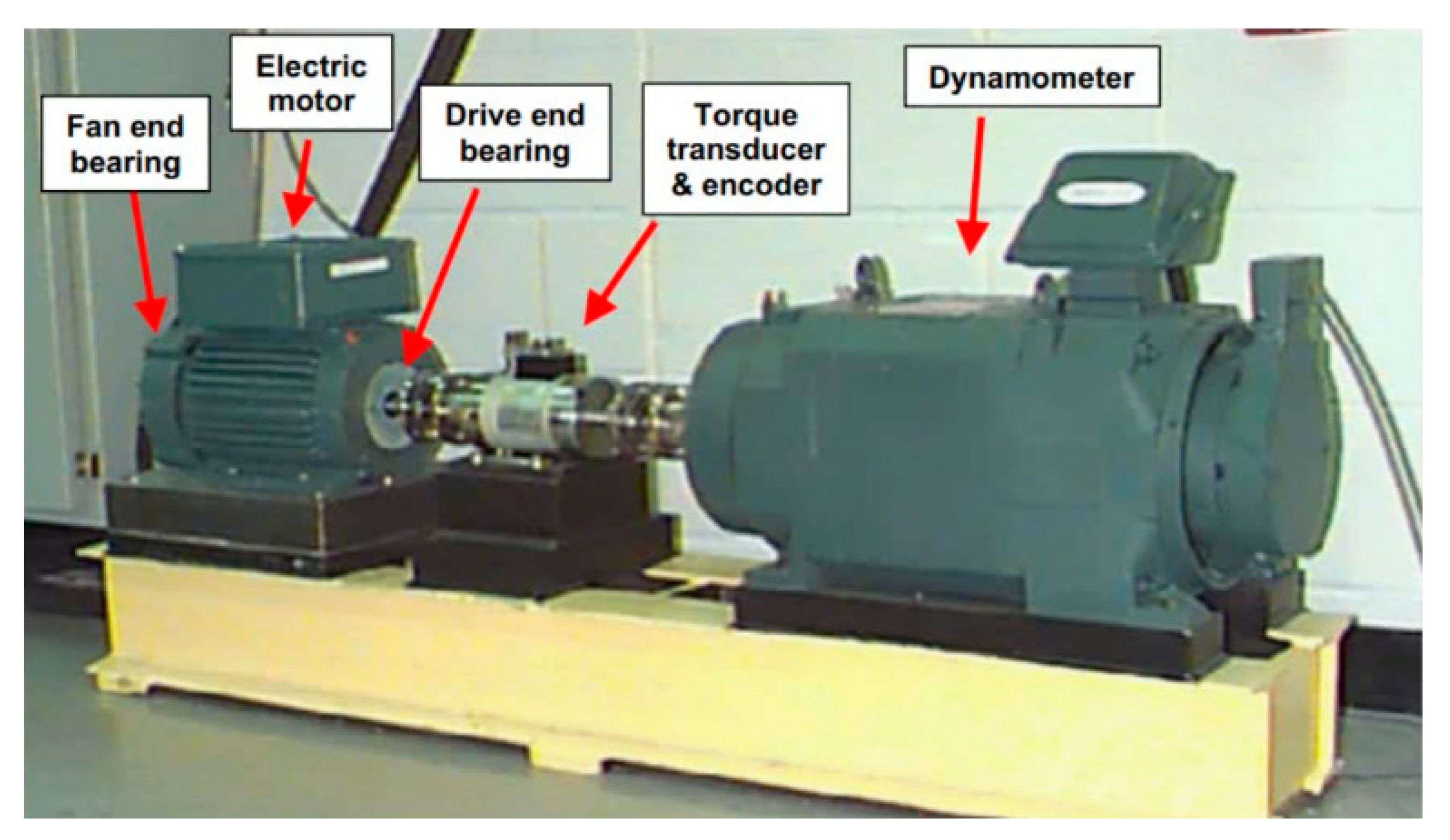
In this study, the rolling bearing dataset from Case Western Reserve University (CWRU) [20] was used for validation, as shown in Figure 7. The experimental platform includes a motor, a torque encoder, a dynamometer, an accelerometer, and other main components. The test bearings support the motor shaft and introduce different types of single-point faults at the drive end (DE) and fan end (FE) with varying fault diameters [21], including 7, 14, 21, and 28 mils. These faults result in single-point faults in the ball, inner race, and outer race. The rolling bearings used in the experiment are produced by SKF, with the specific model being 6205-2RS. The vibration signals from the rolling bearings were collected to acquire fault diagnosis experimental data. A total of three different single-point faults and one set of normal rolling bearing vibration signals were collected at sampling frequencies of 12 kHz and 48 kHz.

The data used in this study was collected on the experimental platform shown in Figure 7. The bearing data was collected at the drive end (DE) under three different load conditions: 0, 1, and 2 (1797 r/min, 1772 r/min, and 1747 r/min, respectively). The collected data was used to construct the dataset, as shown in

Table 1. Classification information of rolling bearings.

Fault Name	Label	Fault Location	Bearing Damage Level/mm	Sample Collection
Normal	0	Normal Bearing	0	3000
007-BALL	1	Ball Fault	0.18	3000
007-IR	2	Inner Race Fault	0.18	3000
007-OUT	3	Outer Race Fault	0.18	3000
014-BALL	4	Ball Fault	0.36	3000
014-IR	5	Inner Race Fault	0.36	3000
014-OUT	6	Outer Race Fault	0.36	3000
021-BALL	7	Ball Fault	0.54	3000
021-IR	8	Inner Race Fault	0.54	3000
021-OUT	9	Outer Race Fault	0.54	3000

. The dataset consists of 30,000 samples, with a split of 80% for the training set (24,000 samples) and 20% for the test set (6000 samples).

For each load condition, tests were conducted on rolling bearings with diameters of 0.18 mm, 0.36 mm, and 0.54 mm, focusing on the ball, inner race, and outer race of the bearings. In addition to the test data for normal rolling bearings, each type of bearing fault was labeled from 0 to 9, resulting in a total of 10 different fault types, including one set of normal bearing data.

In the CWRU dataset, the original vibration signals are segmented into equal-length segments. This allows for the extraction of fault feature information under the same rotating cycle. In this study, each segment consists of 2048 data points, and the starting points of each segment are separated by no less than K data points. In this study, K is set to 100, as shown in Figure 8.

ICEEMDAN is used to decompose the original vibration signals of the bearing into eight IMF components. It can be observed that the first three IMFs obtained from the decomposition by the ICEEMDAN algorithm have relatively high oscillation frequencies. The following five IMFs also have relatively high oscillation frequencies, but compared to the first three IMFs, their oscillation frequencies are lower. Additionally, it can be seen that as the decomposition by the ICEEMDAN algorithm progresses, the oscillation frequencies of the decomposed IMFs become lower. The last IMF and the residual component have very low oscillation frequencies, and the oscillations in the residual component can be neglected. Figure 9 shows the decomposition results of four different conditions (007 mils) using ICEEMDAN, demonstrating that the oscillation frequencies of the obtained IMF components vary with different input signals under different fault conditions. In this experiment, the signal-to-noise ratio (Nstd) is set to 0.2 to ensure continuous mode mixing; the number of noise additions (NR) is set to 100; the maximum number of envelopes inside the EMD process (MaxIter) is set to the default value, resulting in the decomposition of nine IMF components; and SNRFlag is set to 1, indicating ICEEMDAN decomposition when the value is 1 and CEEMDAN decomposition when the value is 2.

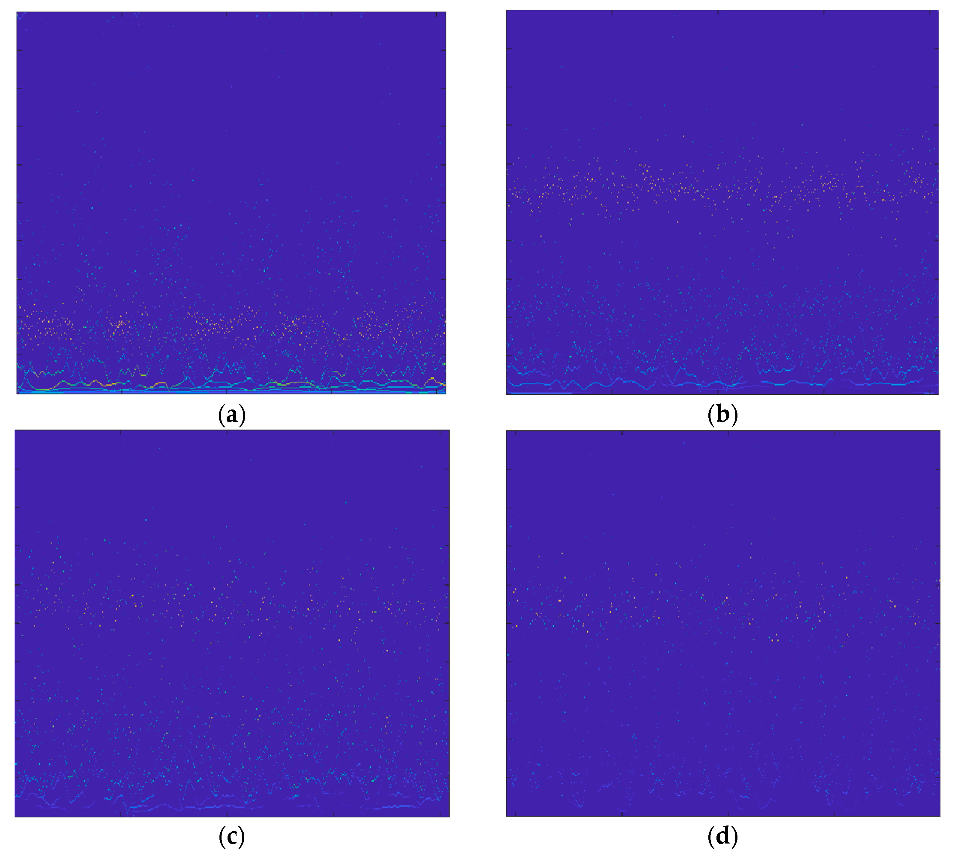
For the Hilbert transform on the basis of ICEEMDAN, each IFM component value is calculated by Hilbert transforming to its Hilbert spectrum; based on each IMF component value and its corresponding Fourier spectrum, the instantaneous frequency fault characteristics of the rolling bearing are mapped on the map, and finally, the Hilbert spectrum is obtained. It can be seen that the feature distribution in the time-frequency diagram is not the same; the distribution of noise points is denser in the ball fault, the distribution under normal conditions is relatively uniform, and the fault ripple and noise points of each kind are obviously different. This is shown in Figure 10. After the Hilbert transform of the vibration signal, the amplitude and frequency of the vibration signal are time functions, and the amplitude is reflected in the time-frequency diagram, and the Hilbert spectrum of the amplitude is represented by contours. A complex exponential signal can be represented as the sum of a real signal and an imaginary signal, and the result of converting a real signal into an analytical signal is that a one-dimensional signal is converted into a signal on a two-dimensional complex plane, and the amplitude and phase of the signal are represented by the modulus and amplitude angles of the complex number. Compared with other signal processing methods, this method has the advantages of being able to decompose unstable signals and being adaptive.

3.3. Diagnostic Results of the ResNet-CBAM Network Model

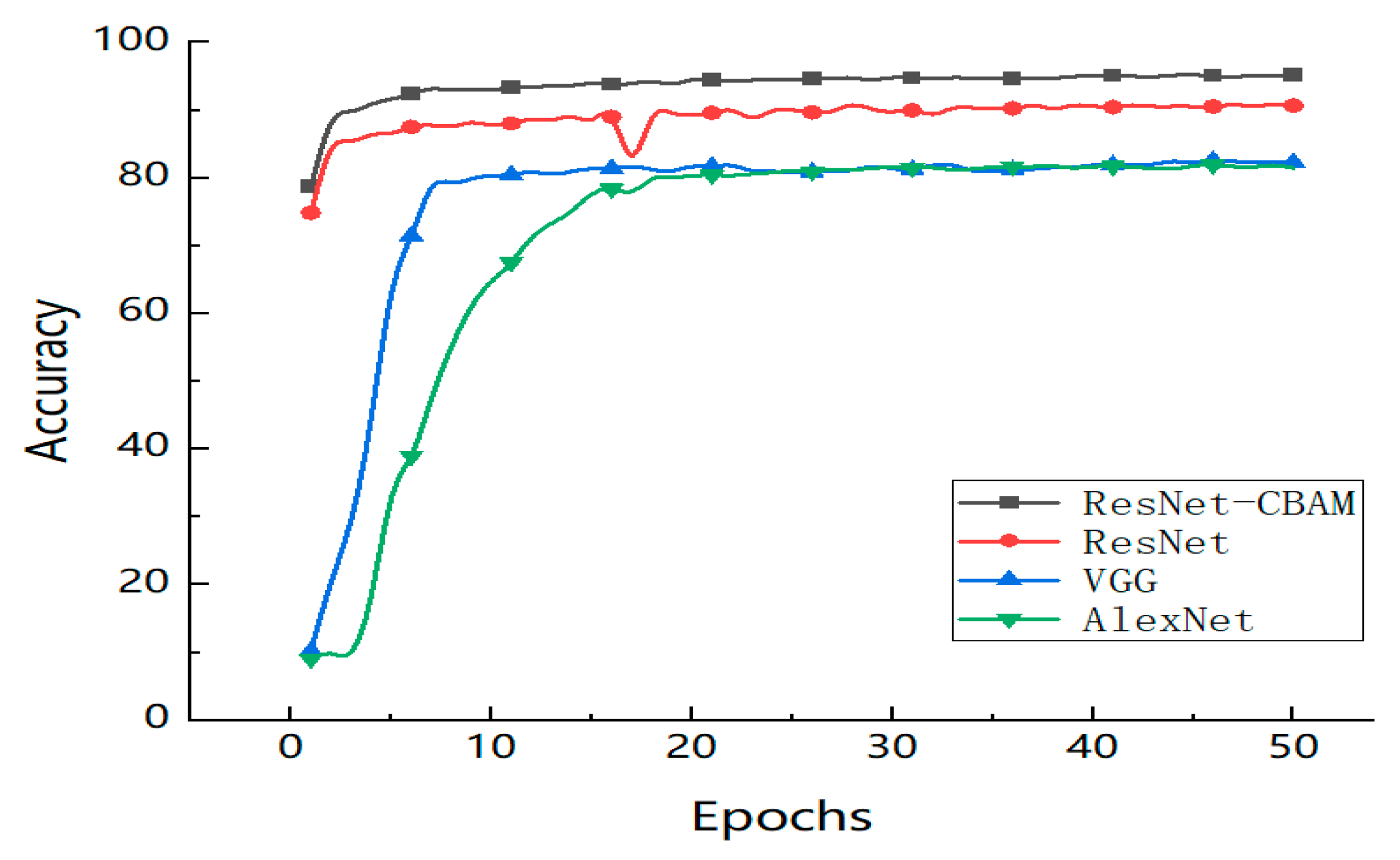
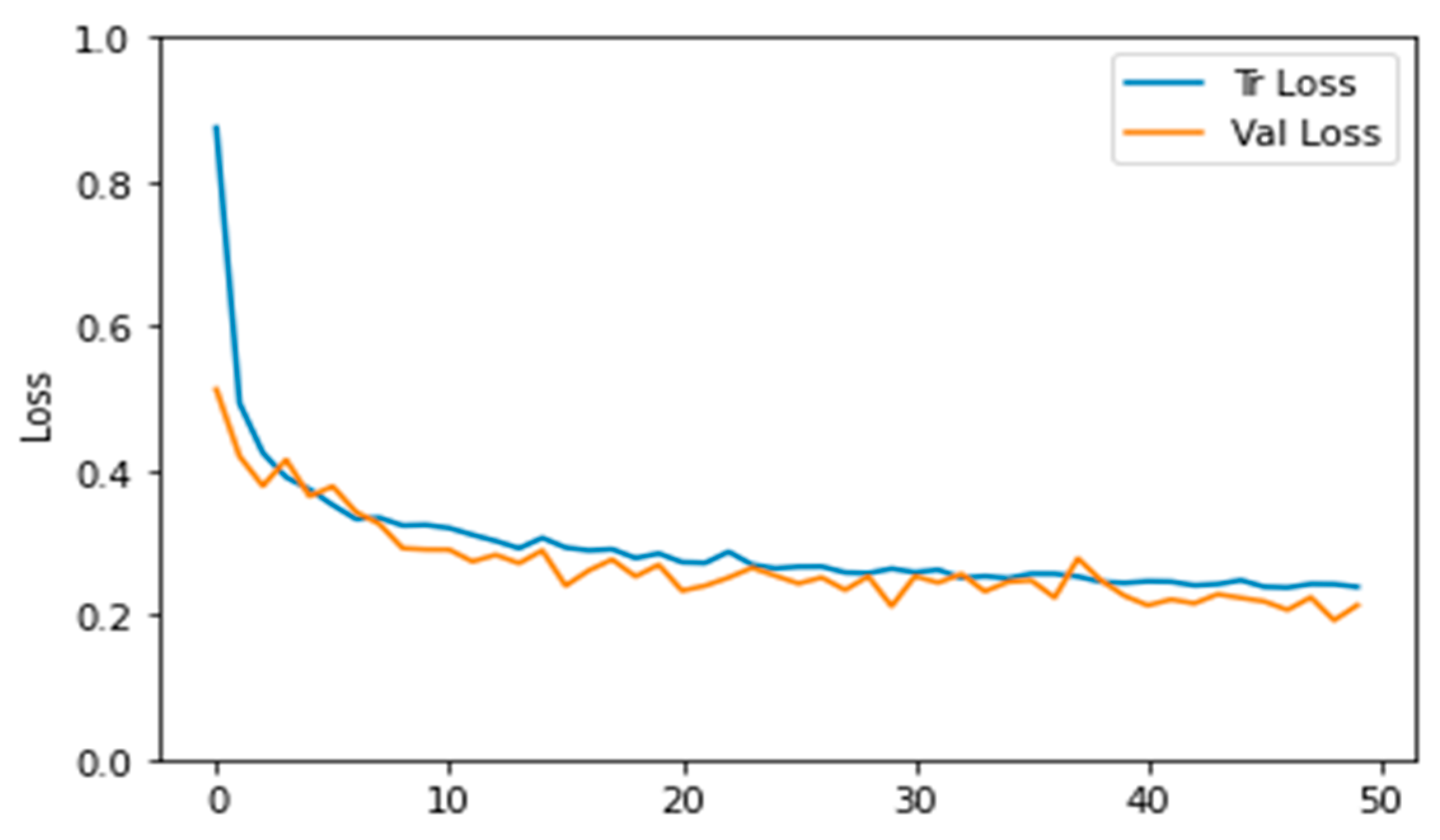
In the experiment, a network model was constructed using PyTorch. Ten sets of data were randomly sampled, and each set consisted of 128 randomly selected images. These images were then randomly cropped to a size of 256 × 256 and input into the model for training. The model was trained on a GPU for 50 epochs to validate its reliability. The accuracy of the final model training output was 95.2%, as shown in Figure 11. This accuracy surpasses not only the regular ResNet network but also the accuracy of VGG and AlexNet by more than 12%, demonstrating that the accuracy of this model has reached the expected level. The loss rate of ResNet-CBAM is around 0.2, as shown in Figure 12.

Table 2. The comparative experimental results of the four models after 50 epochs of training.

Model Name	Model Accuracy/%	Loss Rate
VGG	0.823	1.2
ResNet	0.907	0.36
AlexNet	0.814	0.83
ResNet-CBAM	0.952	0.19

compares the classification prediction accuracy of the four models and provides the corresponding loss rates for each condition in the respective methods. From Table 2, it can be concluded that the combination of ICEEMDAN-Hilbert and ResNet-CBAM models achieves good classification accuracy and reduces computational loss rates. It can accurately address the complex fault classification problem of bearings, proving the feasibility and applicability of this method in practical applications.

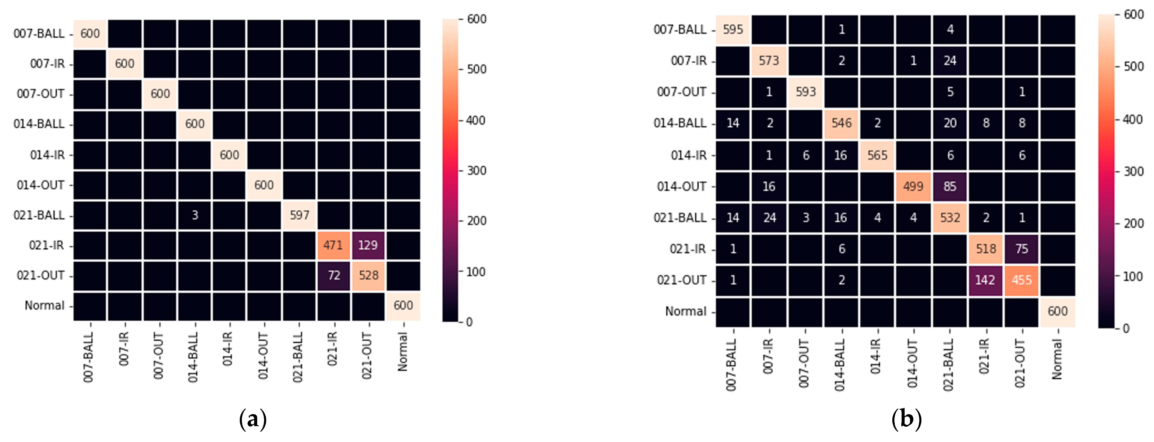
Furthermore, the distribution of fault misjudgment information in this model is further demonstrated. In this study, a multi-class confusion matrix was introduced to analyze the effect of fault diagnosis. The confusion matrix effectively reflects the diagnostic accuracy and the specific number of misjudgments in various types of rolling bearings, such as the misjudgment of actual fault types into specific types. The confusion matrix is shown in Figure 13.

In Figure 13a, the predicted fault categories are represented by the x-axis, while the true fault labels are represented by the y-axis. Each category consists of 600 test samples, totaling 10 fault types. The numbers on the main diagonal represent the number of samples correctly diagnosed by the ResNet-CBAM network model algorithm for each fault type. In Figure 13a, among the 6000 samples in the test set, samples from 021-OUT, 021-IR, and 021-BALL were predicted incorrectly. The misclassified samples had the true label of 021-BALL (21 mils ball fault) but were predicted as fault category 014-BALL (14 mils ball fault). Similarly, misclassified samples with the true label of 021-IR (21 mils inner ring fault) were predicted as fault category 021-OUT (21 mils outer ring fault), and misclassified samples with the true label of 021-OUT were predicted as fault category 021-IR. Additionally, the diagnostic accuracy for other fault types was 100%.

The confusion matrix for the normal ResNet network is shown in Figure 13b, which is noticeably different from Figure 13a. Only the normal samples were predicted correctly, while each class of fault samples had varying degrees of diagnostic errors. For the 021-BALL (21 mils ball fault), each fault category exhibited different levels of recognition errors. However, in the ResNet-CBAM network algorithm, there were no such diagnostic errors for the 021-BALL (21 mils ball fault) class. The recognition was correct without any errors.

The experimental data above demonstrate that the proposed ResNet-CBAM network algorithm, with the support of transfer learning, possesses high computational capability. It achieves a higher fault recognition rate than ordinary deep learning networks under different load conditions and accurately identifies the location of faults. This is of significant importance for the fast localization and diagnosis of faults in rolling bearings, targeted maintenance, and optimization improvement for multi-fault components.

4. Conclusions

In this paper, an algorithm for fault diagnosis of rolling bearings combining ICEEMDAN decomposition of vibration signals, transformation of decomposed IFM components into RGB images using the Hilbert transform, and the integration of attention mechanism with deep residual networks (ResNet-CBAM) is proposed. It can be applied to the fault diagnosis of rolling bearings under different environmental conditions through transfer learning:

(1) When facing long time series vibration data of rolling bearings and complex fault situations composed of multiple mixed signals, transforming the one-dimensional vibration signal data matrix collected from rolling bearings into two-dimensional Hilbert time-frequency map fault samples facilitates deep learning training of this model.

(2) For the entire process from normal state to failure of rolling bearings, a method of random sampling with multiple sampling points is adopted to construct life-cycle fault samples for fault diagnosis.

(3) A multi-layer convolutional network framework model combined with the attention mechanism (CBAM) is used to diagnose rolling bearing faults and extract deep features from various types of vibration signal data for different fault types.

(4) The fault data of rolling bearings from different categories are reflected in the CWRU dataset, and ResNet-CBAM achieves high fault diagnosis accuracy in the experiments. Based on the results of this model, it can be applied to fault diagnosis of rolling bearings under various operating conditions. To obtain more accurate fault diagnosis results and improve the robustness of the model, training with a larger variety of samples will be conducted, and the possibility of incorporating residual modules into various deep learning model frameworks will be explored.