Article

Machine Learning-Based Prediction of Controlled Variables of APC Systems Using Time-Series Data in the Petrochemical Industry

1
Department of Smart Factory Convergence, Sungkyunkwan University, 2066, Seobu-ro, Jangan-gu, Suwon 16419, Republic of Korea
2
Infotrol Technology, 159-1, Mokdongseo-ro, Yangcheon-gu, Seoul 07997, Republic of Korea
3
Department of Statistics, Sungkyunkwan University, 25-2, Sungkyunkwan-ro, Jongno-gu, Seoul 03063, Republic of Korea
4
Department of Chemical Engineering, Sungkyunkwan University, 2066, Seobu-ro, Jangan-gu, Suwon 16419, Republic of Korea
5
Department of Mechanical Engineering, Sungkyunkwan University, 2066, Seobu-ro, Jangan-gu, Suwon 16419, Republic of Korea
6
Department of System Management Engineering, Sungkyunkwan University, 2066, Seobu-ro, Jangan-gu, Suwon 16419, Republic of Korea
7
Department of Computer Science and Engineering, Sungkyunkwan University, 2066, Seobu-ro, Jangan-gu, Suwon 16419, Republic of Korea
*
Author to whom correspondence should be addressed.
Processes 2023, 11(7), 2091; https://doi.org/10.3390/pr11072091
Submission received: 13 June 2023 / Revised: 4 July 2023 / Accepted: 10 July 2023 / Published: 13 July 2023

Abstract

:
For decades, the chemical industry has been facing challenges including energy conservation, environmental protection, quality improvement, and increasing production efficiency. To address these problems, various methods are being studied, such as research on fault diagnosis for the efficient use of facilities and medium-term forecasting with small data, where many systems are being applied to improve production efficiency. The problem considered in this study is the problem of predicting time-series Controlled Variables (CV) with machine learning, which is necessary to utilize an Advanced Process Control (APC) system in a petrochemical plant. In an APC system, the most important aspect is the prediction of the controlled variables and how the predicted values of the controlled variables should be modified to be in the user’s desired range. In this study, we focused on predicting the controlled variables. Specifically, we utilized various machine learning techniques to predict future controlled variables based on past controlled variables, Manipulated Variables (MV), and Disturbance Variables (DV). By using a time delay as a parameter and adjusting its value, you can analyze the relationship between past and future data and improve forecasting performance. Currently, the APC system is controlled through mathematical modeling and research, The time-series data of controlled variables, manipulated variables, and disturbance variables are predicted through machine learning models to compare performance and measure accuracy. It is becoming important to change from mathematical prediction models to data-based machine learning predictions. The R-Squared (R2) and Mean Absolute Percentage Error (MAPE) metric results of this study demonstrate the feasibility of introducing an APC system using machine learning models in petrochemical plants.

1. Introduction

Petrochemical plants process raw materials related to petroleum to produce various chemicals. These plants utilize a variety of processes—including petroleum refining, chemical reactions, separation, and purification—to produce a variety of consumer products, including plastics, fibers, polymers, artificial rubber, and lubricants. Petrochemical plants are recognized as a globally important industry, contributing to energy, economies, and industrial development.
In general, the types of plants can be divided into intermittent and continuous processes. Among them, most petrochemical plants utilize continuous processes, where many substances are introduced continuously at the same time, and the quality of the product varies depending on the influence of each substance [1,2]. Many continuous process petrochemicals are controlled using Proportional Integral Differential (PID) control, which is a feedback control technique that does not consider multiple variables [3]. Since this approach does not consider multiple variables, there has been a trend of switching to Advanced Process Control (APC), which is a feedforward control with excellent performance [4]. APC systems are advanced control technologies used in process and manufacturing systems to control the complex behavior of processes by utilizing advanced mathematical modeling and optimization algorithms. This is due to the inclusion of Model Predictive Control (MPC), which is a technology that optimizes control behavior by considering various constraints based on future prediction models. APC, including MPC technology, enables more accurate control by controlling the relationship between the Controlled Variables (CV) to be controlled and the Disturbance Variables (DV) that cannot be controlled as well as the Manipulated Variables (MV) that can be controlled with a model [5]. In addition, real-time monitoring, feedback control, and limit condition management control functions are used to improve accuracy. The application of such systems and control methods aims to address the issues faced by not only the petrochemical industry but also the overall chemical industry, including energy conservation, environmental protection, quality improvement, and increasing production efficiency [6,7].
The benefits of switching to an APC system, such as increased production and reduced costs, have been documented in several papers. In the oil industry, APC systems have been utilized to increase crude oil production by 10% [8], and in the petroleum refining industry, APC systems have been applied to improve planning system performance [9,10]. In the petrochemical industry, where the data for this paper was obtained, APC systems have also been applied to minimize cost-effective glycol losses in natural gas dehydration plants [11]. APC systems are also being used in technologies that control the indoor environment in buildings. We quantified the number of papers involving efficiency improvements by applying APC systems for heating, ventilation, and air conditioning (HVAC), and found that the number of papers reporting energy savings of 10.1–15% by applying APC and MPC compared to conventional control systems was the highest with 17, followed by 20.1–25.0% with 13. A total of 80 cases were investigated [12,13,14].
The APC system introduced earlier has the disadvantage of not being able to respond to changes in factory equipment or conditions because the data is created with only the factory conditions at the time the model was created. Moreover, it does not respond to the decline in performance due to aging facilities and does not consider the temperature difference between summer and winter. Therefore, it is necessary to study the data of the current factory conditions to predict the controlled variables of the APC and manipulate them by entering the optimal values of the controlled variables. In this study, we investigated the controllability by learning the time-series data with machine learning and improving the control accuracy.
Prediction of time-series data through machine learning is already being actively studied in various fields. For example, time-series data prediction is used to predict climate variables such as rainfall [15], wind speed [16], and other phenomena [17]. In the financial field, stock price prediction is also being actively studied [18,19]. The petrochemical industry is also active in this area, with researchers using artificial neural networks to predict the production of petrochemical products [20] and to predict the temperature of distillation columns [21,22,23,24].
The major contributions of this paper can be summarized as follows: First, we solved the problem of predicting controlled variables in APC systems with machine learning and confirmed its feasibility. Second, the performance of feature engineering for predicting controlled variables was determined. Feature engineering is the process of extracting new features from existing data that are easier for a prediction model to learn. It is a method utilized to improve prediction performance. Finally, comparison of multiple machine learning models was carried out. A variety of machine learning models were applied, including Random Forest, Neural Network, k-Nearest Neighbor, Support Vector Regression, and XGBoost. The R-Squared and MAPE squared metrics were applied to find the model with the best predictions.
The rest of the paper is organized as follows. Section 2 describes PID and APC systems for process control in more detail and introduces the machine learning algorithms used in this study. Section 3 presents an overview of this study and describes the time-series data from a petrochemical plant and the feature engineering for it. We also present the modeling and hyper-parameter tuning process of the machine learning models used in this study. In Section 4, we present and evaluate the performance of the machine learning models based on the datasets and evaluation metrics used in the experiments. Conclusions are given in Section 5, along with plans for future work.

2. Background

2.1. APC System

2.1.1. PID System

The Classical Controller consists of an On/Off control where the most commonly used control techniques are P, PI, and PID control. PID control, which stands for Proportional–Integral–Derivative control, is a common control algorithm widely used in automatic control systems. PID control measures the current state of the system and calculates control inputs based on that to maintain or regulate the system at a desired target state. P control is proportional control, meaning that it generates control inputs that are proportional to the error between the current state and target state. The error cannot be eliminated, so the exact target state may not be reached. PI control is a control method that adds integral control to P control. The integral control calculates the accumulated error and adjusts the control input. The integral action, which can cause instability in the system, must be controlled. PID control is a control method that adds differential control to the functions of P control and PI control. A block diagram for PID is shown in Figure 1. Differential control tracks the rate of change of the error and adjusts the control input. This allows the system instability to be predicted and the control input to be adjusted appropriately to improve the response time and reduce oscillations [4,6].

2.1.2. APC System

Advanced Process Control (APC) is a type of control algorithm that uses a system behavior model to predict the future sequence of control inputs and selects the optimal control input at the current time based on it. It is a set of control techniques used in the field of process control [25,26]. APC aims to improve the performance and maintain the stability of the process by utilizing various control algorithms, modeling techniques, and optimization techniques. APC includes model predictive control (MPC), which uses mathematical models to predict the dynamic characteristics of a process, optimization techniques [27,28], multivariable control, which manipulates multiple variables simultaneously, real-time monitoring, feedback control, and constraint management control [10,29].
Among the functions of APC, model predictive control (MPC) refers to a class of algorithms that calculate a series of manipulated variable adjustments to optimize the plant’s behavior. A block diagram of APC is shown in Figure 2 below. Industrial MPC controllers typically evaluate the future CV behavior over a finite future time interval called the prediction horizon [7]. APCs are widely used in industry to automate and optimize processes, providing benefits such as energy efficiency, increased productivity, and improved quality.
The procedure for building an APC is as follows: (1) From the stated control objectives, define the size of the problem and determine the relevant CVs, MVs, and DVs. (2) Test the plant systematically by varying the MVs and DVs, and capture and specify real-time data showing how the CVs respond. (3) Derive a dynamic model from the plant test data using an identification package. (4) Configure the MPC controller and enter the initial tuning parameters. (5) Test the controller off-line using a closed-loop simulation to verify the controller performance. (6) Download the configured controller to the destination machine and test the model predictions in the open-loop mode. (7) Commission the controller and refine the tuning as needed [7].

2.2. Machine Learning Algorithm

2.2.1. Random Forest

Random Forest (RF) is a representative supervised learning model that combines multiple decision trees in a bagging fashion to overcome the limitations of individual decision trees [30]. RF is a machine learning algorithm that uses multiple decision trees for training and can be applied to classification and regression problems [31]. For classification problems, it outputs the most predicted value of the decision trees, and for regression problems, it outputs the average of the predicted values of the decision trees [32]. In addition to simple regression problems, RF is used to predict time-series data, with examples in engineering, environmental and geophysical sciences, and finance [33]. RF belongs to the bagging type, which increases the diversity of the tree by growing it from different subsets of training data generated through techniques that train data generation by resampling existing data sets largely at random [29]. Because bagging uses independent random vectors with the same as the input samples to generate the subsets, some data can be used for training only once, while others can be used multiple times. Therefore, greater stability is achieved because it can react more robustly to changes in the data and increase prediction accuracy. RF, on the other hand, uses the best features/bifurcation points within a randomly selected subset of evidence features from the entire set of input evidence features when growing the tree. Thus, this may reduce the strength of any single tree, but it also reduces the correlation between trees, which reduces the generalization error. RF can compute an unbiased estimate of the generalization error without using an external subset of text data. RF also provides an assessment of the relative importance of different evidential features [31]. This aspect is useful for multi-source studies where data dimensionality is very high. It is important to know how each feature affects the predictive model so that the best evidential features can be selected.

2.2.2. Support Vector Regression

SVR solves linear regression problems by mapping data points into a higher dimensional space. SVR works by building a regression model that maximizes the margin between the given data points and a line or curve. SVRs use loss functions that predict continuous values, solve regression problems, and minimize residual errors; SVMs use loss functions that maximize margins to predict discrete class labels, solve classification and regression problems, and build classification models [34,35].

2.2.3. Neural Network

A Neural Network (NN), also known as an Artificial Neural Network (ANN), is an information management model that resembles the functioning of the biological nervous system of the human brain. NNs are structured to operate in the same way that an efficiently functioning human brain performs tasks. They have a structure that mimics the neurons and synaptic relationships between neurons in the human brain. Similar to the process of human learning, NNs require adjustments to the relationships between nodes in the layers that function as neurons in order to learn. NN layers are independent of each other, and any given layer can have an arbitrary number of nodes. An arbitrary number of nodes is called a bias node and a bias node is equivalent to an offset in a linear regression. The main function of a bias node is to provide the nodes with a trainable constant value in addition to the normal input that the network nodes receive [36]. With this mode of operation, NNs have been extensively applied to real-world problems in business, education, economics, and life issue applications. They are effective algorithms for identifying trends in data and patterns, which is what we are trying to identify in this study.

2.2.4. K-Nearest Neighbor

K-Nearest Neighbor (k-NN) is a non-parametric method used for classification and regression and is classified as a lazy learner because it does not store instances during the training phase. Given some features, such as the explanatory variables of a new instance to be classified (regression), k-NN finds the k training instances closest to the new instance based on some distance metric and returns the average explanatory variable, which is the majority class. The basic explanation for using k-NNs for time-series prediction is that since all time-series data contain repetitive patterns, we can find previous patterns that are like the current time-series structure and use subsequent patterns to predict future behavior [37]. Since our goal in this study is to identify patterns in time-series data to predict future patterns, we used k-NN to identify patterns in time-series data.

2.2.5. XGBoost

The XGBoost (XGB) algorithm is based on the Gradient Boosting Framework, which builds tree ensemble models to make predictions. XGB trains each tree sequentially using gradient descent on the training dataset and updates the model in a way that minimizes the residual error. This allows XGB to improve prediction performance and avoid overfitting. It also provides a variety of features to improve the generalization performance of the model and enhance its speed and memory efficiency [38].

2.2.6. Benefits of Machine Learning Algorithms

Machine learning can be used as a powerful tool for continuous quality improvement in large-scale, complex processes such as semiconductor manufacturing. Since manufacturing often involves dealing with high-dimensional data, machine learning algorithms have the advantage of being applicable to such high-dimensional problems. Another advantage of machine learning technology is the ease of use of algorithmic applications due to the variety of programs available. They can be easily applied to many processes, even in petrochemical plants. Furthermore, the classification performance can be increased by adjusting the parameters. The main advantage of machine learning algorithms is that they can uncover new, previously unknown knowledge and identify relationships in a data set. This new information can be used to support engineers’ decisions or improve the system [39].

3. Proposed Idea

3.1. Overall Architecture

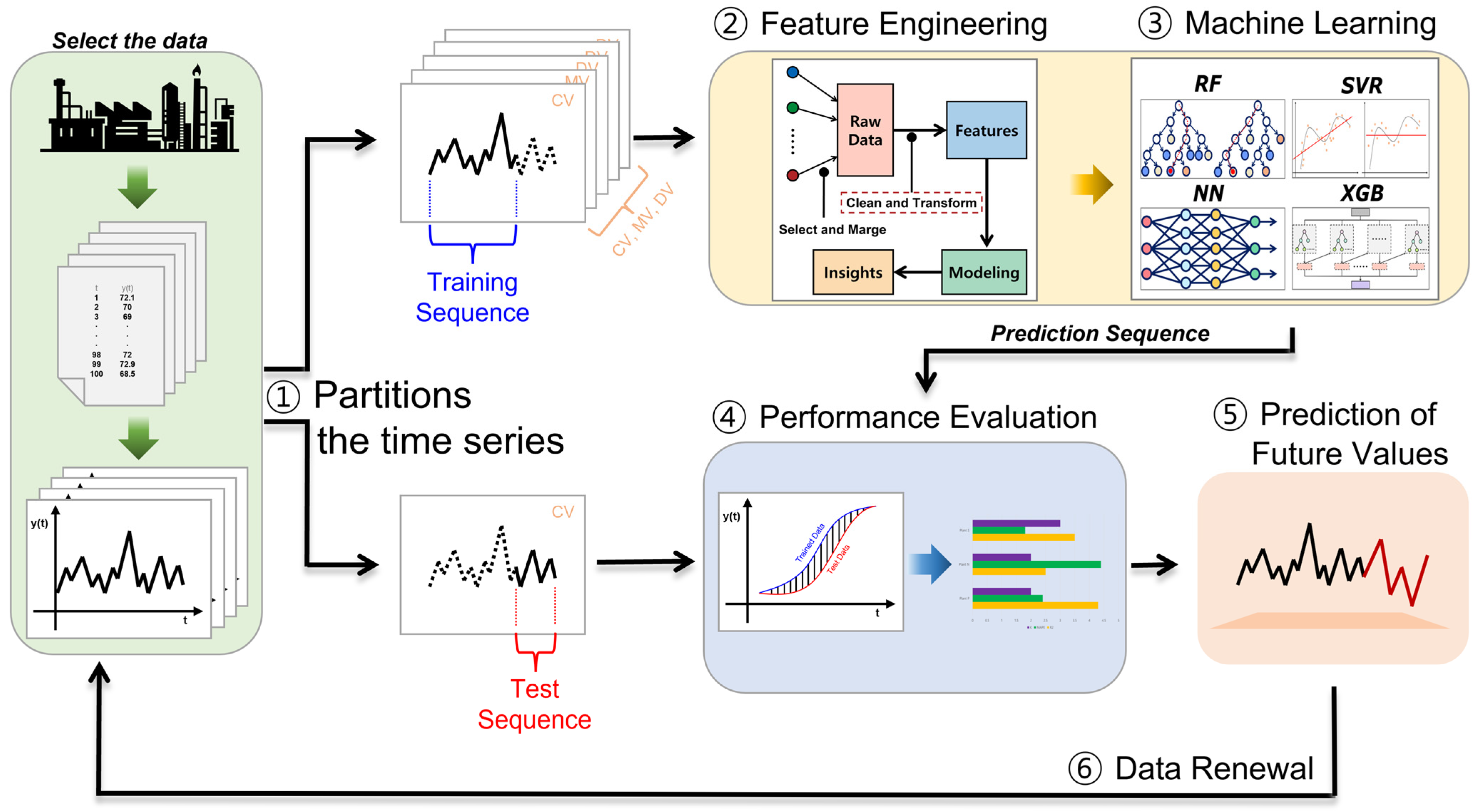
In the petrochemical industry, a machine learning-based controlled variable prediction technique for APC systems using time-series data involves six steps, as shown in Figure 3 [40].
In the first step, we partition the data into two sequences. The data include the controlled variables that the petrochemical plant wants to control with the APC system, the uncontrollable disturbance variables, and the controllable regulated variables. One sequence of data is partitioned before the prediction horizon of the control, regulated, and disturbance variables for machine learning purposes. The other sequence is partitioned after the prediction horizon, which is used to evaluate the quality of the fitted model. The data partitioned for machine learning purposes include controlled variables, moderators, and disturbance variables, while the data partitioned for quality assessment include only the controlled variables to be predicted. In the second step, feature engineering is set up on the time-series data. Feature engineering uses mean, standard deviation, skewness, kurtosis, maximum, minimum, and change in mean to generate useful features or variables from the raw data. The features generated through the feature engineering process provide new information to the model that was not present in the original raw data. This enables the model to make more accurate predictions. Additionally, the selected features are used in the feature selection process to extract the necessary information for model training. In the third step, we define the models, transform the data, and train them with machine learning models. To use different regression models such as RF, NN, k-NN, SVR, and XGB, we define a model grid and set up a hyperparameter grid for each machine learning model. After that, we transform the data according to the given time and prediction time and use the data from the previous time to generate the statistical characteristics of each variable. For each variable, we select the important variables and train the model based on the selected variables. The fourth step measures the accuracy by comparing the predicted values to the evaluation sequence. This step uses the R-Squared (R2) and Mean Absolute Percentage Error (MAPE) metrics to compare the hyperparameter combinations. The fifth step is to predict future periods of the time series. It should be monitored against actual values and aims to indicate when the model needs to be updated with new data or re-parameterized because the distribution of newer data is distinct from older data. The sixth step is to update with new data. In petrochemical plants, the turnaround period is when production is stopped and all facilities in the plant are inspected for maintenance, equipment improvement, noise control, safety checks, and so on. During the turnaround period, the performance of the plant may improve, and the time-series predictions of the APC controlled variables may not be correct. Therefore, it is necessary to retrain with new data and find hyper-parameter combinations.

3.2. Time-Series Data and Feature Engineering Method

Time-series data is sequential data derived from observations of N variables over a period of time. Examples include stock prices, precipitation, and traffic data. Time-series data forecasting predicts the future behavior of an objective variable based on data obtained from past data observations. Time-series data forecasting is used in a variety of fields and has many applications in finance, transportation, engineering, health, and weather, among others [41,42]. Feature engineering is the process of extracting new features from existing data that are easier for a prediction model to learn. It is an important step in machine learning and data analytics in particular, as it is the process of generating useful features or variables from raw data. Feature engineering involves various tasks such as data cleaning, scaling, outlier handling, and transforming and combining different features.
In this paper, feature engineering is very important in time-series modeling, including time-series prediction, to accurately express the meaning of the time series, and it is necessary to analyze the meaning of the prediction on what basis it was made. Therefore, the following features are generated for each variable, and the top k (k = 10, 20, 30, …) features are selected for modeling based on the R2 score of the simple regression model. Table 1 shows the features we considered:
Removing rows with missing values is necessary to ensure the validity of the data. Rows with missing values cannot be used for training, so removing them refines the data. Additionally, by calculating the moving average and standard deviation, trends and volatility in the data can be incorporated into the model. Skewness and kurtosis can also be calculated to reflect the characteristics of the distribution in the model. By calculating the minimum and maximum values, the range of the data can be incorporated into the model to improve the scaling or normalization efforts. Finally, by calculating the mean difference, time-series characteristics can be incorporated into the model. These feature engineering tasks can improve forecasting performance.

3.3. Hyper-Parameter Grid

In this study, we address the problem of predicting the desired controlled variable based on one or more uncontrollable disturbance variables and controllable regulatory variables using various machine learning models, as shown in Equation (1):
y ^ t + τ 2 = f ( x t τ 1 , , x t , z t τ 1 , , z t , y t τ 1 , , y t , )
In Equation (1), y ^ t is the predicted value of the variable controlled at time t   ( t = 0 ,   1 ,   2 ,   ) , where x t and z t are the external disturbance and manipulated variables at time t, respectively. As described above, there can be more than one external disturbance and manipulated variables, so both x t and z t can be vectors. In addition, τ 1 and τ 2 are user-set variables, where larger τ 1 utilizes values from the distant past and larger τ 2 predicts values in the distant future. Let f denote the model that predicts the controlled variable based on the independent variables (disturbance and controlled variables), i.e., f in Equation (1) is the machine learning model. Table 2 shows the machine learning model and hyper-parameter grid.
Hyperparameters are configuration variables that control and tune the behavior of a model. Many popular machine learning algorithms take a significant amount of time to train on data. At the same time, these same algorithms need to be configured before training. Most machine learning algorithm implementations have a set of configuration variables that can be set by the user, which have various effects on how training is performed. Often, there is no optimal configuration for every problem domain, so the best configuration depends on the specific application. These configuration variables are called hyper-parameters [43] such as the maximum depth of the RF model or the number of neighbors in k-NN. Since this work involves forecasting with machine learning in petrochemical plants, we do not aim to optimize hyperparameters. It tries all user-definable hyper-parameter combinations, trains a model for each combination, evaluates it, and produces the optimal combination. Trying all the combinations is time-consuming and computationally expensive. We record all of the combinations and try to explore the hyper-parameter grid with the evaluation metrics MAPE and R2. In Table 2, in the hyper-parameter grid, hyper-parameters marked with curly braces mean that each value in the brackets is compared. For example, the neural network compares the following four hyperparameter combinations.
  • Maximum number of iterations: 10,000, Active Function: ReLU, Hidden layer: (10)
  • Maximum number of iterations: 10,000, Active Function: ReLU, Hidden layer: (10, 10)
  • Maximum number of iterations: 10,000, Active Function: ReLU, Hidden layer: (10, 10, 10)
  • Maximum number of iterations: 10,000, Active Function: ReLU, Hidden layer: (10, 10, 10, 10)
The size of a tuple representing a hidden structure is the number of hidden layers, and the elements of the tuple are the number of nodes in that hidden layer. A hidden layer is used in artificial neural networks and refers to the intermediate layer between the input and output of the model. This intermediate layer transforms the input data nonlinearly and passes it on to the next layer. The parameters of a hidden layer refer to the number of nodes in each layer. For example, (10, 10, 10) consists of three hidden layers, each with 10 nodes. In this case, the input data are passed through the 10 nodes of the first hidden layer, then through the 10 nodes of the next hidden layer, and then through the 10 nodes of the last hidden layer before being passed to the output layer. The number of nodes in each layer is used to control the complexity and expressiveness of the model. Hidden layers with more nodes can allow the model to learn more complex functions, but there is a possibility of overfitting, so it is important to choose the right number of nodes. The kernel in SVR refers to the function used to map the data into a higher-dimensional space, while the penalty factor represents the level of regularization to avoid misclassification. In K-NN, k represents the number of neighboring points considered for regression. For RF, the decision tree max depth indicates the maximum depth of the decision tree, and the percentage of features when branching represents the number of features used for each split. In XGBoost, the learning rate determines how much influence the previous tree has.

3.4. Discussion

By evaluating the models with various combinations of user-definable hyper-parameters using MAPE and R2 evaluation metrics and selecting the best performing model, this study shows a more efficient approach than the existing process of learning optimal hyper-parameters through machine learning. In addition, instead of using just one type of machine learning model, we use five machine learning models and compare the hyper-parameters of each model to show the applicability of machine learning models in the field of APC control in petrochemical plants.
However, among the various machine learning models, there is a disadvantage that there is a lack of academic evidence using the models used in this study. Although each model presents its advantages in the case of using time-series data, the reasons for adopting the machine learning model are poor. In addition, user-definable hyper-parameters were set in consideration of the learning time and general (empirical) cases of the models, but among the combinations of hyper-parameters that can be set, there is no evidence of using the combination used in this study, so it is unfortunate that there may be a hyper-parameter grid that shows better performance.
Currently, there is a lot of research on time-series data prediction in various industries such as manufacturing, energy, and finance. This study focuses on predicting future controlled variables in the petrochemical industry by learning control variables, external disturbance variables, and manipulated variables. The results of the research should not only present predictive results, but also be applicable to real APC systems. As mentioned earlier, APC systems utilize mathematical models to predict the dynamic characteristics of the process. Improving the prediction performance by combining machine learning prediction models with mathematical prediction models could lead to improved control performance.

4. Experimental Results and Simulation Experiments

4.1. Experiment Environment

The hardware platforms used to ensure reproducibility of the experiments are shown in Table 3:
We used Google Colab for our development environment. Google Colab provides a free Jupyter Notebook environment and is available in the cloud without installation. We used Google Colab to conduct this study and to process the large amount of data from Plant P.

4.2. Datasets

4.2.1. Experiment #1 (Plant P)

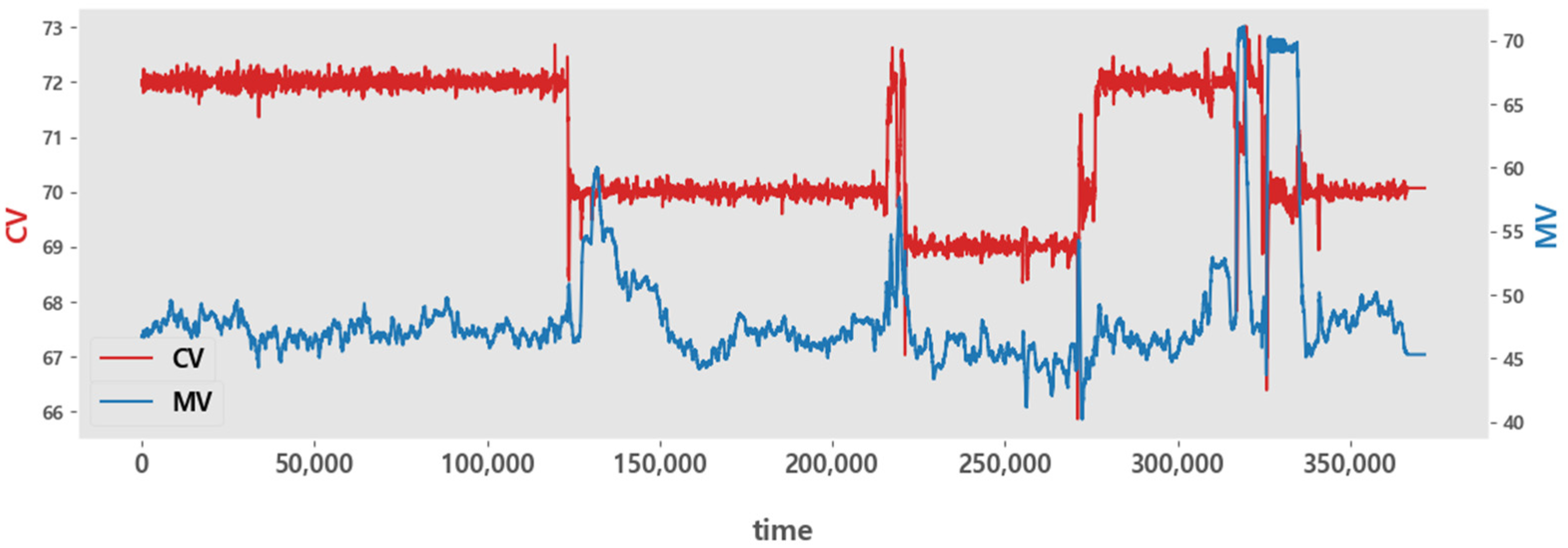
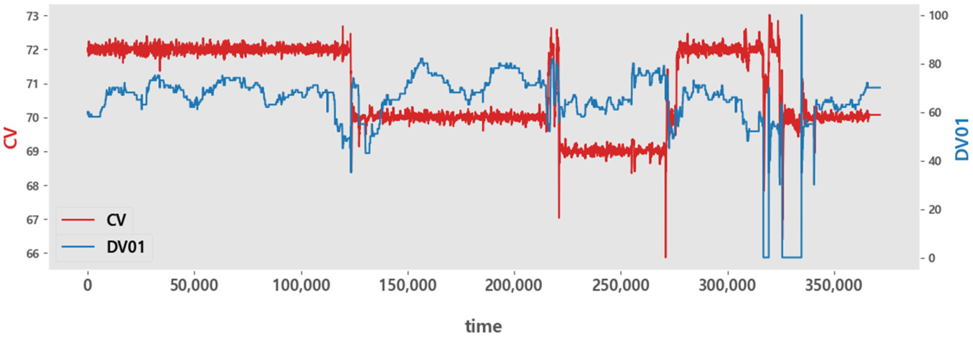
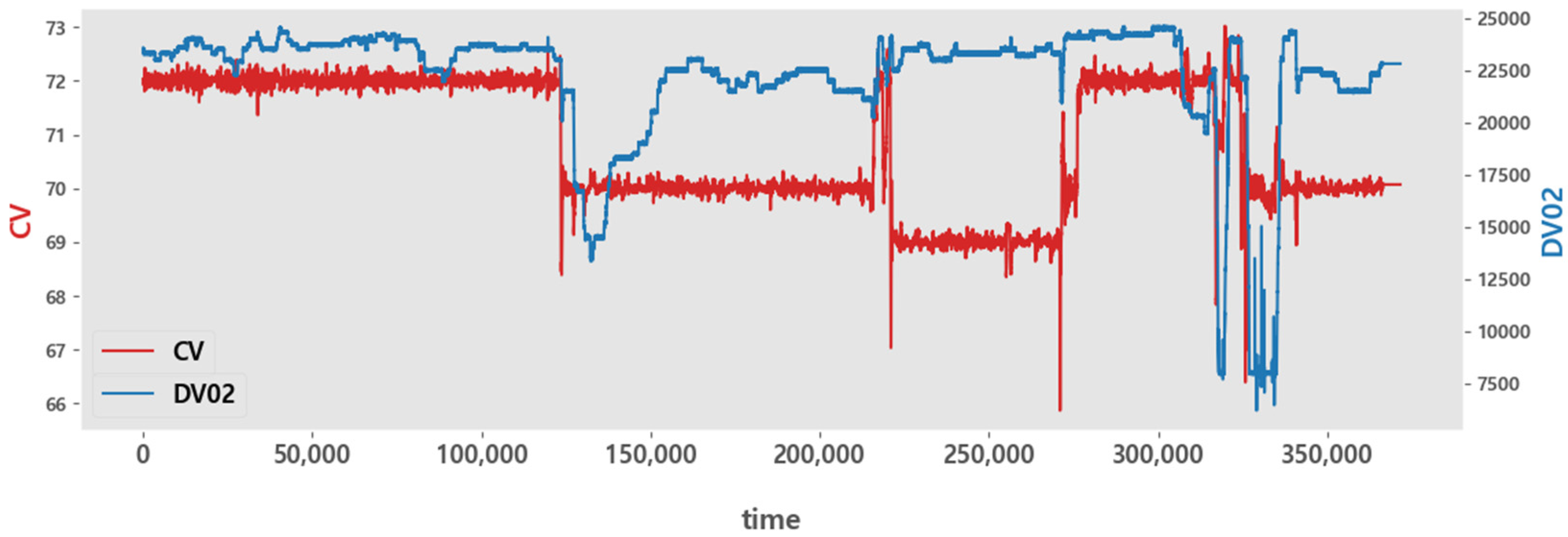
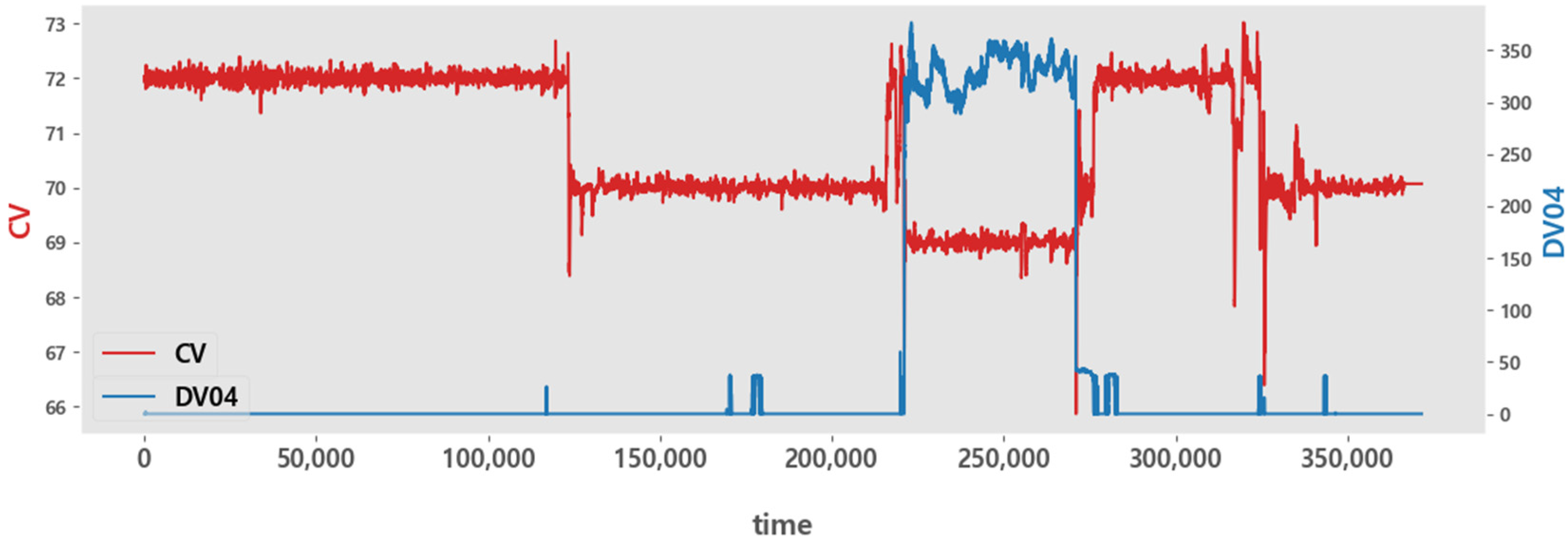
The data were collected from a real petrochemical process. We will refer to the Experiment #1 data as Plant P. The data used in Experiment #1 consist of one controlled variable, y , four disturbance variables, x , and one moderator variable, z , with 371,528 rows. For all of the independent variables, a graph visualizing their variability along with the controlled variable is shown in Figure 4. The red lines represent the controlled variables and the blue lines represent the independent variables.
Figure 4 shows the time series plots of the control and moderator variables. Figure 5, Figure 6, Figure 7 and Figure 8 show the time series plots of the controlled variables and disturbance variables. As shown in the time series plots of the controlled variables and disturbance variables, the scale of each of the control, moderator, and disturbance variables varies significantly. As a result, they were min–max normalized so that the minimum value was 0 and the maximum value was 1. This data preprocessing adjusts the scale without changing the distribution, so the relative relationship between variables is preserved and it is easy to compare or analyze various variables or features. In addition, we used the first 300,000 rows of data as training data and the last 71,528 rows of data as evaluation data. Finally, τ 1 is set to 30 and τ 2 is set to 5.

4.2.2. Experiment #2 (Plant N)

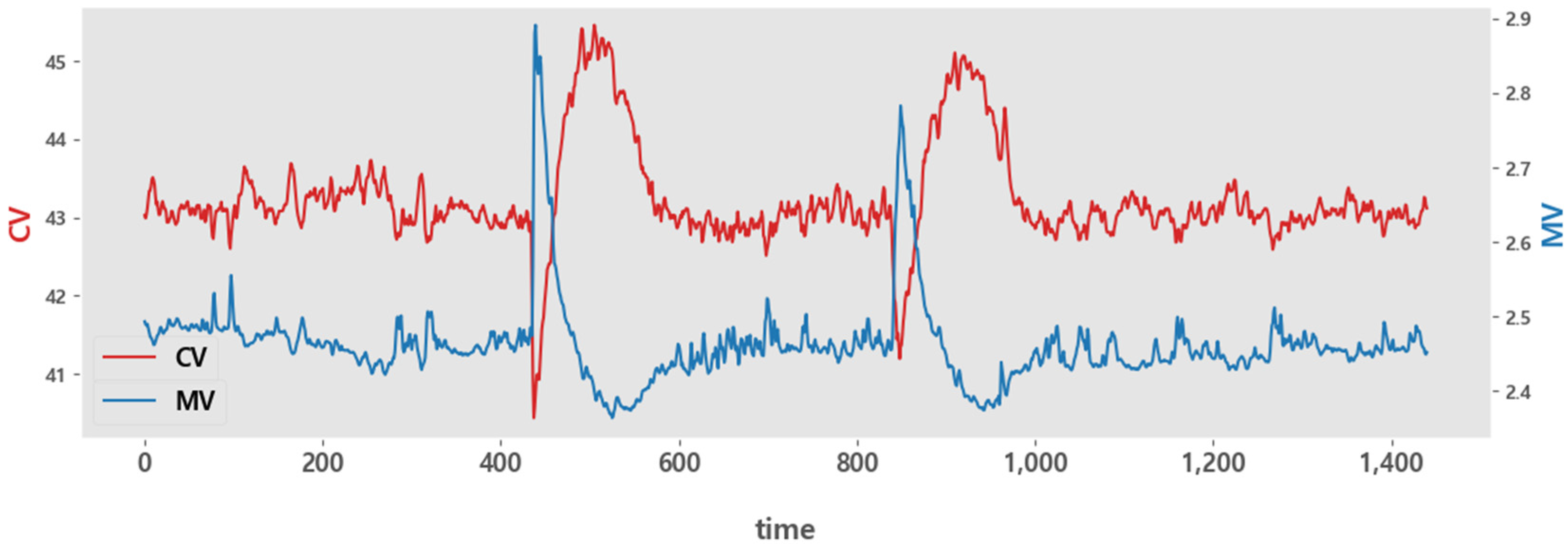
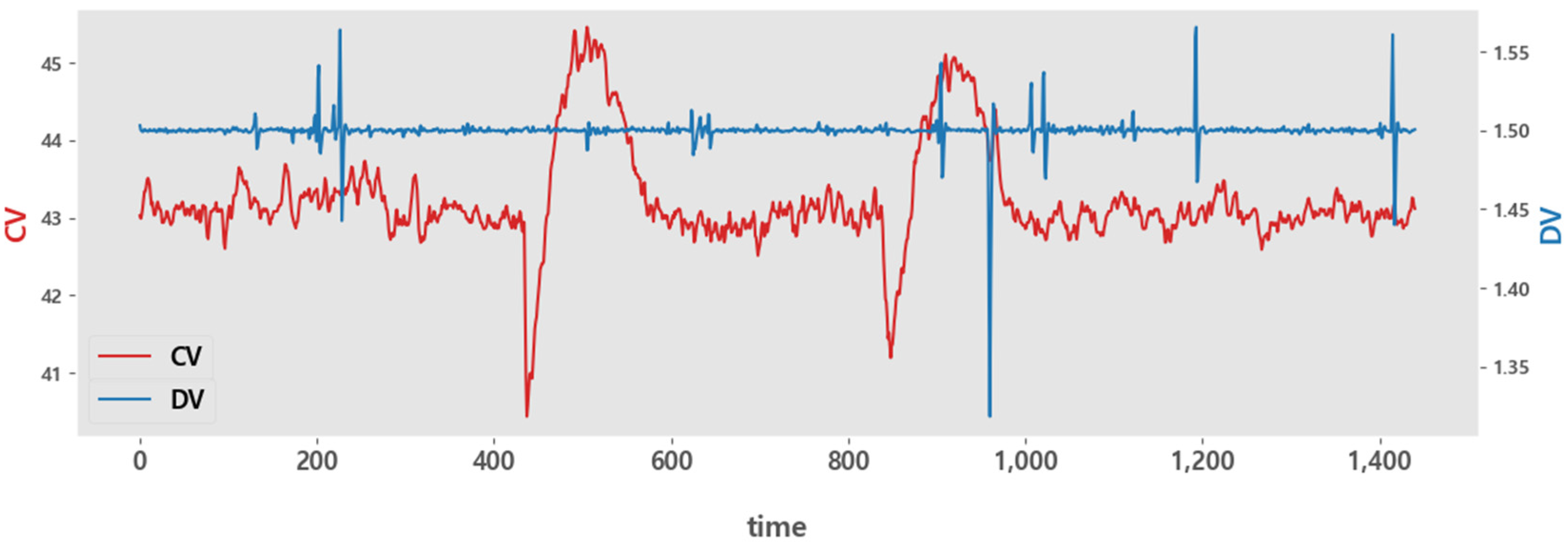
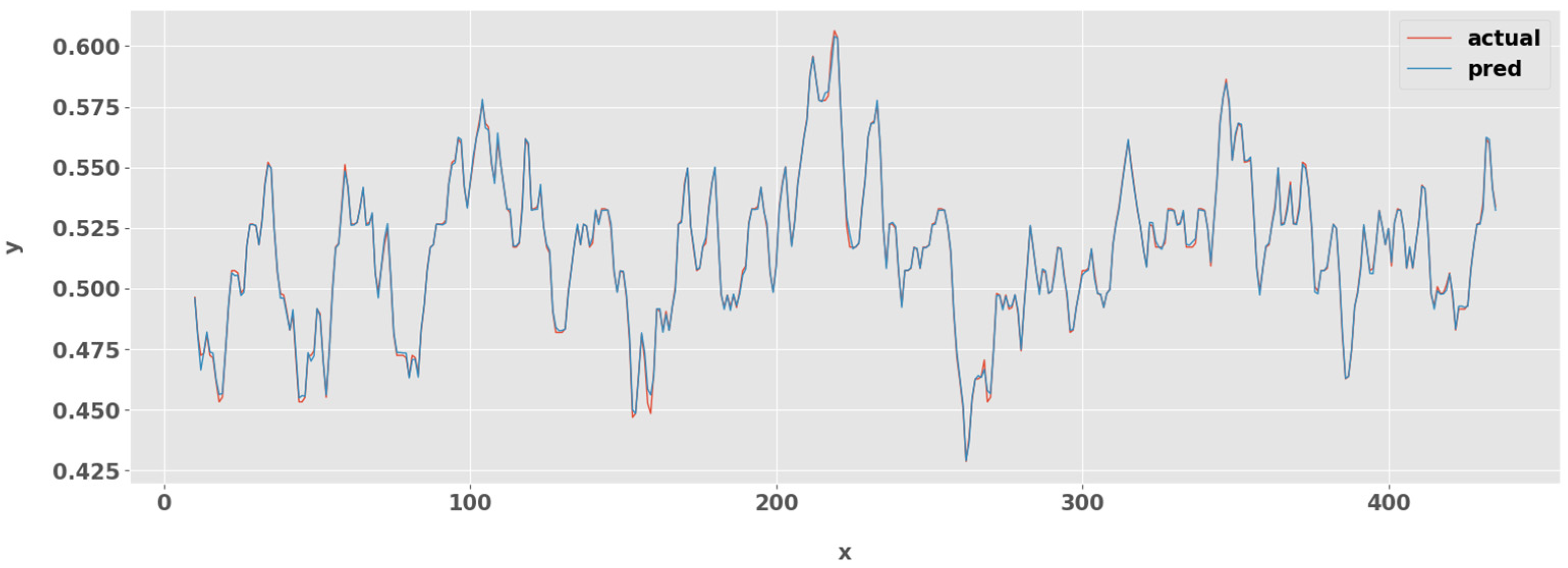
The data was collected from a real petrochemical process and the Experiment #2 data will be referred to as Plant N. The data used in this chapter consists of one controlled variable, y , one external disturbance variable, x , and one regulatory variable, z , with 1441 rows. Figure 9 and Figure 10 are graphs that visualize the variability for all independent variables, along with the controlled variables, where the red lines are the controlled variables, and the blue lines are the independent variables.
Figure 9 shows the time series plots of the control and moderator variables, and Figure 10 shows the time series plots of the control and disturbance variables. The experiment was conducted in the same way as Experiment #1, with the first 1000 rows of data as training data and the last 441 rows of data as evaluation data, with τ 1 set to 10 and τ 1 set to 5.

4.2.3. Experiment #3 (Plant S)

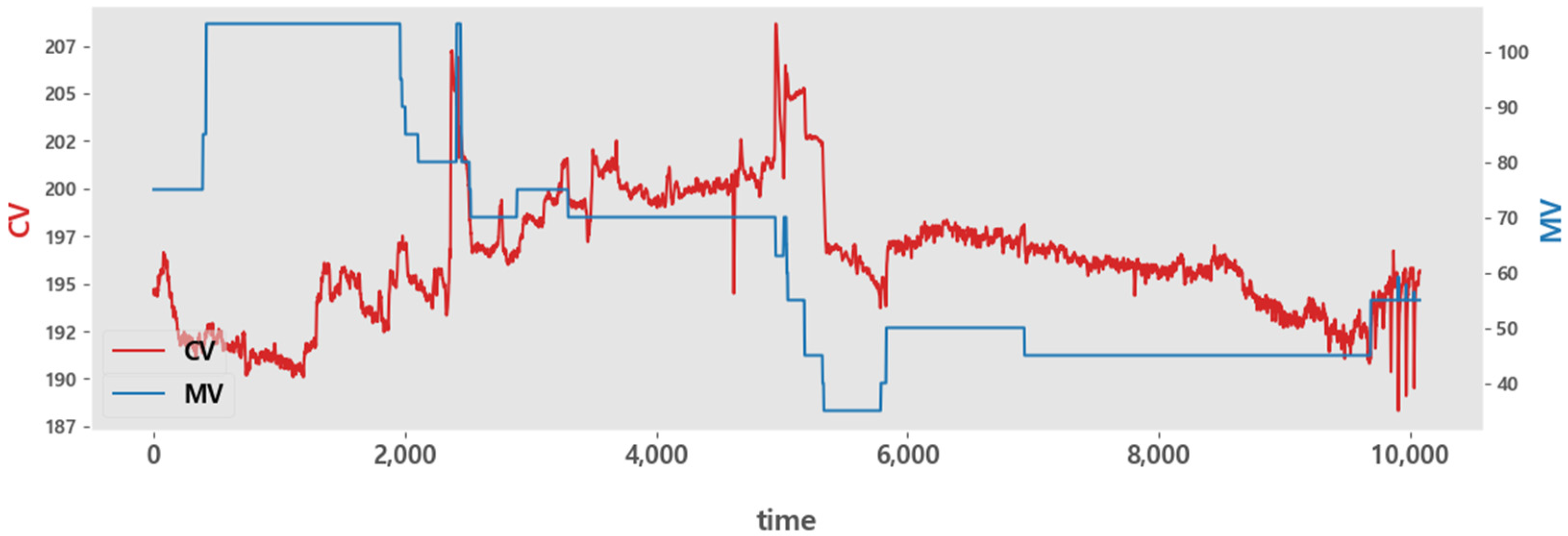
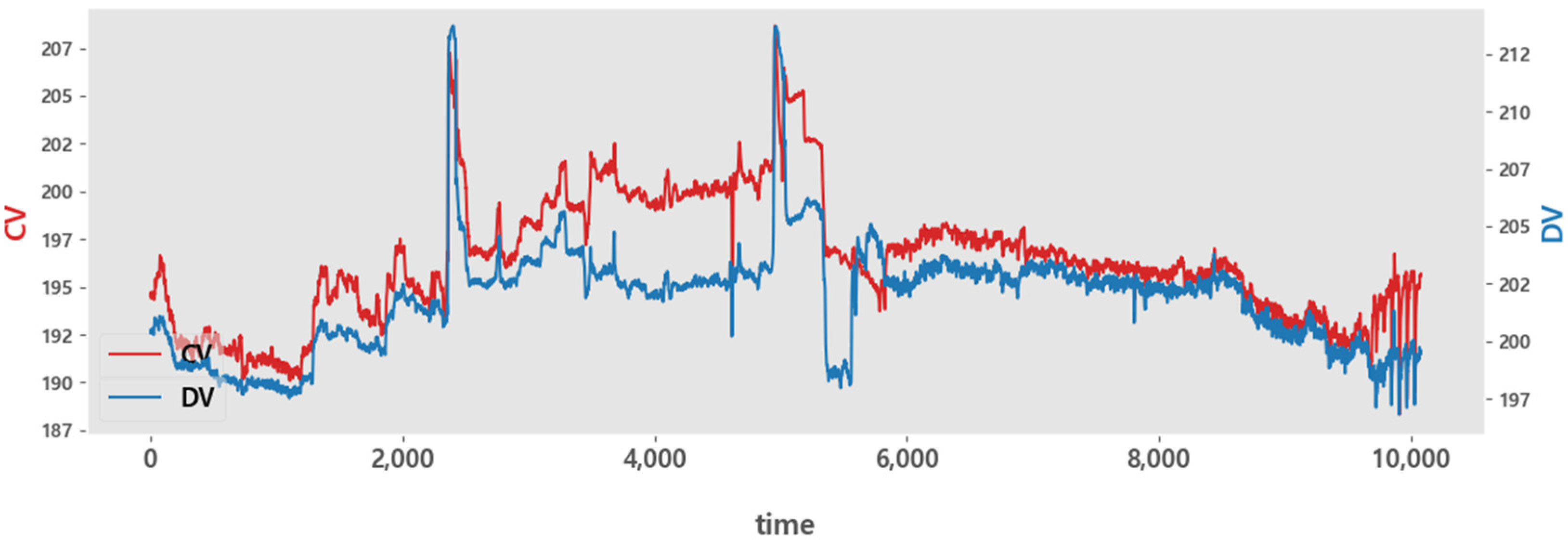
The data were collected from a real petrochemical process, and the Experiment #3 data are referred to as Plant S. The data used in this chapter consist of one controlled variable, y , one external disturbance variable, x , and one moderator variable, z , with 10,081 rows. For all independent variables, we can visualize the variability along with the controlled variable as follows. The red lines are the controlled variables, and the blue lines are the independent variables.
Figure 11 shows the time series plots of the control and moderator variables, and Figure 12 shows the time series plots of the control and disturbance variables. As shown in Figure 11 and Figure 12, the scales of each of the control, moderator, and disturbance variables are significantly different. Therefore, min–max normalization was performed so that the minimum value is 0 and the maximum value is 1. This data preprocessing adjusts the scale without changing the distribution, so it is easy to compare or analyze various variables or features while maintaining the relative relationships between variables. In addition, we used the first 7000 rows of data as training data and the last 3081 rows of data as evaluation data with set τ 1 to 10 and τ 2 to 5.

4.3. Performance Metrics

4.3.1. Mean Absolute Percentage Error (MAPE)

The mean absolute percentage error is a metric used to evaluate the accuracy of a prediction model or forecast, measuring the average percentage deviation between the predicted and actual values. It is commonly used in applications including time-series analysis, economics, and operations research [44].
MAPE = 100 n j n | e j | | A j |
  • n represents the number of observations or data points.
  • e j is the actual value of the variable you want to predict.
  • A j is the variable’s predicted value.
MAPE is expressed as a percentage, as shown in Equation (2), and represents the average size of the error between the predicted and actual values. A low MAPE indicates a more accurate prediction, while a high MAPE indicates a large difference between the predicted and actual values. MAPE is undefined when the actual value is zero. Because MAPE is an absolute percentage calculation, it gives more importance to large errors. Therefore, it is recommended to use MAPE in combination with other evaluation metrics to comprehensively evaluate the performance of a prediction model and this paper uses R2 in combination with it.

4.3.2. R-Squared

In regression analysis, the explanatory power of an independent variable is measured to explain the variability of a dependent variable. In other words, the coefficient of determination is a measure of the percentage of variability in a variable predicted by a model. A higher value indicates that the model better explains the variability of the dependent variable [45].
R 2 = 1 i = 1 n ( y i y i ^ ) 2 i = 1 n ( y i y ¯ ) 2
In Equation (3), y i is the actual value, y i is the predicted value, and y i ¯ is the average of the actual values. R2 typically has a value between 0 and 1 and can be interpreted as follows. An R2 of 1 means that the model perfectly explains the variability of the dependent variable. An R2 of 0 means that the model does not explain the variability of the dependent variable at all. When R2 is between 0 and 1, it indicates that the model explains some of the variability in the dependent variable. Higher values indicate better model explanatory power. It is important to consider the number of independent variables because R2 tends to increase automatically as the number of independent variables increases.

4.4. Results and Analysis

4.4.1. Experiment #1

A partial leaderboard of the hyper-parameter tuning results, sorted by the R2 score in descending order, is shown in Table 4:
Table 4 shows that RF performs well based on the R2 score and it can be said that it effectively predicts the controlled variables in that the R2 scores of the first through tenth-ranked models are above 0.999 and the MAPE values are below 0.245%. In addition, although the preprocessing of the data generated about 180 feature variables, the number of feature variables (k) of the top 10 best performing models tended to be in the range of about 10 to 30. The selected features, in order, are as follows.
  • Minimum value of a CV
  • Mean value of a CV
  • Maximum value of a CV
  • Maximum value of x 3
  • Previous value of x 3
From the above, we can see that the features related to the controlled variables helped to predict the controlled variables.
To determine the impact of each feature on APC’s prediction of the controlled variables, we measured the gain of the ‘Feature Importance’ attribute provided by the RF model. In Figure 13, the sum of the importance of each feature is 1:
In Figure 13, the variables that had the most impact on CV were CV_min and CV_mean. It can be concluded that these values were largely responsible for the prediction of the CV time series at the next time point. Aside from the controlled variables itself, the variable that had the greatest impact on the prediction of CV was DV03, which suggests that the previous value of DV03 influenced the current value of CV in a staggered manner. Figure 14 shows the average R2 for each model.
In Figure 14, XGB, RF, and NN perform well with R2 scores close to 1.0. Considering the R2 score, we can see that all the models are quite effective in predicting Plant P. This is because the data of Plant P consists of many independent variables and the long time-series data can be trained to explain the controlled variables sufficiently.
Figure 15 is a graph depicting the results of predicting the controlled variables based on the best performing models.
In Figure 15, we can see that the predicted values are not significantly different from the actual values. Plant P has the most data compared to the other plants, so it is the best trained and has an R2 score of 0.99949, which is close to 1, which means it perfectly explains the variability of the dependent variable. The MAPE score is 0.228, which means that the average size of the error between the predicted value and the actual value is small, and it makes accurate predictions. The highest number of disturbance variables is presumably the reason for the best prediction.

4.4.2. Experiment #2

Table 5 shows some of the hyper-parameter tuning results, sorted in descending order based on the R2 score:
Table 5 shows that RF outperforms the other models based on its R2 score, but it does not appear to be significantly different from XGB’s R2 score, which is shown in the top 2 through 9 results. The highest performing model is the RF model, but the overall model performance (average) is the highest for XGB. In Table 5, the top 10 models all have an R2 score of 0.997 or higher and a MAPE value of 0.195% or less, indicating that they effectively predict the controlled variables.
  • Minimum value of CV
  • Mean value of CV
  • Maximum value of CV
  • Previous value of x
  • Standard deviation of CV
  • Standard deviation of x
  • Average amount of change of x
  • Mean value of x
  • Maximum value of x
From the above, we can see that the features related to the controlled variable helped predict the controlled variable.
To determine the impact of each feature on APC’s prediction of the controlled variable, we measured the gain of the ‘Feature Importance’ attribute provided by the RF model. In Figure 16, the sum of the importance of each feature is 1:
In Figure 16, CV_min and CV_mean are the variables that have the most influence on CV, and the values of these variables are used to predict the CV time series at the next time point. In addition to the variables related to CV, we can see that DV has the largest impact. It is determined that the previous value of DV has affected the current value of CV with a time lag.
Figure 17 shows the average R2 score, sorted by model:
In Figure 17, the RF and XGB models have noticeably higher R2 scores. Consistent with the previous results, we see that the XGB model has the highest R2 score on average.
Figure 18 plots the results of predicting the controlled variables based on the best performing models:
In Figure 18, we can see that Plant N has a high prediction accuracy, just like Plant P. The RF model, which is selected as the best model, has an R2 score of 0.9972 and a MAPE of 0.1941%, which means that the model can fully explain the variability of the dependent variable.

4.4.3. Experiment #3

Some of the hyper-parameter tuning results, sorted by R2 score in descending order, are shown in Table 6.
Table 6 shows that the NN, SVR, and XGB models perform well based on their R2 scores. As in Experiment #1, the NN model performs the best and the XGB model is stable regardless of the parameters.
When the model performance is listed in terms of R2, all the models in Table 6 have an R2 score of 0.959 or higher and a MAPE of 9.76% or less, indicating that they effectively predict the controlled variables. The selected features, in order, are as follows.
  • Minimum value of CV
  • Minimum value of x
  • Previous value of z = z t ,   ,   z t τ 1
  • Minimum value of z
  • Previous value of x = x t ,   ,   x t τ 1
  • Mean value of x
  • Maximum value of z
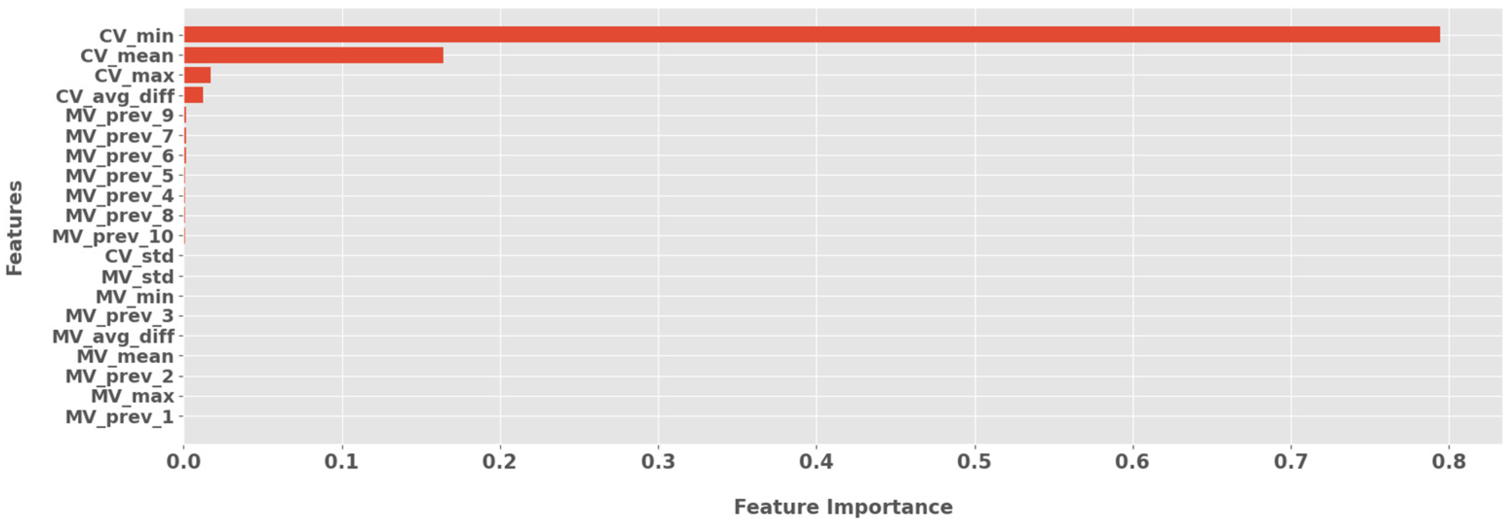
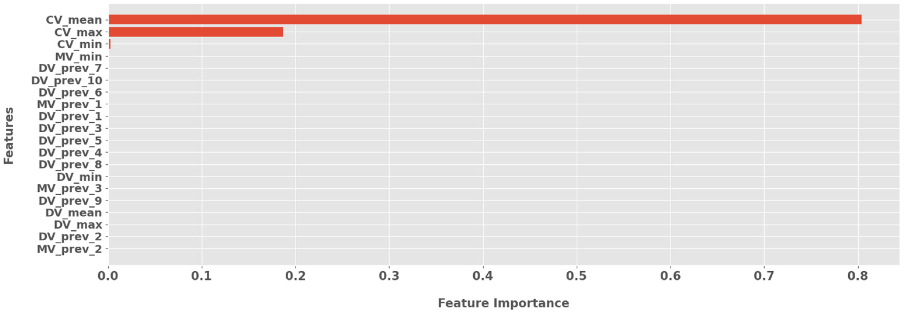
From the above, we can see that the features related to the CV helped predict the CV. To determine the impact of each feature on APC’s prediction of CV, we measured the gain of the ‘Feature Importance’ attribute provided by the RF model. In Figure 19, the sum of the importance of each feature is 1:
In Figure 19, the variables that had the most impact on CV were CV_mean and CV_max, and these values were largely responsible for predicting the CV time-series at the next point in time.
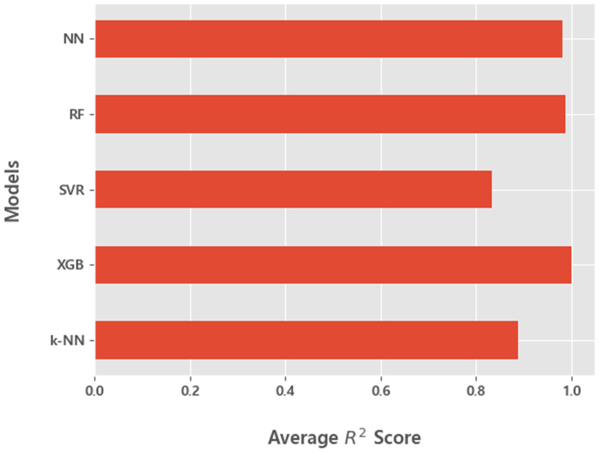
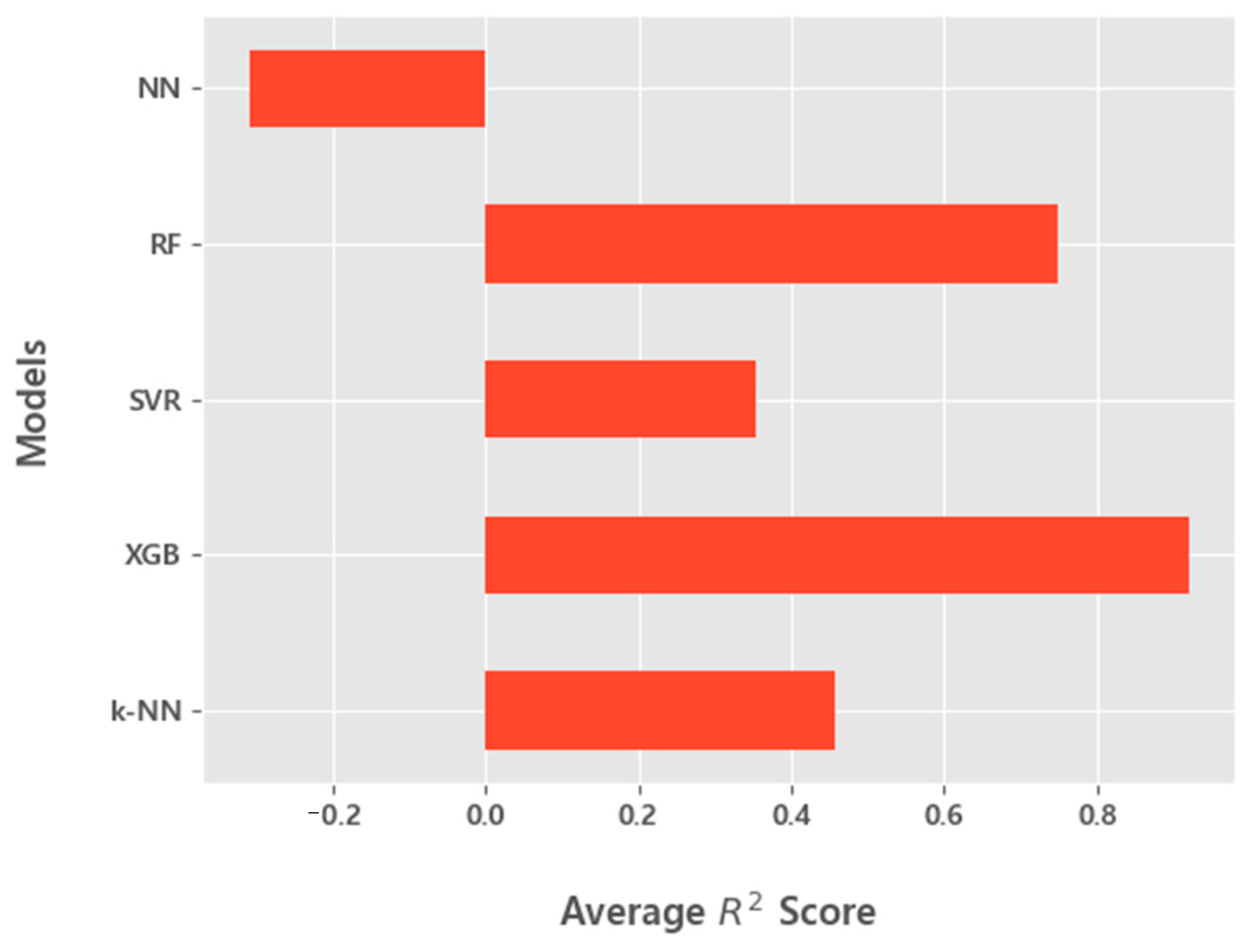
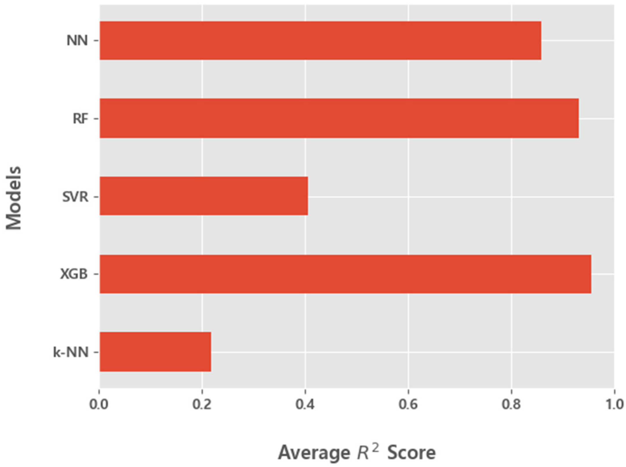
Figure 20 shows the average R2 score per model:
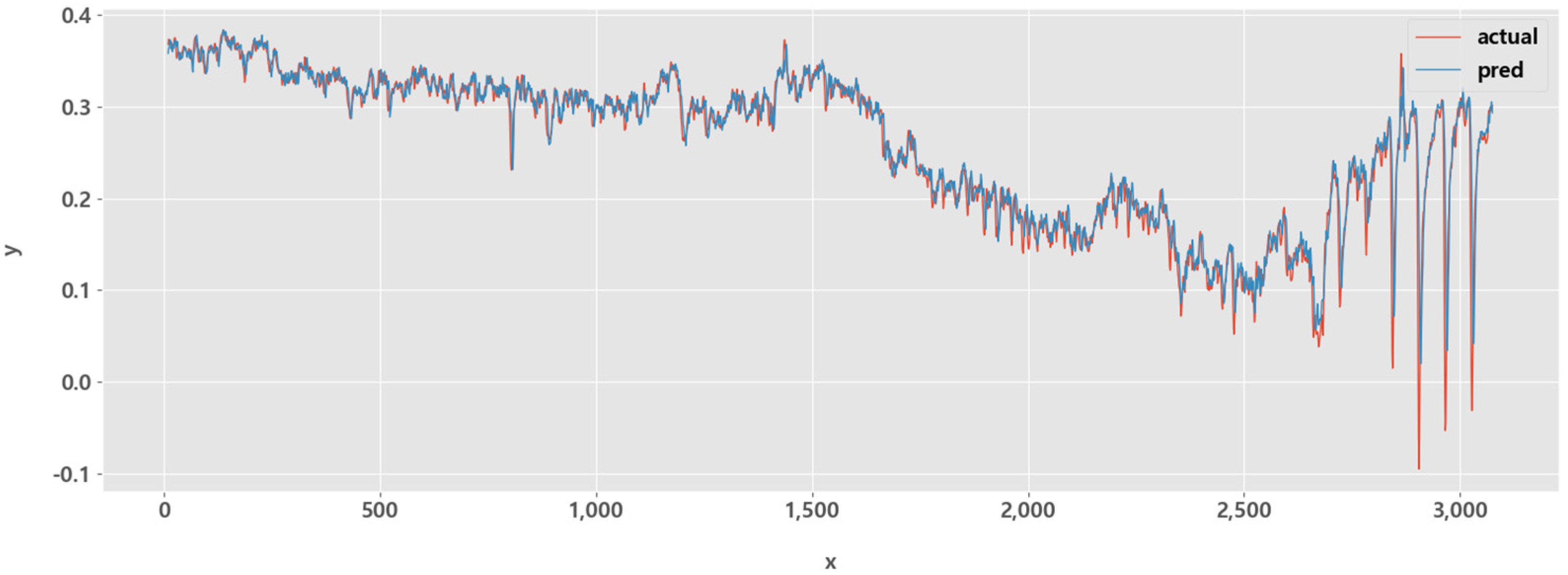
In Figure 20, XGB has the highest R2 score, followed by the RF model and then the NN model. Figure 21 shows the prediction of the controlled variables based on the best performing model:
In Figure 21, we can see that Plant S has a larger MAPE value than Plant P and Plant N, so the predicted data do not follow the actual data in some bins, but the overall trend is well followed. The model is especially significant in that it predicts large fluctuations in the 2500–3000 range with high accuracy. The MAPE values of the top 10 models are between 6.0% and 9.0%, which is high compared to the other plants, but the explanatory power of the models can be judged to be sufficiently significant given the large fluctuations in controlled variables in the second half of the test data and the high R2 scores of the top models.

5. Conclusions

This study demonstrates the feasibility of using machine learning models to predict control variables for the adoption of APC systems in the petrochemical industry. In an APC system, the prediction of control variables and how the control variable values are modified to be within the user’s desired range are of utmost importance. This study mainly focused on the prediction of control variables and utilized various machine learning techniques to predict future control variables based on past control variables, manipulated variables, and external disturbance variables. By using time delay as a parameter and adjusting its value, we were able to analyze the relationship between past and future data and improve the prediction performance. Currently, APC systems are controlled through mathematical modeling, and research is trending toward predicting time series data of control variables, manipulation variables, and external disturbance variables with machine learning models to compare performance and measure accuracy. It is becoming increasingly important to change from mathematical prediction models to data-driven machine learning predictions. The results of R-squared (R2) and Mean Absolute Percentage Error (MAPE) metrics in this study demonstrate the feasibility of introducing machine learning models into APC systems in petrochemical plants.
This paper presents two directions for future research. First, to further improve the performance of APC’s controlled variables prediction, the performance should be evaluated against machine learning models. It should be investigated whether other ensemble methods such as LightGBM or machine learning algorithms can be applied to further improve the controlled variables prediction performance. Second, research should be conducted to determine the optimal controlled variables values. In the aforementioned APC system, the most important aspect is the optimal MV for CV prediction and CV control. We propose to determine the optimal MV through machine learning. Additionally, upon completion of the research, it is necessary to develop a linear dynamic model and compare it with real data to enhance its completeness. To this end, this paper is the first step in exploring the possibility of predicting and controlling controlled variables of APC systems in petrochemical plants through machine learning, which opens new possibilities for improving the efficiency and performance of automatic control in the petrochemical industry.

Author Contributions

Conceptualization, M.L. and Y.Y.; validation, M.L., Y.Y., C.L. and J.J.; formal analysis, Y.C. and S.B.; investigation, Y.C., S.B., Y.K., H.J., D.L. and K.K.; methodology, M.L.; software, M.L., Y.Y. and H.B.; data curation, J.J.; original draft preparation, M.L.; review and editing, M.L., Y.Y. and J.J.; funding acquisition, J.J. All authors have read and agreed to the published version of the manuscript.

Funding

This research was supported by the SungKyunKwan University and the BK21 FOUR (Graduate School Innovation) and funded by the Ministry of Education (MOE, Korea) and National Research Foundation of Korea (NRF).

Data Availability Statement

The data used to support the findings of this study will be provided by the corresponding author upon request ([email protected]).

Acknowledgments

This research was supported by the SungKyunKwan University and the BK21 FOUR (Graduate School Innovation) and funded by the Ministry of Education (MOE, Korea) and National Research Foundation of Korea (NRF). Moreover, this research was supported by the MSIT (Ministry of Science and ICT), Korea, under the ITRC (Information Technology Research Center) support program (IITP-2023-2018-0-01417) and supervised by the IITP (Institute for Information & Communications Technology Planning & Evaluation).

Conflicts of Interest

The authors declare no conflict of interest.

References

  1. Seborg, D.E. Automation and control of chemical and petrochemical plants. In Control Systems, Robotics and Automation; Eolss: Oxford, UK, 2009; p. 496. [Google Scholar]
  2. Proctor, L.; Dunn, P.J.; Hawkins, J.M.; Wells, A.S.; Williams, M.T. Continuous processing in the pharmaceutical industry. In Green Chemistry in the Pharmaceutical Industry; Wiley-VCH Verlag GmbH & Co. KGaA: Weinheim, Germany, 2010; pp. 221–242. [Google Scholar]
  3. Li, Y.; Ang, K.H.; Chong, G.C. PID control system analysis and design. IEEE Control Syst. Mag. 2006, 26, 32–41. [Google Scholar]
  4. Xinping, Z.; Quanshan, L.; Huan, W.; Wenxin, W.; Qibing, J.; Lideng, P. The application of model PID or IMC-PID advanced process control to refinery and petrochemical plants. In Proceedings of the 2007 Chinese Control Conference, Zhangjiajie, China, 26–31 July 2007; IEEE: Piscataway, NJ, USA; pp. 699–703. [Google Scholar]
  5. Qin, S.J.; Badgwell, T.A. An overview of industrial model predictive control technology. In AIche Symposium Series; 1971-c2002; American Institute of Chemical Engineers: New York, NY, USA, 1997; Volume 93, pp. 232–256. [Google Scholar]
  6. Clavijo, N.; Melo, A.; Câmara, M.M.; Feital, T.; Anzai, T.K.; Diehl, F.C.; Thompson, P.H.; Pinto, J.C. Development and Application of a Data-Driven System for Sensor Fault Diagnosis in an Oil Processing Plant. Processes 2019, 7, 436. [Google Scholar] [CrossRef] [Green Version]
  7. Xiang, S.; Bai, Y.; Zhao, J. Medium-term prediction of key chemical process parameter trend with small data. Chem. Eng. Sci. 2022, 249, 117361. [Google Scholar] [CrossRef]
  8. Diehl, F.C.; Machado, T.O.; Anzai, T.K.; Almeida, C.S.; Moreira, C.A.; Nery Jr, G.A.; Campos, M.C.; Farenzena, M.; Trierweiler, J.O. 10% increase in oil production through a field applied APC in a Petrobras ultra-deepwater well. Control Eng. Pract. 2019, 91, 104108. [Google Scholar] [CrossRef]
  9. Lababidi, H.M.; Kotob, S.; Yousuf, B. Refinery advanced process control planning system. Comput. Chem. Eng. 2002, 26, 1303–1319. [Google Scholar] [CrossRef]
  10. Moro, L.F.L. Process technology in the petroleum refining industry—Current situation and future trends. Comput. Chem. Eng. 2003, 27, 1303–1305. [Google Scholar] [CrossRef]
  11. Haque, M.E.; Palanki, S.; Xu, Q. Advanced Process Control for Cost-Effective Glycol Loss Minimization in a Natural Gas Dehydration Plant under Upset Conditions. Ind. Eng. Chem. Res. 2020, 59, 7680–7692. [Google Scholar] [CrossRef]
  12. Serale, G.; Fiorentini, M.; Capozzoli, A.; Bernardini, D.; Bemporad, A. Model predictive control (MPC) for enhancing building and HVAC system energy efficiency: Problem formulation, applications and opportunities. Energies 2018, 11, 631. [Google Scholar] [CrossRef] [Green Version]
  13. Afram, A.; Janabi-Sharifi, F. Theory and applications of HVAC control systems–A review of model predictive control (MPC). Build. Environ. 2014, 72, 343–355. [Google Scholar] [CrossRef]
  14. Killian, M.; Kozek, M. Ten questions concerning model predictive control for energy efficient buildings. Build. Environ. 2016, 105, 403–412. [Google Scholar] [CrossRef]
  15. Barrera-Animas, A.Y.; Oyedele, L.O.; Bilal, M.; Akinosho, T.D.; Delgado, J.M.D.; Akanbi, L.A. Rainfall prediction: A comparative analysis of modern machine learning algorithms for time-series forecasting. Mach. Learn. Appl. 2022, 7, 100204. [Google Scholar] [CrossRef]
  16. Khosravi, A.; Machado, L.; Nunes, R.O. Time-series prediction of wind speed using machine learning algorithms: A case study Osorio wind farm, Brazil. Appl. Energy 2018, 224, 550–566. [Google Scholar] [CrossRef]
  17. Mudelsee, M. Trend analysis of climate time series: A review of methods. Earth-Sci. Rev. 2019, 190, 310–322. [Google Scholar] [CrossRef]
  18. Lu, C.J.; Lee, T.S.; Chiu, C.C. Financial time series forecasting using independent component analysis and support vector regression. Decis. Support Syst. 2009, 47, 115–125. [Google Scholar] [CrossRef]
  19. Parray, I.R.; Khurana, S.S.; Kumar, M.; Altalbe, A.A. Time series data analysis of stock price movement using machine learning techniques. Soft Comput. 2020, 24, 16509–16517. [Google Scholar] [CrossRef]
  20. Sagheer, A.; Kotb, M. Time series forecasting of petroleum production using deep LSTM recurrent networks. Neurocomputing 2019, 323, 203–213. [Google Scholar] [CrossRef]
  21. Kwon, H.; Oh, K.C.; Choi, Y.; Chung, Y.G.; Kim, J. Development and application of machine learning-based prediction model for distillation column. Int. J. Intell. Syst. 2021, 36, 1970–1997. [Google Scholar] [CrossRef]
  22. Han, Y.; Zeng, Q.; Geng, Z.; Zhu, Q. Energy management and optimization modeling based on a novel fuzzy extreme learning machine: Case study of complex petrochemical industries. Energy Convers. Manag. 2018, 165, 163–171. [Google Scholar] [CrossRef]
  23. Geng, Z.; Zhang, Y.; Li, C.; Han, Y.; Cui, Y.; Yu, B. Energy optimization and prediction modeling of petrochemical industries: An improved convolutional neural network based on cross-feature. Energy 2020, 194, 116851. [Google Scholar] [CrossRef]
  24. Oleander, T. Machine Learning Framework for Petrochemical Process Industry Applications. Available online: https://aaltodoc.aalto.fi/handle/123456789/35514 (accessed on 12 June 2023).
  25. Raó, W. Advanced Process Control; McGraw-Hill: New York, NY, USA, 1981. [Google Scholar]
  26. Su, H.T. Operation-oriented advanced process control. In Proceedings of the 2004 IEEE International Symposium on Intelligent Control, Taipei, Taiwan, 4 September 2004; IEEE: Piscataway, NJ, USA; pp. 252–257. [Google Scholar]
  27. Mayne, D.Q. Model predictive control: Recent developments and future promise. Automatica 2014, 50, 2967–2986. [Google Scholar] [CrossRef]
  28. Morari, M.; Lee, J.H. Model predictive control: Past, present and future. Comput. Chem. Eng. 1999, 23, 667–682. [Google Scholar] [CrossRef]
  29. Qin, S.J.; Badgwell, T.A. A survey of industrial model predictive control technology. Control Eng. Pract. 2003, 11, 733–764. [Google Scholar] [CrossRef]
  30. Rodriguez-Galiano, V.; Sanchez-Castillo, M.; Chica-Olmo, M.; Chica-Rivas, M.J.O.G.R. Machine learning predictive models for mineral prospectivity: An evaluation of neural networks, random forest, regression trees and support vector machines. Ore Geol. Rev. 2015, 71, 804–818. [Google Scholar] [CrossRef]
  31. Breiman, L. Random forests. Mach. Learn. 2001, 45, 5–32. [Google Scholar] [CrossRef] [Green Version]
  32. Masini, R.P.; Medeiros, M.C.; Mendes, E.F. Machine learning advances for time series forecasting. J. Econ. Surv. 2023, 37, 76–111. [Google Scholar] [CrossRef]
  33. Tyralis, H.; Papacharalampous, G. Variable selection in time series forecasting using random forests. Algorithms 2017, 10, 114. [Google Scholar] [CrossRef] [Green Version]
  34. Noble, W.S. What is a support vector machine? Nat. Biotechnol. 2006, 24, 1565–1567. [Google Scholar] [CrossRef]
  35. Awad, M.; Khanna, R. Efficient Learning Machines: Theories, Concepts, and Applications for Engineers and System Designers; Springer Nature: Berlin, Germany, 2015; p. 268. [Google Scholar]
  36. Abiodun, O.I.; Jantan, A.; Omolara, A.E.; Dada, K.V.; Mohamed, N.A.; Arshad, H. State-of-the-art in artificial neural network applications: A survey. Heliyon 2018, 4, e00938. [Google Scholar] [CrossRef] [Green Version]
  37. Martínez, F.; Frías, M.P.; Pérez, M.D.; Rivera, A.J. A methodology for applying k-nearest neighbor to time series forecasting. Artif. Intell. Rev. 2019, 52, 2019–2037. [Google Scholar] [CrossRef]
  38. Chen, T.; Guestrin, C. Xgboost: A scalable tree boosting system. In Proceedings of the 22nd Acm Sigkdd International Conference on Knowledge Discovery and Data Mining, San Francisco, CA, USA, 13–17 August 2016; pp. 785–794. [Google Scholar]
  39. Wuest, T.; Weimer, D.; Irgens, C.; Thoben, K.D. Machine learning in manufacturing: Advantages, challenges, and applications. Prod. Manuf. Res. 2016, 4, 23–45. [Google Scholar] [CrossRef] [Green Version]
  40. Parmezan, A.R.S.; Souza, V.M.; Batista, G.E. Evaluation of statistical and machine learning models for time series prediction: Identifying the state-of-the-art and the best conditions for the use of each model. Inf. Sci. 2019, 484, 302–337. [Google Scholar] [CrossRef]
  41. Shi, J.; Jain, M.; Narasimhan, G. Time series forecasting (tsf) using various deep learning models. arXiv 2022, arXiv:2204.11115. [Google Scholar]
  42. Box, G.E.; Jenkins, G.M.; Reinsel, G.C.; Ljung, G.M. Time Series Analysis: Forecasting and Control; John Wiley & Sons: Hoboken, NJ, USA, 2015. [Google Scholar]
  43. Paine, T.L.; Paduraru, C.; Michi, A.; Gulcehre, C.; Zolna, K.; Novikov, A.; Wang, Z.; de Freitas, N. Hyperparameter selection for offline reinforcement learning. arXiv 2020, arXiv:2007.09055. [Google Scholar]
  44. Botchkarev, A. A new typology design of performance metrics to measure errors in machine learning regression algorithms. Interdiscip. J. Inf. Knowl. Manag. 2019, 14, 045–076. [Google Scholar] [CrossRef] [PubMed] [Green Version]
  45. Catal, C. Performance evaluation metrics for software fault prediction studies. Acta Polytech. Hung. 2012, 9, 193–206. [Google Scholar]
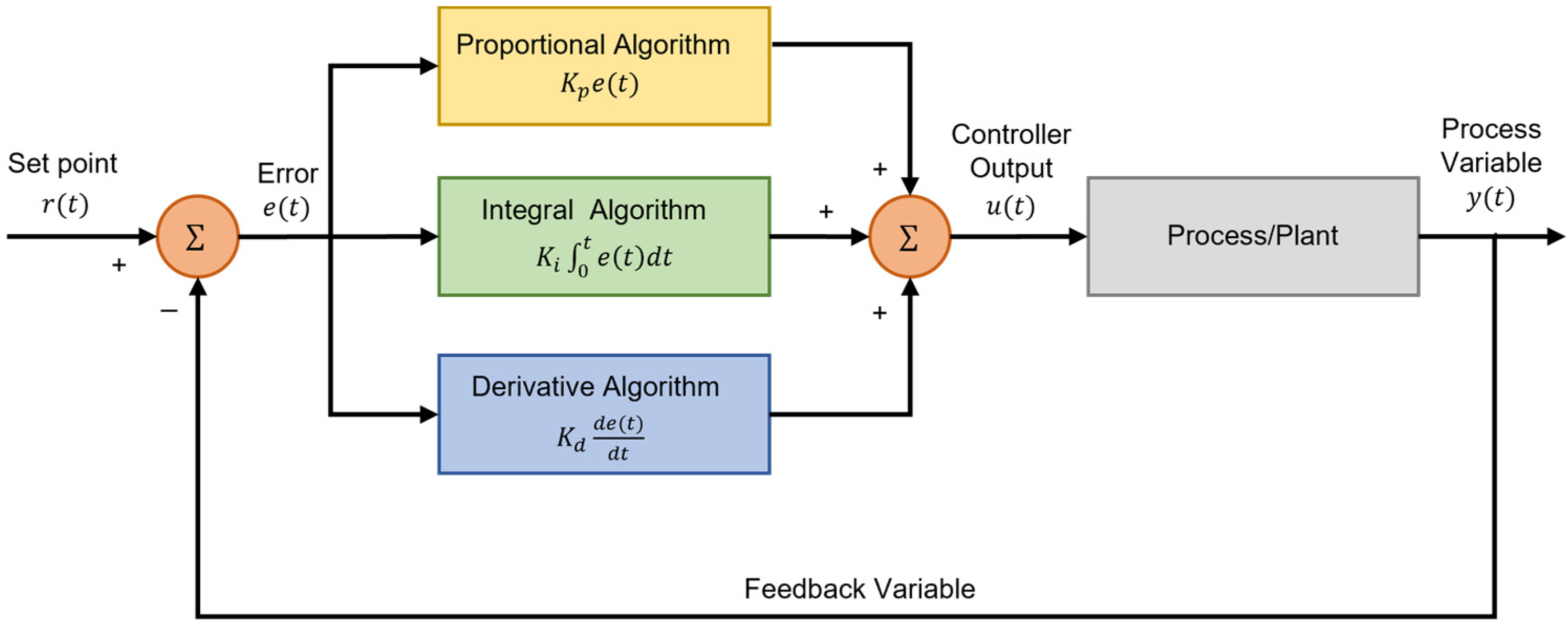
Figure 1. Block Diagram of PID Controller.
Processes 11 02091 g001
Figure 2. Block diagram of APC Controller.
Processes 11 02091 g002
Figure 3. Overall architecture.
Processes 11 02091 g003
Figure 4. Time series plots of the CV and MV in Plant P.
Processes 11 02091 g004
Figure 5. Time series plots of the CV and first external DV in Plant P.
Processes 11 02091 g005
Figure 6. Time series plots of the CV and second external DV in Plant P.
Processes 11 02091 g006
Figure 7. Time series plots of the CV and third external DV in Plant P.
Processes 11 02091 g007
Figure 8. Time series plots of the CV and fourth external DV in Plant P.
Processes 11 02091 g008
Figure 9. Time series plots of the CV and MV in Plant N.
Processes 11 02091 g009
Figure 10. Time series plots of the CV and external DV in Plant N.
Processes 11 02091 g010
Figure 11. Time series plots of the CV and MV in Plant S.
Processes 11 02091 g011
Figure 12. Time series plots of the CV and external DV in Plant S.
Processes 11 02091 g012
Figure 13. Plant P feature importance plot.
Processes 11 02091 g013
Figure 14. Average R2 score per model in Plant P.
Processes 11 02091 g014
Figure 15. Visualization of the prediction results in Plant P.
Processes 11 02091 g015
Figure 16. Plant N feature importance plot.
Processes 11 02091 g016
Figure 17. Average R2 score per model in Plant N.
Processes 11 02091 g017
Figure 18. Visualization of the prediction results in Plant N.
Processes 11 02091 g018
Figure 19. Plant S feature importance plot.
Processes 11 02091 g019
Figure 20. Average R2 score per model in Plant S.
Processes 11 02091 g020
Figure 21. Visualization of the prediction results in Plant S.
Processes 11 02091 g021
Table 1. Features sets considered.
FeatureEquation for Variable x
Mean m = i = 1 n x i n
Standard deviation s t d = i = 1 n ( x i m ) n 2
Skew s k e w = 1 n × i = 1 n ( x i m ) 3 s t d 3
Kurt k u r t = 1 n × i = 1 n ( x i m ) 4 s t d 4
Maximum max ( x 1 , x 2 , x n )
Minimum min ( x 1 , x 2 , x n )
Average Change 1 n i = 0 n 1 ( x i + 1 x i )
Table 2. Machine learning models and hyper-parameter grid.
Machine Learning ModelHyper-Parameter Grid
Neural Network (NN)• Maximum iterations: 10,000
• Active function: ReLU
• Hidden layers: {(10), (10, 10), (10, 10, 10), (10, 10, 10, 10)}
Support Vector Regression (SVR)• Maximum iterations: 10,000
• Kernel: {rbf, linear}
• Penalty Factors: {0.1, 1, 10}
Random Forest (RF)• Decision Tree max depths: {3, 5, 7, 9}
• Percentage of features when branching: {0.6, 0.8, 1.0}
k-Nearest Neighbor (k-NN)• Neighbor numbers: {3, 5, 7, 9}
XGBoost (XGB)• Learning rates: {0.05, 0.1, 0.15, 0.2}
• Decision Tree max depths: {3, 5, 7, 9}
• Number of Decision Trees: {200, 400, 600, 800}
Table 3. Hardware Platform Specifications.
Laptop ConfigurationSpecification
CPUCore i5—8250
RAM8GB RAM
Operating SystemWindow 10
Table 4. Results of hyper-parameter tuning.
RankModelParameterKR2MAPE
1RFMax Depth: 9
Feature Percentage: 0.8
100.999490.228
2RFMax Depth: 9
Feature Percentage: 1.0
100.999490.2299
3RFMax Depth: 7
Feature Percentage: 0.8
100.999470.2281
4RFMax Depth: 7
Feature Percentage: 1.0
100.999470.2304
5XGBLearning Rate: 0.05
Max Depth: 3 Number of decision trees: 400
100.999470.2376
6XGBLearning Rate: 0.05
Max Depth: 3 Number of decision trees: 400
300.999470.2437
7RFMax Depth: 7
Feature Percentage: 1.0
300.999470.2309
8XGBLearning Rate: 0.05
Max Depth: 3 Number of decision trees: 400
200.999460.2434
9XGBLearning Rate: 0.05
Max Depth: 3 Number of decision trees: 600
100.999460.2421
10RFMax Depth: 7
Feature Percentage: 0.8
300.999460.2303
Table 5. Results of hyper-parameter tuning.
RankModelParameterKR2MAPE
1RFMax Depth: 9
Feature Percentage: 1.0
200.997620.1941
2XGBLearning Rate: 0.1
Max Depth: 7
Number of decision trees: 400
200.997620.1844
3XGBLearning Rate: 0.1
Max Depth: 7
Number of decision trees: 800
200.997620.1844
4XGBLearning Rate: 0.1
Max Depth: 7
Number of decision trees: 600
200.997620.1844
5XGBLearning Rate: 0.05
Max Depth: 7
Number of decision trees: 600
300.997610.18
6XGBLearning Rate: 0.05
Max Depth: 7
Number of decision trees: 800
300.997610.18
7XGBLearning Rate: 0.05
Max Depth: 7
Number of decision trees: 400
300.997610.18
8XGBLearning Rate: 0.05
Max Depth: 7
Number of decision trees: 200
300.997610.18
9XGBLearning Rate: 0.1
Max Depth: 7
Number of decision trees: 200
200.99760.1852
10XGBLearning Rate: 0.05
Max Depth: 9
Number of decision trees: 600
300.997590.1593
Table 6. Results of hyper-parameter tuning.
RankModelParameterKR2MAPE
1NNHidden layer: (10,)200.967299.0095
2NNHidden layer: (10, 10)200.964727.5151
3NNHidden layer: (10, 10, 10, 10)100.964576.0797
4XGBLearning Rate: 0.15
Max Depth: 3
Number of decision trees: 800
200.961048.0518
5SVRC: 1, Kernel: Linear100.960859.7507
6XGBLearning Rate: 0.15
Max Depth: 3
Number of decision trees: 600
200.960358.1201
7XGBLearning Rate: 0.15
Max Depth: 3
Number of decision trees: 400
200.959798.1688
8XGBLearning Rate: 0.1
Max Depth: 3
Number of decision trees: 600
100.959738.5396
9XGBLearning Rate: 0.1
Max Depth: 3
Number of decision trees: 800
100.959328.6739
10XGBLearning Rate: 0.1
Max Depth: 3
Number of decision trees: 400
100.959178.3721
Disclaimer/Publisher’s Note: The statements, opinions and data contained in all publications are solely those of the individual author(s) and contributor(s) and not of MDPI and/or the editor(s). MDPI and/or the editor(s) disclaim responsibility for any injury to people or property resulting from any ideas, methods, instructions or products referred to in the content.