
A Transient Productivity Prediction Model for Horizontal Wells Coupled with Oil and Gas Two-Phase Seepage and Wellbore Flow


Abstract
1. Introduction
2. Establishment of Oil and Gas Two-Phase Seepage and Its Coupling Model with the Wellbore
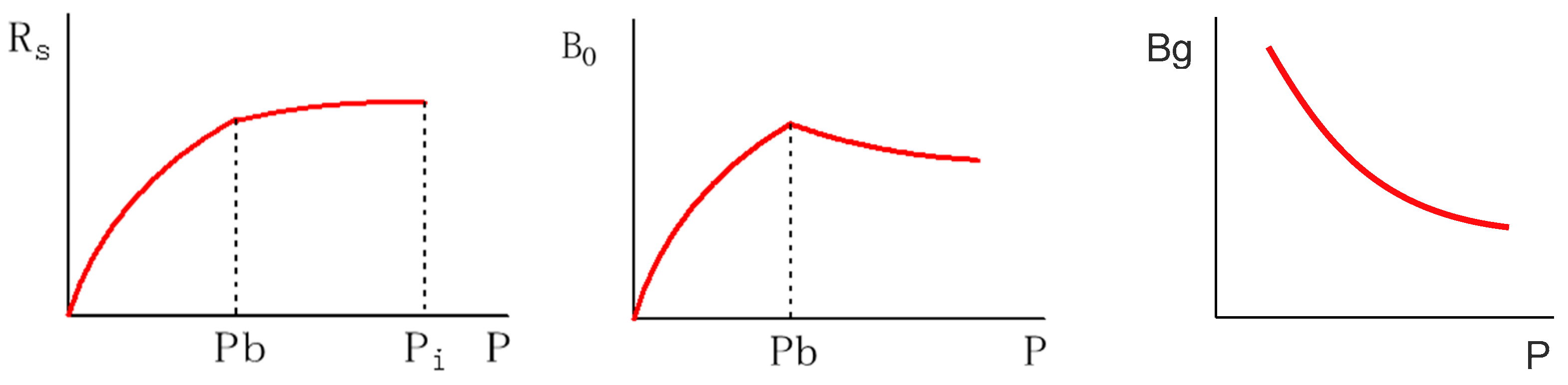
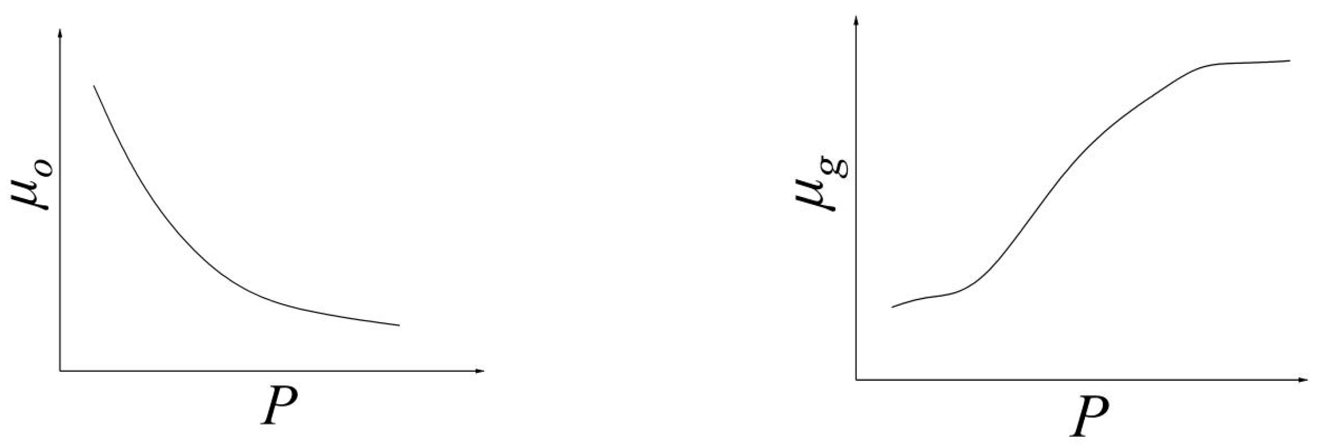
2.1. Simplified Model Calculation of Fluid Physical Properties under Average Pressure Conditions in a Certain Region
- (1)
- At any moment, the porosity, fluid saturation, and relative permeability of the reservoir are uniform.
- (2)
- Regardless of the gas zone and oil zone in the reservoir, the formation pressure is the same, and the volume coefficient, viscosity, and gas dissolution amount of gas and oil are the same.
- (3)
- The influence of gravity is not considered.
- (4)
- At any moment, the oil phase and the gas phase are balanced.
- (5)
- No water intrusion, other than the water output, occurs.
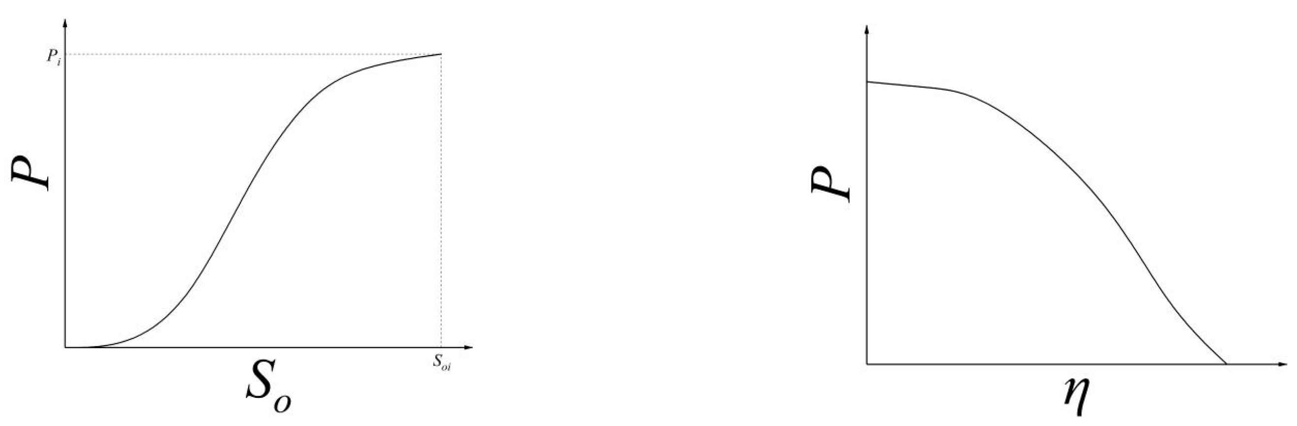
2.2. Simplified Model Calculation of Average Pressure in a Certain Region
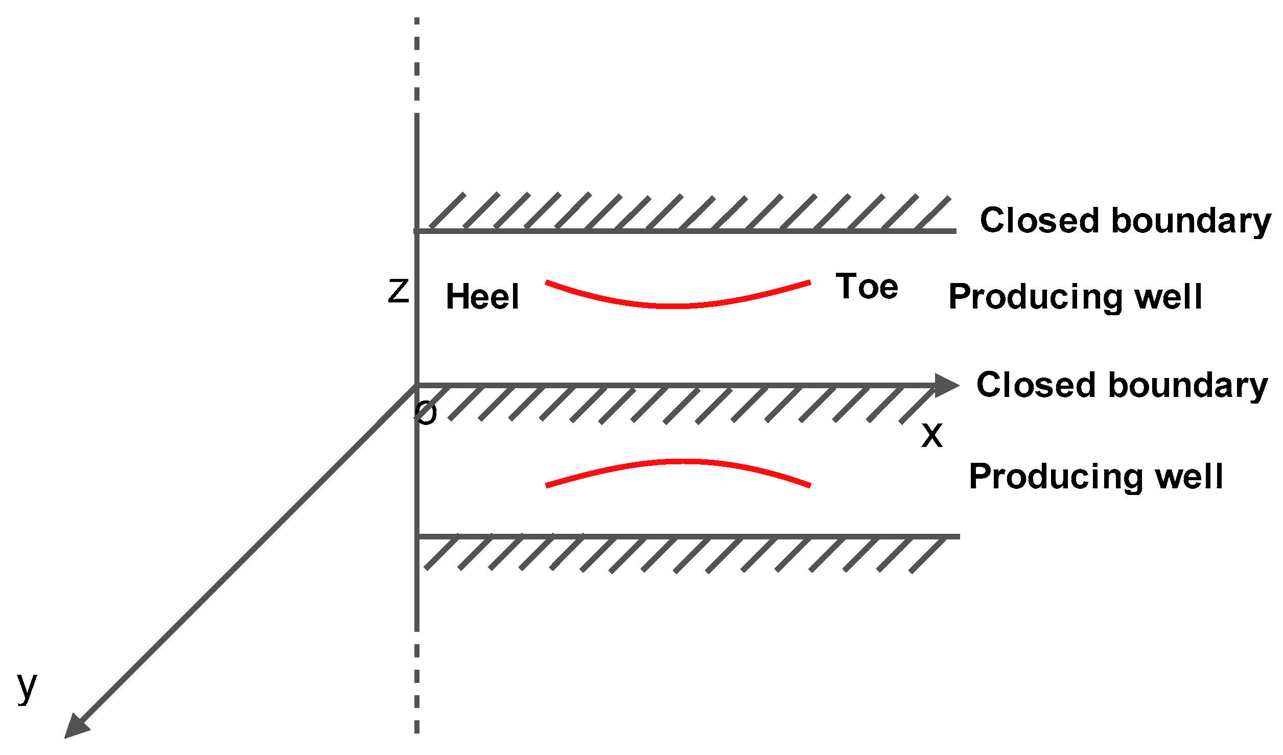
2.3. Calculation of the Three-Dimensional H (Potential) of a Horizontal Well under the Condition of Oil and Gas Two-Phase Flow
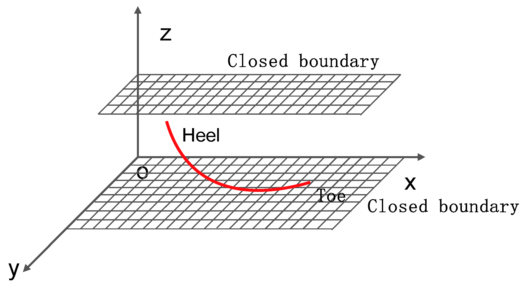
2.4. Calculation of the Potential of Uniform Inflow into a Horizontal Section in a Closed Reservoir
2.5. Horizontal Well Flow
2.6. Coupling Model of the Inflow Performance and Flow in a Wellbore and Its Solution
- (1)
- The circular drainage area is controlled by each well.
- (2)
- The parameters of Kx, Ky, Kz, thickness H, and porosity ϕ are constant throughout the reservoir.
3. Example of the Transient Productivity Prediction Calculation of Oil and Gas Two-Phase Seepage in Horizontal Wells
3.1. Sample Calculation
- (1)
- The basic parameters are shown in Table 1.
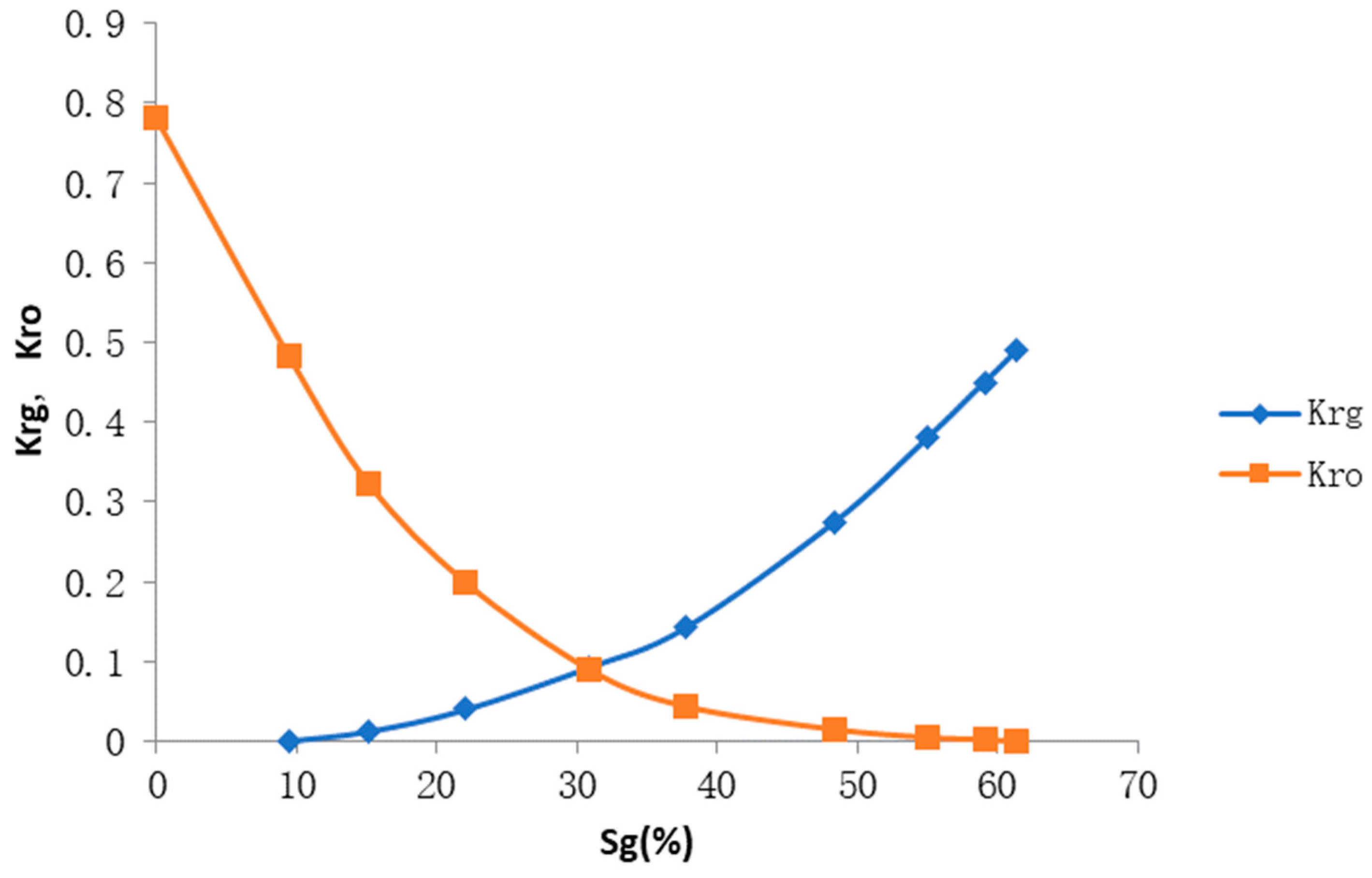
- (2)
- The phase penetration data are shown in Figure 6.
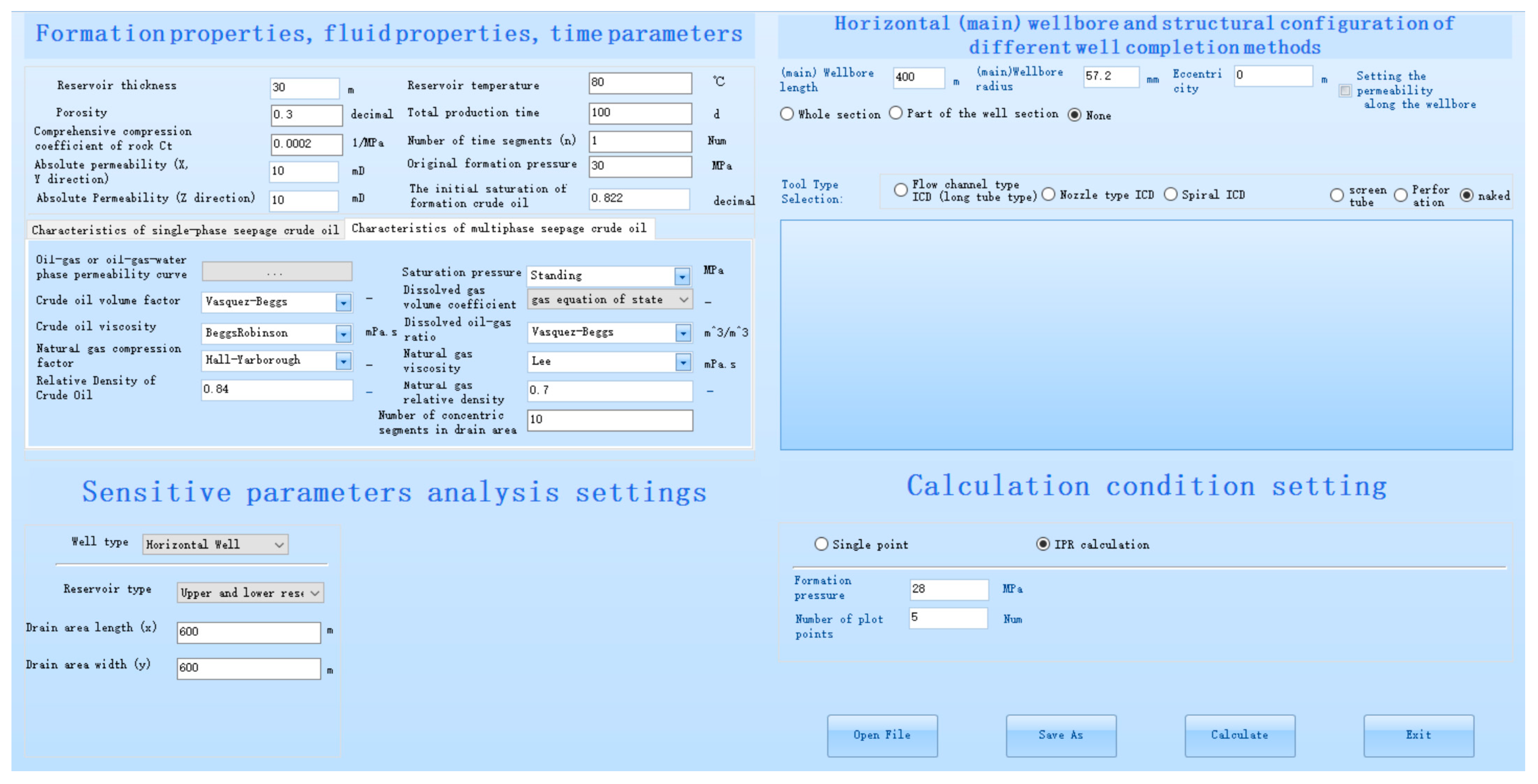
- (3)
- The software interface is shown in Figure 7. The required input parameters and the physical property calculation methods used are shown.
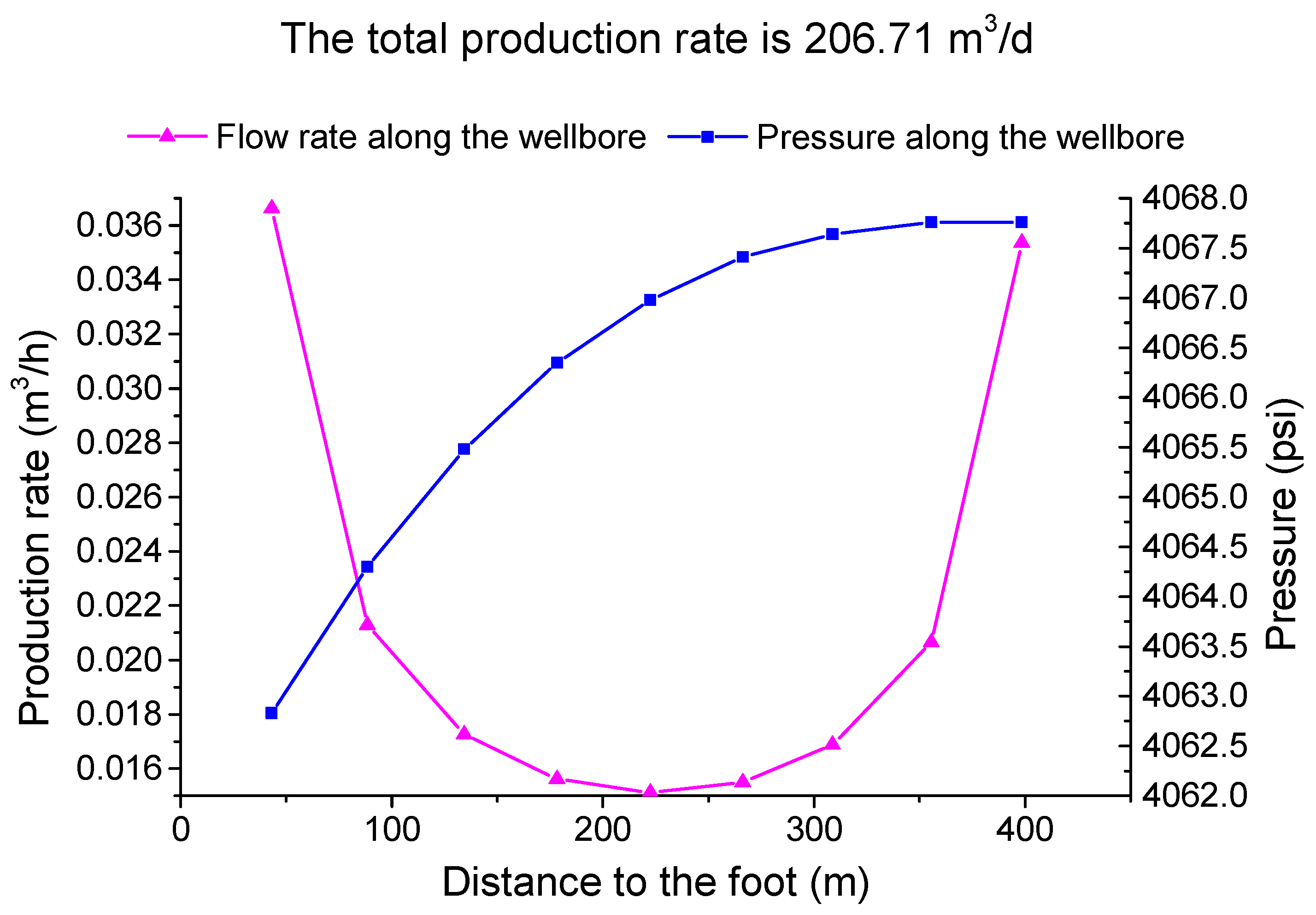
- (4)
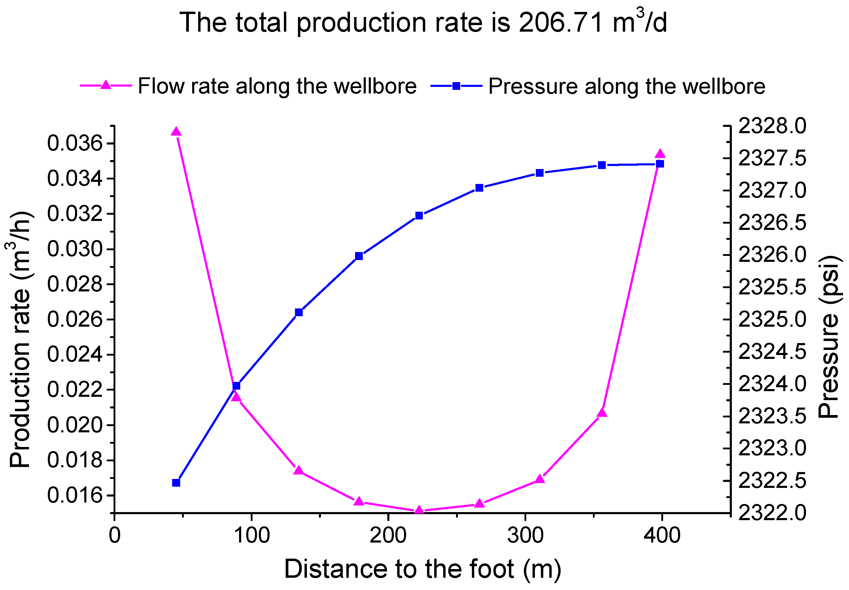
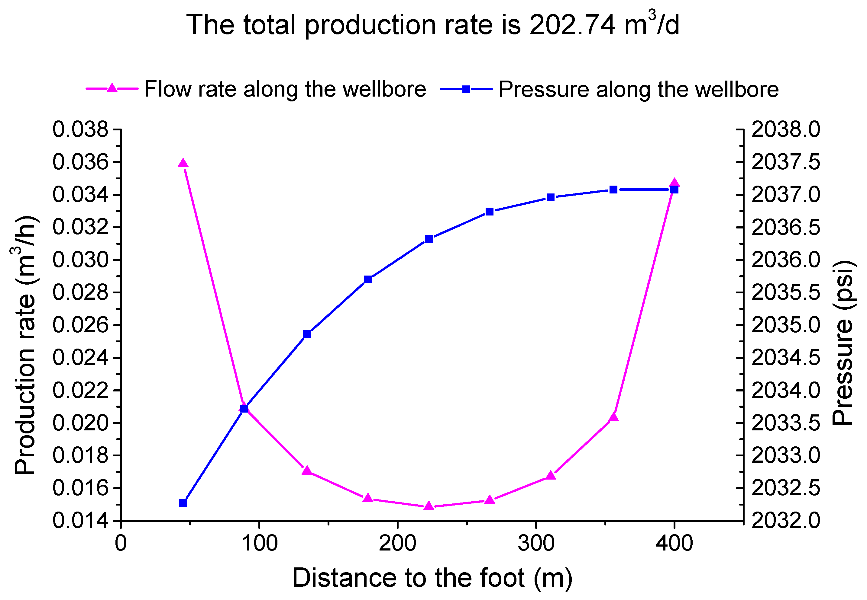
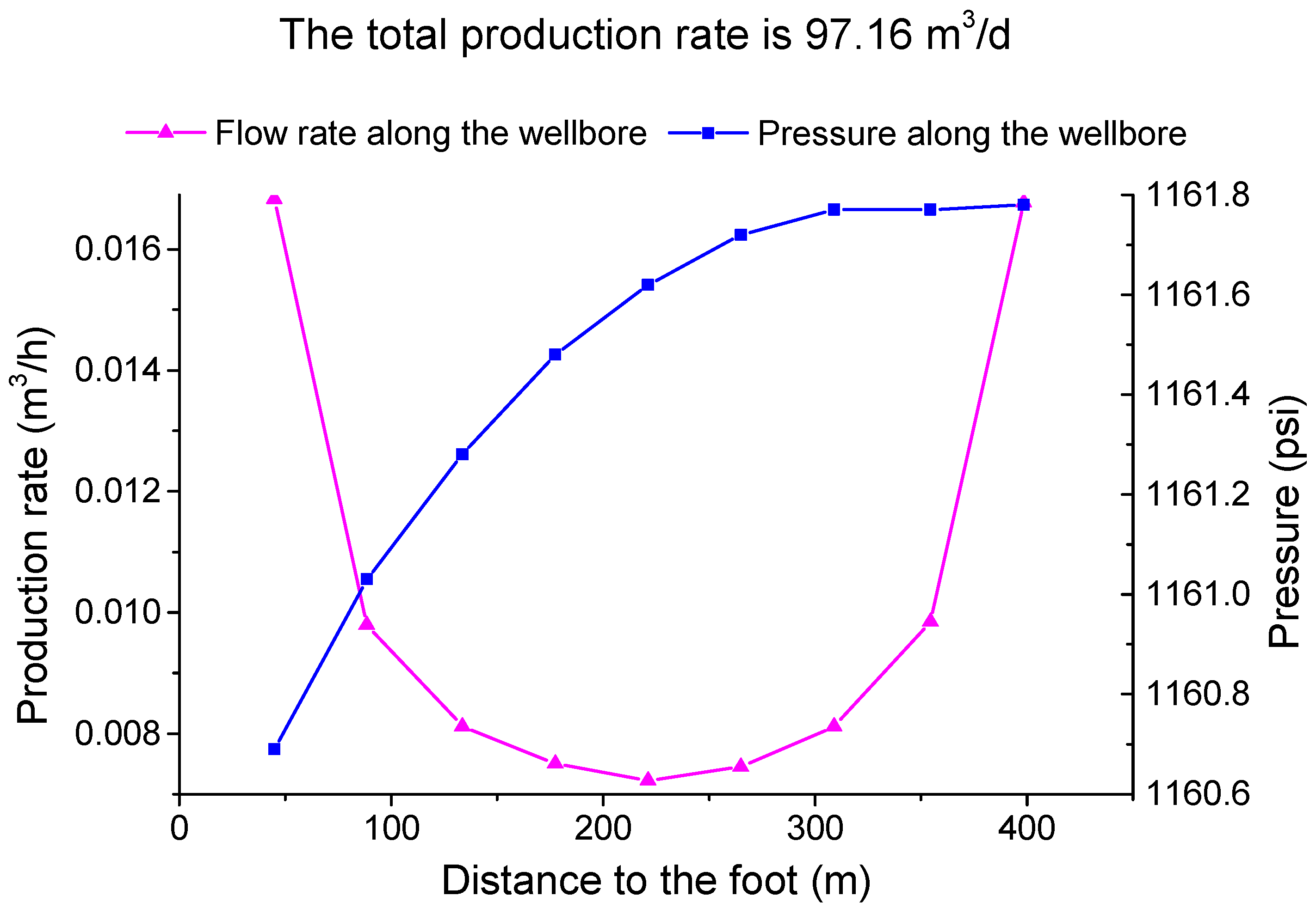
- The result is shown below.
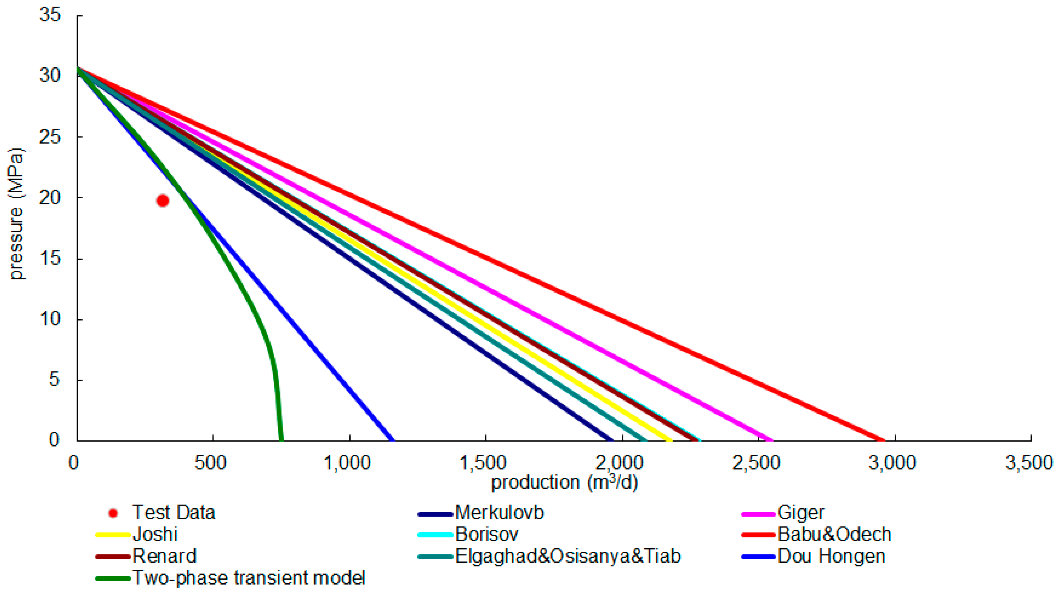
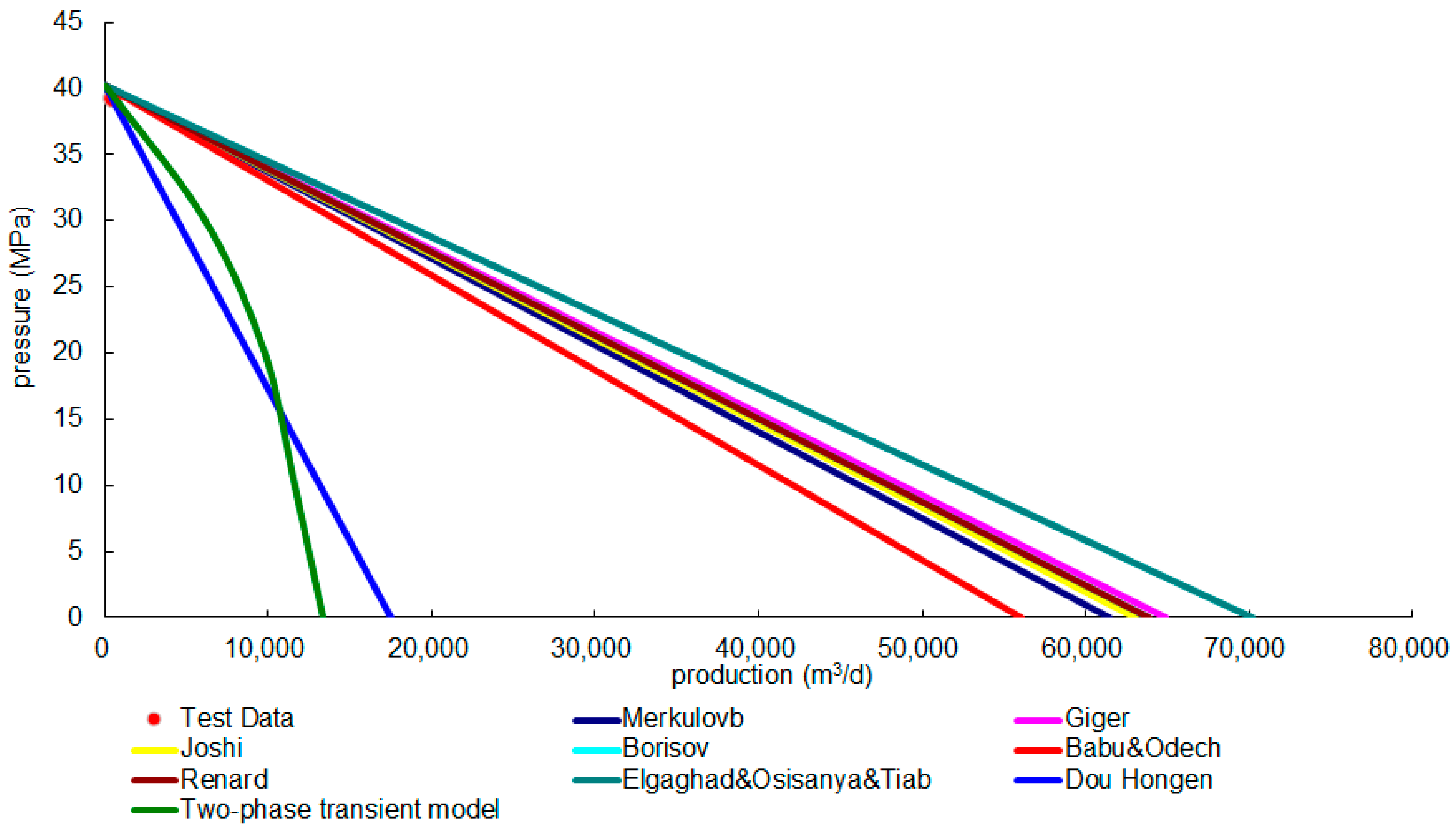
3.2. Verification of the Productivity Prediction of Two Oilfields
- (1)
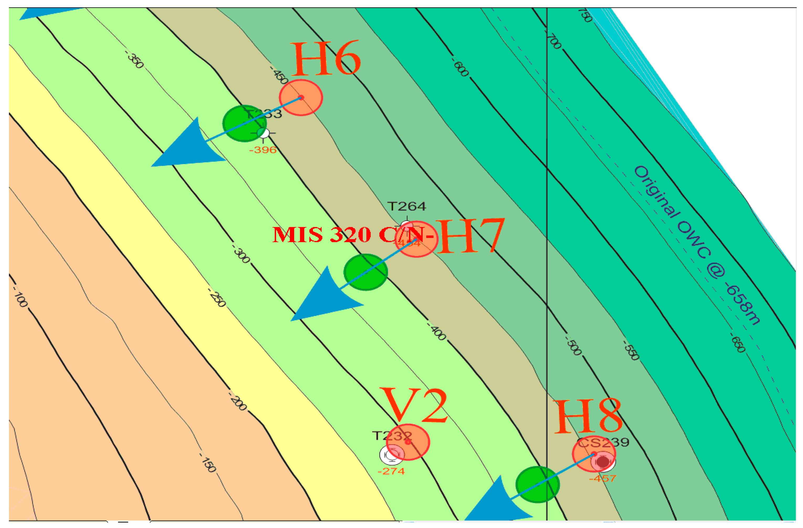
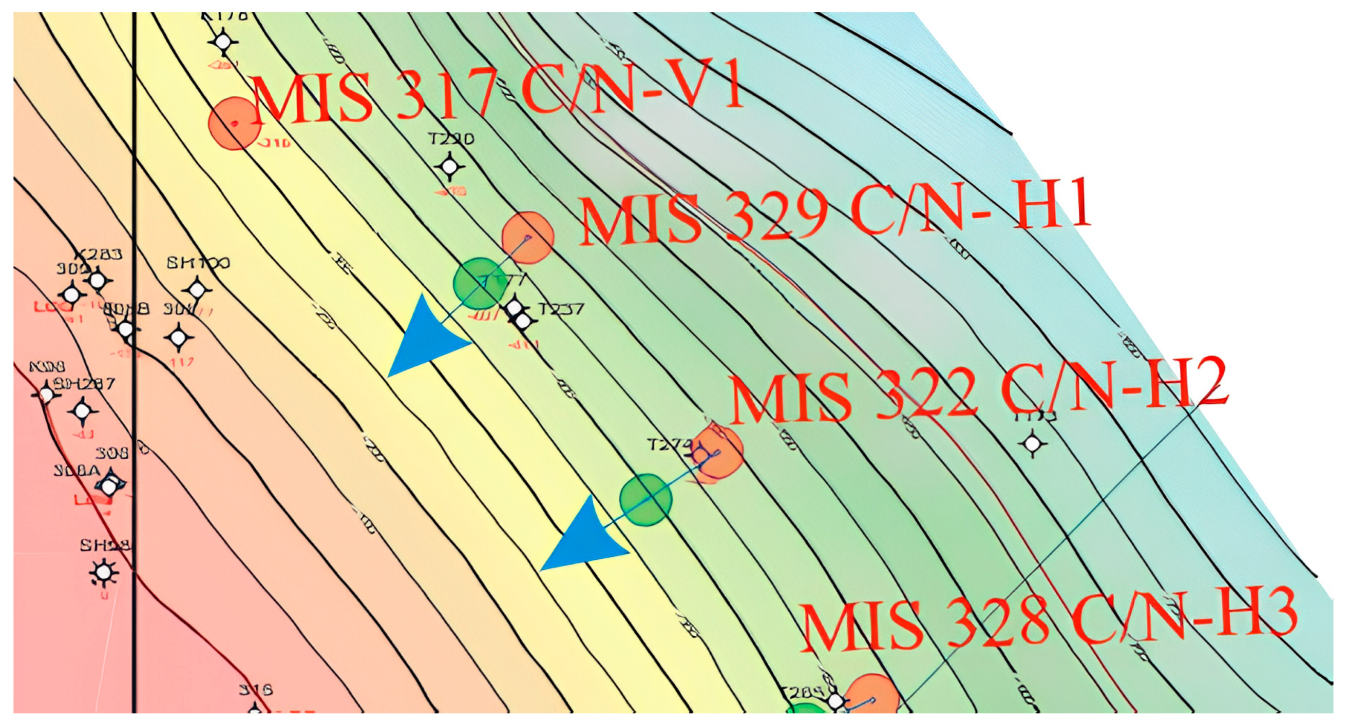
- MIS oilfield, Iran
- (2)
- Hafaya oilfield
4. Conclusions
- (1)
- If the pressure in the reservoir is lower than the saturation pressure, it is difficult to predict the two-phase transient seepage capacity of horizontal wells. Moreover, the reservoir phase permeability changes with pressure, and the variation in the crude oil volume coefficient also changes with pressure. These parameters are a function of pressure. They potentially make the calculation of the horizontal well extremely complicated, and the parameters that vary with pressure need to be considered together. Nevertheless, the relationship between the horizontal well potential (pressure) and production can still be established by using the superposition principle. Then, a capacity prediction model that couples two-phase seepage and wellbore pipe flow in the formation is established. The solution method of the model is given.
- (2)
- The simulation calculation of the established model shows that when the pressure is higher than the saturation pressure, the producing pressure drops, and the oil production rate are the same. When the bottom hole flowing pressure of the well is just lower than the saturation pressure, oil and gas two-phase seepage occurs in the near-well area, while the surrounding area (with a pressure higher than the saturation pressure) undergoes single-phase seepage, and the production decreases. When the formation pressure and bottom hole flowing pressure further decrease, the oil and gas two-phase seepage area in the reservoir will expand, and production will be greatly reduced. Therefore, production should be maintained as high as possible under high formation pressure conditions.
- (3)
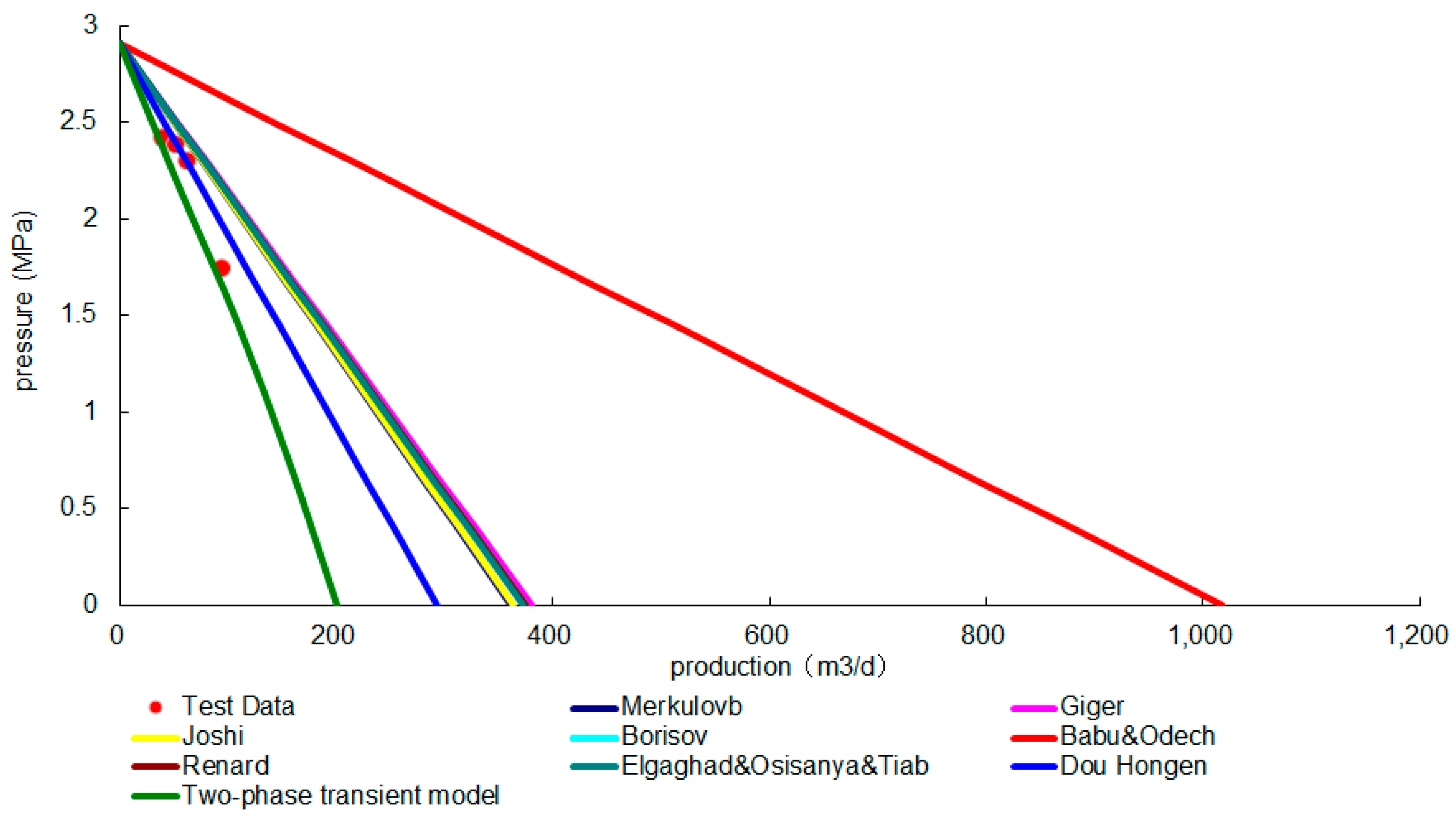
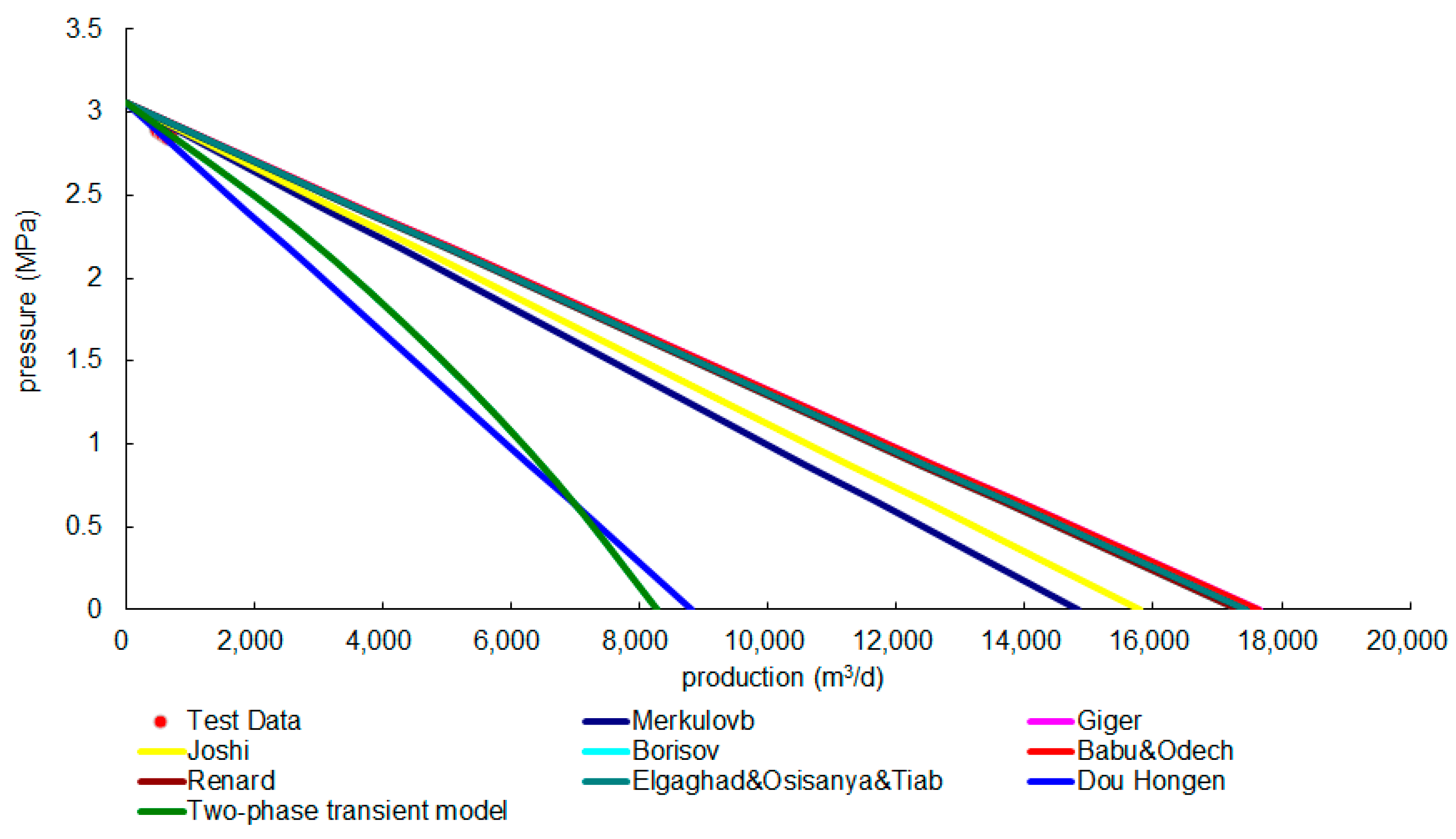
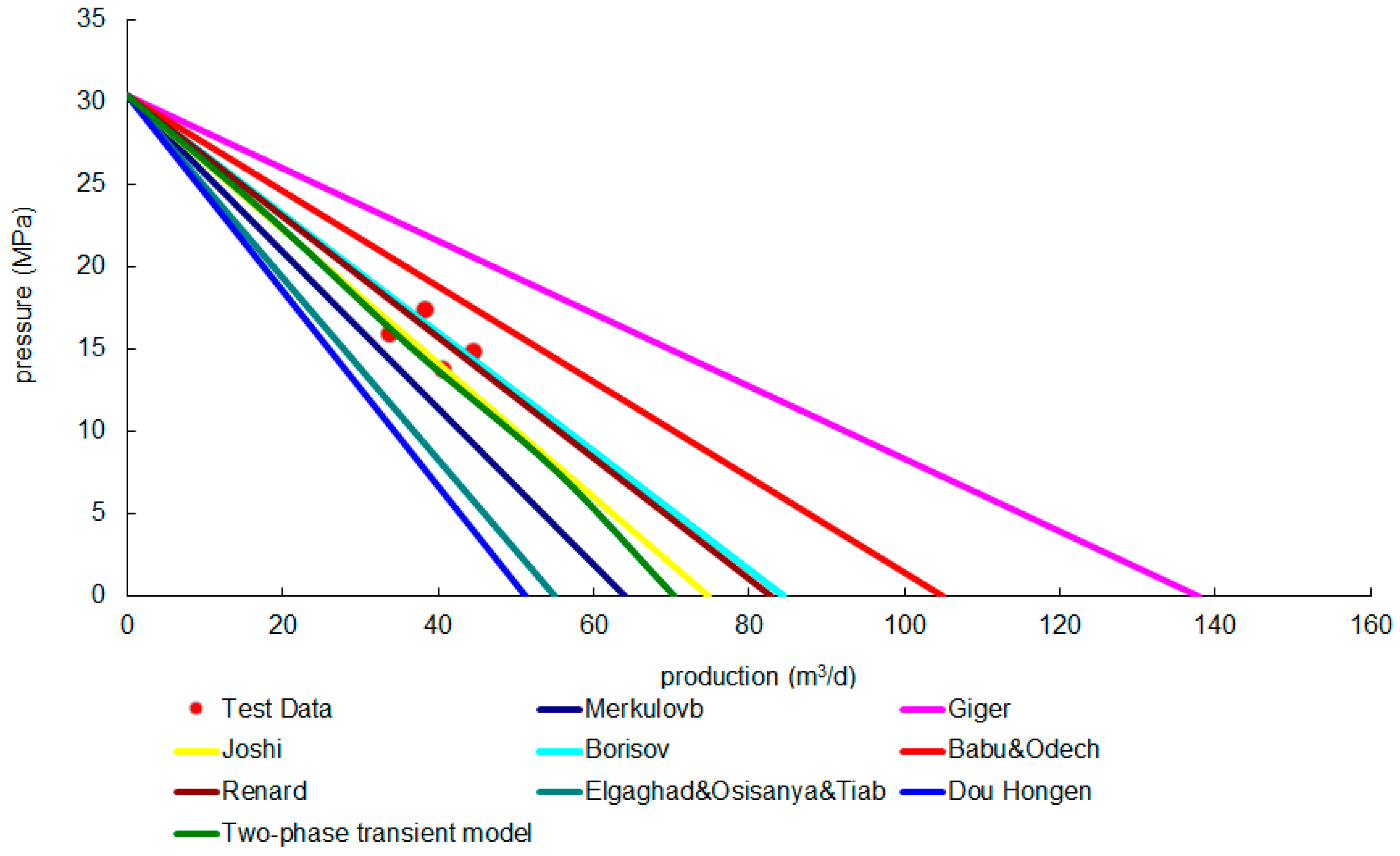
- Through the verification of the productivity prediction of the five wells in two oilfields, the error of the new model is small, and the prediction result is more reliable, which shows that the new model is feasible. Therefore, the new model can predict the oil and gas two-phase productivity of horizontal wells with a simplified reservoir model, no very complex meshing, and only one simulated well. Therefore, the calculation speed will be faster than that of other reservoir numerical simulation methods under the same conditions.
Author Contributions
Funding
Data Availability Statement
Acknowledgments
Conflicts of Interest
References
- Karcher, B.J.; Giger, F.M.; Combe, J. Some Practical Formulas to Predict Horizontal Well Behavior. In Proceedings of the 61st Annual Technical Conference and Exhibition, New Orleans, LA, USA, 5–8 October 1986; SPE Paper 15430. OnePetro: Richardson, TX, USA, 1986. [Google Scholar]
- Lifeng, W.; Chunjiang, C.; Helin, W.; Zeng, N. A review of the development of horizontal well productivity calculation. China Pet. Chem. Ind. 2007, 18, 39–41. [Google Scholar]
- Shedid, A.E.; Samuel, O.O.; Djebbar, T.A. Simple Productivity Equation for Horizontal Wells Based on Drainage Area Concept. In Proceedings of the Western Regional Meeting, Anchorage, AK, USA, 22–24 May 1996; SPE Paper 35713. OnePetro: Richardson, TX, USA, 1996. [Google Scholar]
- Giger, F.M.; Reiss, L.H.; Jourdan, A.P. The Reservoir Engineering Aspects of Horizontal Drilling. In Proceedings of the 59th Annual Technical Conference and Exhibition, Houston, TX, USA, 16–19 September 1984; SPE Paper 13024. OnePetro: Richardson, TX, USA, 1984. [Google Scholar]
- Giger, F.M. Horizontal Wells Production Techniques in Heterogeneous Reservoirs. In Proceedings of the SPE 1985 Middle East Oil Technical Conference and Exhibition, Sakhir, Bahrain, 11–14 March 1985; SPE Paper 13710. OnePetro: Richardson, TX, USA, 1985. [Google Scholar]
- Giger, F.M. Low-Permeability Reservoirs Development Using Horizontal Wells. In Proceedings of the SPE/DOE Low Permeability Reservoirs Symposium, Denver, CO, USA, 18–19 May 1987; SPE Paper 16406. OnePetro: Richardson, TX, USA, 1987. [Google Scholar]
- Joshi, S.D. Augmentation of Well Productivity Using Slant and Horizontal Wells. In Proceedings of the 61st Annual Technical Conference and Exhibition of the Society of Petroleum Engineers, New Orleans, LA, USA, 5–8 October 1986; SPE Paper 15375. OnePetro: Richardson, TX, USA, 1986. [Google Scholar]
- Joshi, S.D. A Review of Horizontal Well and Drainhole Technology. In Proceedings of the 62nd Annual Technical Conference and Exhibition of the Society of Petroleum Engineers, Dallas, TX, USA, 27–30 September 1987; SPE Paper 16868. OnePetro: Richardson, TX, USA, 1987. [Google Scholar]
- Joshi, S.D. Production Forecasting Methods for Horizontal Wells. In Proceedings of the SPE International Meeting on Petroleum Engineering, Tianjin, China, 1–4 November 1988; SPE Paper 17580. OnePetro: Richardson, TX, USA, 1988. [Google Scholar]
- Babu, D.K.; Odeh, A.S. Productivity of a Horizontal Well. SPE Reserv. Eng. 1989, 4, 417–421. [Google Scholar] [CrossRef]
- Renard, G.; Dupuy, J.M. Formation Damage Effects on Horizontal-Well Flow Efficiency. In Proceedings of the 1990 SPE Formation Damage Control Symposium, Lafayette, IN, USA, 22–23 February 1991; SPE Paper 19414. OnePetro: Richardson, TX, USA, 1991. [Google Scholar]
- Dou, H. A New Method of Predicting the Productivity of Horizontal Well. Oil Drill. Prod. Technol. 1996, 18, 76–81. [Google Scholar]
- Chen, Y.-Q. Derivation and Correlation of Production Rate Formula for Horizontal Well. Xinjiang Pet. Geol. 2008, 29, 68–71. [Google Scholar]
- Chen, Y.-Q.; Guo, E.-P. Query, Derivation and Comparison About Joshi’s Production Rate Formula for Horizontal Well in Anisotropic Reservoir. Xinjiang Pet. Geol. 2008, 29, 331–334. [Google Scholar]
- Liu, W.; Tong, D.; Zhang, S. A new method for calculating productivity of horizontal well in low-permeability heavy oil reservoir. Acta Pet. Sin. 2010, 31, 458–462. [Google Scholar]
- Soleimani, M. Naturally fractured hydrocarbon reservoir simulation by elastic fracture modeling. Pet. Sci. 2017, 14, 286–301. [Google Scholar] [CrossRef]
- Soleimani, M. Well performance optimization for gas lift operation in a heterogeneous reservoir by fine zonation and different well type integration. J. Nat. Gas Sci. Eng. 2017, 40, 277–287. [Google Scholar] [CrossRef]
- Jia, X.; Sun, Z.; Lei, G. A new comprehensive formula for productivity prediction of horizontal well. Oil Drill. Prod. Technol. 2019, 41, 78–82. [Google Scholar]
- Li, Y.; Luo, A.; Wu, L.; Yi, X. Shale Productivity Model Considering Stress Sensitivity and Hydraulic Fracture Azimuth. J. Southwest Pet. Univ. Sci. Technol. Ed. 2019, 41, 117–123. [Google Scholar]
- Gao, Y.; Zhang, Y.; Yang, B.; Li, K.; Yuan, Z.; Kang, B.; Zhang, X.; Zhang, X.; Chen, G. Productivity prediction and optimization method of segment length for cross-fault horizontal well in complex fault-block oilfield: A case study of the deepwater oilfield in West Africa. Acta Pet. Sin. 2021, 42, 948–961. [Google Scholar]
- Ma, S.; Li, J.; He, Y.; Liu, C.; Lei, Q.; Huang, T. Multi-Stage Fracturing Seepage Model and Productivity Prediction Method for Horizontal Wells in Shale Oil Reservoir-Use Horizontal Wells in Qingcheng Oil Field, China, as an Example. In Proceedings of the International Petroleum Technology Conference, Bangkok, Thailand, 1–3 March 2023; SPE Paper 22998. OnePetro: Richardson, TX, USA, 2023. [Google Scholar]
- Zhang, Y.; Yang, D. Modeling Two-Phase Flow Behaviour in a Shale Gas Reservoir with Complex Fracture Networks and Flow Dynamics. In Proceedings of the SPE Western Regional Meeting, Anchorage, AK, USA, 22–25 May 2023; SPE Paper 213001. OnePetro: Richardson, TX, USA, 2023. [Google Scholar]
- Liu, P.; Wang, Q.; Luo, Y.; He, Z.; Luo, W. Study on a New Transient Productivity Model of Horizontal Well Coupled with Seepage and Wellbore Flow. Processes 2021, 9, 2257. [Google Scholar] [CrossRef]
- Liu, X.; Guo, C.; Jiang, Z.; Liu, X.; Guo, S. The model coupling fluid flow in the reservoir with flow in the horizontal wellbore. Acta Pet. Sin. 1999, 20, 82–86. [Google Scholar]


| Name | Value | Unit |
|---|---|---|
| Horizontal permeability | 10 | mD |
| Vertical permeability | 10 | mD |
| Crude oil volume factor | 1.281 | |
| porosity | 0.3 | |
| Total compressibility coefficient of formation | 0.0002 | 1/MPa |
| Crude oil viscosity | 0.6365 | mPa.s |
| Reservoir thickness | 30 | m |
| Horizontal well length | 400 | m |
| Original formation pressure | 30 | MPa |
| Bottom hole flowing pressure | 28 | MPa |
| Completion method | Open hole completion | |
| Oil reservoir type | Reservoir with closed upper and lower boundaries | |
| Saturation pressure | 15 | MPa |
| Reservoir temperature | 80 | ℃ |
| Production time | 1 | year |
| Well No. | Oil Layer Thickness m | Porosity Decimal | Comprehensive Compression Factor 1/MPa | Absolute Permeability (in the X and Y Directions) mD | Absolute Permeability (in the Z Direction) mD |
|---|---|---|---|---|---|
| MIS 320 CN-H7 | 157.79 | 0.116 | 0.001276264 | 43 | 43 |
| MIS 322 C/N-H2 | 157.79 | 0.116 | 0.001276264 | 578 | 578 |
| Well No. | Crude Oil Volume Factor | Crude Oil Viscosity | Relative Density of Crude Oil |
|---|---|---|---|
| MIS 320 CN-H7 | 1.09 | 1.8 | 0.832 |
| MIS 322 C/N-H2 | 1.09 | 1.8 | 0.832 |
| Well No. | Well Type | Reservoir Type | Oil Drainage Area Length (x) M | Oil Drainage Area Length (y) m | Wellbore Length m | Wellbore Diameter in | Skin Coefficient in Well Completion | Well Reservoir Factor (m3/MPa) | Formation Pressure MPa |
|---|---|---|---|---|---|---|---|---|---|
| MIS 320 CN-H7 | Horizontal wells | Infinitely large homogeneous reservoirs | 394.1 | 6 1/8” | 10 | 7.093 | 2.91 | ||
| MIS 322 C/N-H2 | 157.79 | Infinitely large homogeneous reservoirs | 1524 | 1524 | 422.34 | 6 1/8” | −3 | 7.093 | 3.059 |
| No. | Duration | ESP (Hz) | Pwf (psi) | Δp (psi) | Rate (bbl/d) | PI (bbl/d/psi) |
|---|---|---|---|---|---|---|
| 1 | 22:00–2:00 | 35 | 351 | 72 | 255 | 3.86 |
| 2 | 2:04–6:15 | 40 | 346 | 77 | 330 | |
| 3 | 6:19–10:15 | 45 | 333 | 90 | 398 | |
| 4 | 10:21–16:00 | 50 | 252 | 171 | 596 |
| No. | Oil Rate (bbl/d) | ΔP (psi) | Pwf (psi) | Watercut (%) | Choke Size (1/64”) | ESP (Hz) | PI (bbl/d/psi) |
|---|---|---|---|---|---|---|---|
| 1 | 3392 | 25 | 419 | 0.2 | 42 | 45 | 136.57 |
| 2 | 3820 | 28 | 416 | 0.2 | 52 | 47 | |
| 3 | 4260 | 31 | 413 | 0.1 | 50 | 50 |
| Method | Merkulovb | Giger | Joshi | Borisov | Babu & Odech | Renard | Elgaghad | Dou Hongen | Multiphase Flow Transient Model |
|---|---|---|---|---|---|---|---|---|---|
| Absolute average relative error (decimal) | 0.369 | 0.442 | 0.378 | 0.422 | 2.859 | 0.422 | 0.413 | 0.120 | 0.096 |
| Method | Merkulovb | Giger | Joshi | Borisov | Babu & Odech | Renard | Elgaghad | Dou Hongen | Multiphase Flow Transient Model |
|---|---|---|---|---|---|---|---|---|---|
| Absolute average relative error (decimal) | 0.519 | 0.808 | 0.617 | 0.775 | 0.806 | 0.775 | 0.787 | 0.097 | 0.103 |
| Well No. | Oil layer Thickness m | Porosity Decimal | Comprehensive Compression Factor 1/MPa | Absolute Permeability (in the X and Y Directions) mD | Absolute Permeability (in the Z Direction) mD | Oil Layer Temperature ℃ |
|---|---|---|---|---|---|---|
| HF003-S001H | 70 | 0.177 | 0.0013154 | 0.076 | 0.02736 | 81.2 |
| HF002-M001H | 30 | 0.115 | 0.001285 | 13.4 | 93.78 | |
| HF001-N002H | 8 | 0.197 | 0.00174 | 861 | 114.27 |
| Well No. | Crude Oil Volume Factor | Crude Oil Viscosity | Relative Density of Crude Oil |
|---|---|---|---|
| HF003-S001H | 1.237 | 1.33 | 0.904 |
| HF002-M001H | 1.55 | 1.643 | 0.794 |
| HF001-N002H | 1.444 | 0.64 | 0.872 |
| Well no. | Well Type | Reservoir Type | Wellbore Length m | Wellbore Diameter in | Skin Coefficient in Well Completion | Well Reservoir Factor (m3/MPa) | Formation Pressure MPa |
|---|---|---|---|---|---|---|---|
| HF003-S001H | Horizontal wells | Boundary homogeneous reservoirs | 532.1 | 0.15 | −5.69 | 2.49 | 30.38 |
| HF002-M001H | Horizontal wells | Infinitely large homogeneous reservoirs | 579 | 0.15 | −5.47 | 5.99 | 30.659 |
| HF001-N002H | Horizontal wells | 273 | 0.15 | −3.51 | 40.22 |
| Date | Time | Choke Size (in) | WHP (psi) | Flowing-Pressure (psi) | Differential Pressure (psi) | Production Rate | |
|---|---|---|---|---|---|---|---|
| Oil (bbl/d) | Gas (Mscf/d) | ||||||
| 29.8.2011 | 14:53 | 16/64 “ | / | 2522.46 | 1760.4 | 241.6 | 161.2 |
| 30.8.2011 | 2:23 | 20/64 “ | / | 2141.11 | 2141.75 | 280.6 | 167.1 |
| 30.8.2011 | 10:42 | 24/64 “ | / | 1990.89 | 2291.97 | 255.6 | 221.8 |
| 30.8.2011 | 16:23 | 16/64 “ | / | 2301.37 | 1981.49 | 213.5 | 109.7 |
| Choke Size (in) | WHP (psia) | Flowing Pressure (psia) | Differential Pressure (psi) | Production Rate | ||
|---|---|---|---|---|---|---|
| Fluid (bbl/d) | Oil (bbl/d) | Gas–Oil Ratio (scf/bbl) | ||||
| 48/64 | 450 | 2870.405 | 1454.19 | 1992 | 1992 | 976 |
| Oil Production Rate (bbl/d) | Flowing Pressure (psi) |
|---|---|
| 3263.6 | 5693.99 |
| Method | Merkulovb | Giger | Joshi | Borisov | Babu & Odech | Renard | Elgaghad | Dou Hongen | Multiphase Flow Transient Model |
|---|---|---|---|---|---|---|---|---|---|
| Absolute average relative error (decimal) | 0.196 | 0.731 | 0.092 | 0.104 | 0.318 | 0.102 | 0.309 | 0.356 | 0.098 |
| Method | Merkulovb | Giger | Joshi | Borisov | Babu & Odech | Renard | Elgaghad | Dou Hongen | Multiphase Flow Transient Model |
|---|---|---|---|---|---|---|---|---|---|
| Absolute average relative error (decimal) | 1.195 | 1.849 | 1.436 | 1.552 | 2.308 | 1.542 | 1.332 | 0.297 | 0.257 |
| Method | Merkulovb | Giger | Joshi | Borisov | Babu & Odech | Renard | Elgaghad | Dou Hongen | Multiphase Flow Transient Model |
|---|---|---|---|---|---|---|---|---|---|
| Absolute average relative error (decimal) | 1.829 | 1.987 | 1.901 | 1.940 | 1.580 | 1.940 | 2.230 | 0.194 | 0.116 |
| Forecasting Methodology | Merkulovb | Giger | Joshi | Borisov | Babu & Odech | Renard | Elgaghad | Dou Hongen | Multiphase Flow Transient Model |
|---|---|---|---|---|---|---|---|---|---|
| MIS 320 CN-H7 | 0.369 | 0.442 | 0.378 | 0.422 | 2.859 | 0.422 | 0.413 | 0.12 | 0.096 |
| MIS 322 CN-H2 | 0.519 | 0.808 | 0.617 | 0.775 | 0.806 | 0.775 | 0.787 | 0.097 | 0.103 |
| HF003-S001H | 0.196 | 0.731 | 0.092 | 0.104 | 0.318 | 0.102 | 0.309 | 0.356 | 0.098 |
| HF002-M001H | 1.195 | 1.849 | 1.436 | 1.552 | 2.308 | 1.542 | 1.332 | 0.297 | 0.257 |
| HF001-N002H | 1.829 | 1.987 | 1.901 | 1.94 | 1.58 | 1.94 | 2.23 | 0.194 | 0.116 |
| Average error | 0.8216 | 1.1634 | 0.8848 | 0.9586 | 1.5742 | 0.9562 | 1.0142 | 0.2128 | 0.134 |
Disclaimer/Publisher’s Note: The statements, opinions and data contained in all publications are solely those of the individual author(s) and contributor(s) and not of MDPI and/or the editor(s). MDPI and/or the editor(s) disclaim responsibility for any injury to people or property resulting from any ideas, methods, instructions or products referred to in the content. |
© 2023 by the authors. Licensee MDPI, Basel, Switzerland. This article is an open access article distributed under the terms and conditions of the Creative Commons Attribution (CC BY) license (https://creativecommons.org/licenses/by/4.0/).
Share and Cite
Ke, W.; Luo, W.; Miao, S.; Chen, W.; Hou, Y. A Transient Productivity Prediction Model for Horizontal Wells Coupled with Oil and Gas Two-Phase Seepage and Wellbore Flow. Processes 2023, 11, 2012. https://doi.org/10.3390/pr11072012
Ke W, Luo W, Miao S, Chen W, Hou Y. A Transient Productivity Prediction Model for Horizontal Wells Coupled with Oil and Gas Two-Phase Seepage and Wellbore Flow. Processes. 2023; 11(7):2012. https://doi.org/10.3390/pr11072012
Chicago/Turabian StyleKe, Wenqi, Wei Luo, Shiyu Miao, Wen Chen, and Yaodong Hou. 2023. "A Transient Productivity Prediction Model for Horizontal Wells Coupled with Oil and Gas Two-Phase Seepage and Wellbore Flow" Processes 11, no. 7: 2012. https://doi.org/10.3390/pr11072012
APA StyleKe, W., Luo, W., Miao, S., Chen, W., & Hou, Y. (2023). A Transient Productivity Prediction Model for Horizontal Wells Coupled with Oil and Gas Two-Phase Seepage and Wellbore Flow. Processes, 11(7), 2012. https://doi.org/10.3390/pr11072012