Article

Research on a Photovoltaic Power Prediction Model Based on an IAO-LSTM Optimization Algorithm

College of Electronic and Information, Taiyuan University of Science & Technology, Taiyuan 030024, China
*
Author to whom correspondence should be addressed.
Processes 2023, 11(7), 1957; https://doi.org/10.3390/pr11071957
Submission received: 4 June 2023 / Revised: 21 June 2023 / Accepted: 24 June 2023 / Published: 28 June 2023
(This article belongs to the Special Issue Process Design and Modeling of Low-Carbon Energy Systems)

Abstract

:
With the rapid popularization and development of renewable energy, solar photovoltaic power generation systems have become an important energy choice. Convolutional neural network (CNN) models have been widely used in photovoltaic power forecasting, with research focused on problems such as long training times, forecasting accuracy and insufficient speed, etc. Using the advantages of swarm intelligence algorithms such as global optimization, strong adaptability and fast convergence, the improved Aquila optimization algorithm (AO) is used to optimize the structure of neural networks, and the optimal solution is chosen as the structure of neural networks used for subsequent prediction. However, its performance in processing sequence data with time characteristics is not good, so this paper introduces a Long Short-Term Memory (LSTM) neural network which has obvious advantages in time-series analysis. The Cauchy variational strategy is used to improve the model, and then the improved Aquila optimization algorithm (IAO) is used to optimize the parameters of the LSTM neural network to establish a model for predicting the actual photovoltaic power. The experimental results show that the proposed IAO-LSTM photovoltaic power prediction model has less error, and its overall quality and performance are significantly improved compared with the previously proposed AO-CNN model.

1. Introduction

With global energy demand increasing and the problem of climate change worsening, photovoltaic power generation as an environmentally friendly, renewable and reliable new energy source, is increasingly applied on a global scale. It is well known that photovoltaic power generation systems are greatly affected by environmental conditions, such as light intensity, temperature, wind speed, and so on. They also have impacts and challenges for the power system and bring greater security risks. Therefore, how to accurately predict the power generation of photovoltaic power generation systems is the key to ensuring their stable operation. At the same time, it can also help power system operators make real-time dispatch decisions, reduce the security risk of power grids, improve the quality of power supply and provide economic benefits [1,2,3].
By predicting the output power of photovoltaic power generation, the optimal dispatching of power grids can be realized, the stability level of power systems can be effectively improved, and the potential safety problems in power systems can be eliminated. It can also effectively reduce the output limit of photovoltaic power generation systems and increase the rate of return on investment, thus increasing the economic benefits and operation management level of photovoltaic power generation systems. At present, the commonly used methods for PV power prediction include physical methods [3], statistical methods [4,5,6], meta-heuristic learning methods [7,8] and combination methods [9], etc.
Swarm intelligence algorithms are a kind of intelligent optimization method that solve practical problems by simulating the swarm intelligence behaviors of natural organisms. Neural networks are a network structure composed of many neurons, which can learn complex nonlinear relationships adaptively, and have good performance in prediction and classification. In recent years, more and more scholars combine swarm intelligence algorithms with neural networks for PV power prediction. For example, Wang et al. proposed a deterministic and probabilistic prediction of photovoltaic power based on deep convolutional neural networks, which can improve prediction accuracy [10]. In [11], an artificial neural network is used to reduce the complexity of a PV power prediction model and improve its prediction accuracy. The advantage of a hybrid method is that it can make full use of the advantages of both methods and improve prediction accuracy and efficiency.
Various artificial intelligence technologies with adaptive and self-learning abilities have been developed and are gradually becoming more widely used in the field of electric power. Through a comparative study of various methods, this paper adopts the method combining LSTM and optimization methods to realize photovoltaic output power prediction. Compared with regular CNN networks, an LSTM network is more suitable for processing classification or prediction of time-series data. By introducing a gate structure, an LSTM neural network has greater selectivity compared with traditional recursive neural networks [12,13,14,15,16,17,18,19,20,21,22,23]. In this paper, a neural network model based on the Aquila optimization algorithm combined with a neural network prediction model is proposed to speed up the prediction speed of the neural network and improve the prediction accuracy and speed of photovoltaic power systems. Then, the Aquila optimization algorithm (IAO) is used to optimize the parameters of the LSTM neural network to establish a model for predicting the actual photovoltaic power. The proposed IAO-LSTM photovoltaic power prediction model reduces error and its overall quality and performance are significantly improved compared with AO-CNN models.

2. Photovoltaic Power Data Preprocessing

Domestic and foreign research studies generally choose irradiance, temperature, wind direction and wind speed as the main influencing factors of photovoltaic power generation. In different distributed photovoltaic power stations, considering that the direct installation angle and position of the photovoltaic array are not exactly the same, different effects will gradually form. However, according to the connection between meteorological factors and the rated output power of photovoltaic new energy, determining more reasonable meteorological factors will help to further improve the accuracy of power prediction. For specific analysis of relevant data, the internal relationship between different functions can be used to judge the correlation between different functions through a curve, so as to understand the degree of correlation of independent variables and dependent variables according to the data. The correlation coefficient refers to the correlation between the variable and parameters of the function. If the value is regular, it is considered as positive correlation, and if the value is less than zero, it is considered a negative correlation. From the correlation analysis, it can be found that for photovoltaic arrays, it is reasonable to select the influence of irradiance, temperature, wind speed and wind direction.
The problem of missing or abnormal data caused by abnormal local function is inevitable, and photovoltaic power generation and various meteorological factors, such as light intensity, ambient temperature, wind speed and other unit function relationships are not the same. Therefore, the original data must be preprocessed to obtain data that can be directly applied in model training and prediction. In the data preprocessing, data outliers are corrected, missing data are completed, and the data are normalized.
(1)
There is a strong correlation between PV power and meteorological data. Missing values are replaced with the mean of values before and after the missing value. If a large amount of data are missing during the day, the data for that day are deleted to prevent human influence. Replacement of missing data can be performed using the following formula:
data j = d a t a j 5 + d a t a j 4 + d a t a j 1 + d a t a j + 1 + d a t a j + 4 d a t a j + 5 10
The data between five moments before and after the missing data are selected to calculate the mean value to supplement the missing data, and Formula (1) shows the value between the left and right five moments of the missing data, respectively, as can be seen from (1).
(2)
If there is no significant change in radiance or other meteorological data but the data on photovoltaic power generation have changed significantly, this value needs to be removed. In addition, if the photoelectric energy is negative, then in the case of very low radiation or zero, 0 is used instead of the negative value.
(3)
The resolution frame rate of the database data is changed. The data interval needed to predict actual PV power over a short period of time is between 15 min and 1 h. Given the short time span of minute-level database data, the application of the original 1 min resolution data is not common and even less in production practice. The data collected are, therefore, converted into 15 min resolution.
(4)
Data normalization is necessary. Because meteorological factors such as solar radiation have different dimensions, directly introducing them into the model reduces the accuracy of power prediction. Normalization of data can speed up model training and improve prediction accuracy. In general, maximum and minimum principles are used in combination for data normalization, and the formula is as follows:
d a t a i = d a t a i d a t a max d a t a min d a t a max
where d a t a i represents the value to be normalized, d a t a min and d a t a max represent the minimum value and the maximum value, respectively.

3. Principle of Convolutional Neural Networks

A convolutional neural network (CNN) is a relatively simple neural network used to solve prediction and classification problems. However, this algorithm requires much data to predict the model and its structural parameters directly affect the accuracy and generalization ability of the model, which also makes it difficult to determine the parameters. In order to obtain better results, the accuracy of CNN prediction models must be further improved.
In a CNN, the neural model refers to the convolutional nucleus (also known as a filter) in the convolutional layer. The filter is a small two-dimensional weight matrix, usually much smaller than the input image. In a CNN, the filter performs convolutional operations on different local regions of the input data to extract local features of the image. Each filter has a set of learnable weight parameters that are gradually adjusted by backpropagation and gradient-descent optimization. In forward propagation, the convolutional core sliding window scans different positions of the input image, convolves each position and generates a new feature map. In this process, each weight of the convolutional nucleus is equivalent to the weight of the neuron, which is used to control the response of the different information in the input data to the convolutional nucleus.
The neural network model is the basic structure of a deep neural network and has wide applicability. The advantage of this method is that it can effectively extract the external resources needed for global reinforcement training and complete the final classification task by using the external features of the local organization of the database data. The CNN architecture comprises a multi-layered feedforward neural network of convolutional layers, pooled layers, and fully connected layers. After a series of convolutional operations on the input data, the neural network extracts information from the simplest features and gradually becomes more complex until it can uniquely define the target’s eigenvalues.
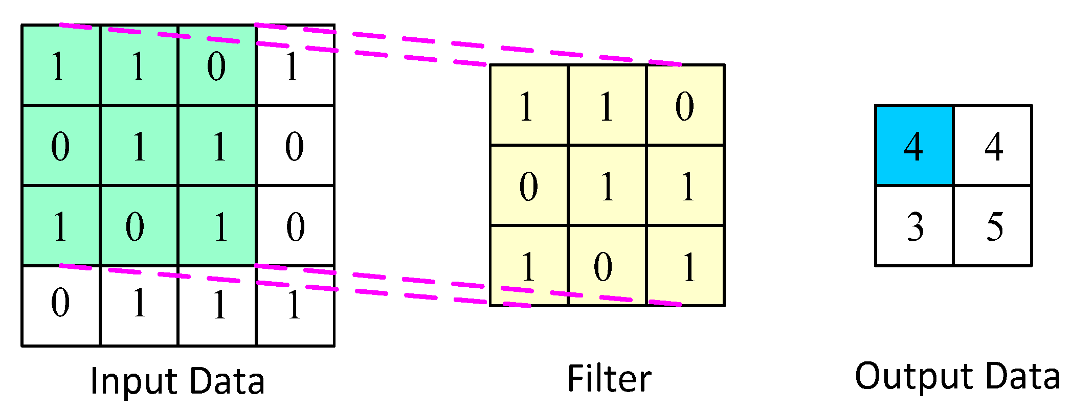
As shown in Figure 1, in the CNN model, the input layer is the point layer, which preprocesses the input display image. Preprocessing standardizes the display image, maintains its balance, rotates and moves it in parallel, converts the image into a mirror file, and converts perspective. Then, the input image data are transformed into a digital vector, and the image range is reduced to a numerical region suitable for the activation function. A hidden layer is a convolutional layer that includes one or more convolutional layers and one or more fully connected layers. The convolutional layer is the CNN core layer that performs most of the calculations. This layer convolves the input data with the filter and passes the result to the next layer. Convolution is a linear operation, similar to traditional neural networks. he operation is ordered, multiplying the input data one by one with the filter, and calculating the sum of the products at each spatial location. The convolution layer contains a set of filters, each convolving the input matrix. In this operation, the filter slides along the vertical and horizontal directions of the input matrix to compute the sum of the products at each spatial position. The green region is the region corresponding to the filter selected from the input data. The yellow area is the filter, and the blue area is the output data corresponding to the selected filter. The convolution process is shown in Figure 2.
In the training process, the weight in the filter is adjusted by back propagation and gradient descent to minimize the model’s loss function. The convolution calculation process is given by the formula below. The mathematical expression of neurons in the convolution layer is as follows:
x m y = f ( n X x n y 1 * k m n y + b m y )
where x m y is the eigen graph matrix corresponding to the n-th feature graph of the (y − 1) layer, k m n y is the weight matrix corresponding to the mn-th feature graph of the y layer, * is the convolution operator, b m y is the deviation value of the m feature graph of the n layer, and f is the activation function. After convolution, the Eigen map matrix x m y is composed of the neurons of the m eigen map of the y layer.
x m y = f 1 ( n X x n y 1 * k m n y + b m y )
There are two common pooling methods in the pooling layer. One is the maximum function pool, the other is the average function pool. Maximum pooling selects the maximum value of an area as the output of the response, and average pooling selects the arithmetic mean of an area as the output response. The mathematical expression for the pool layer is:
x m y = f 1 ( a m y p o o l ( x m y 1 ) + b m y )
where pool is the pooling function, and a and b are the deviation values of each feature graph, respectively. Excitation function convolution is performed on the linear transformation layer. Therefore, when joining several hidden layers, the input and output show linear correlation. As a result, its performance is limited by a certain level of approximation. In practice, convolutional neural networks are not just linear operations.

4. Aquila Optimization Algorithm

The Aquila optimization algorithm is a new intelligent optimization algorithm [20,21,22,23]. It is mainly used to solve real number optimization problems. This algorithm has many exploration and development strategies. Compared with other meta-heuristic algorithms, the Aquila optimization algorithm has obvious advantages. The algorithm was inspired by four swarm behaviors of Northern Aquila birds during predation: (1) expanding the search area by soaring vertically and hunting birds in flight; (2) flying by contours of short gliding attacks and attacking prey in low-level air near the ground; (3) attacking prey gradually by low-flying and slow descent; and (4) walking and catching prey on land by diving. The initialization process is as follows: first, it randomly initializes the population position matrix as follows:
X i j = r a n d × ( U B j L B j ) + L B j , i = 1 , 2 , , D i m
where rand is a random vector, L B j represents the j-th lower bound for a given problem, and U B j represents the j-th upper bound for a given problem.
(1)
Expand the exploration is the first stage when the Aquila is hunting birds in the air. The birds use vertical glide height to expand the search scope. Its mathematical formula is:
X 1 ( t + 1 ) = X b e s t ( t ) × ( 1 t T ) + ( X M ( t ) X b e s t ( t ) × r a n d )
X M ( t ) = 1 N i = 1 N X i ( t ) , j = 1 , 2 , , D i m
where X ( t ) and X ( t + 1 ) represent the individual position of the AO algorithm in the t iteration and the t + 1 iteration, respectively, X b e s t ( t ) represents the optimal individual position obtained by the algorithm at the t iteration, X M ( t ) is the average position of the population in the t iteration, and T is the maximum number of iterations.
(2)
Downsizing is the second stage when the Aquila flock finds its prey from high in the air. It chooses to spiral over the target, prepares to land, and then attacks. The mathematical expression can be shown as:
X 2 ( t + 1 ) = X b e s t ( t ) × Levy ( D ) + X R ( t ) + ( y x ) × r a n d
where Levy (D) is the Levis strategy, s is a constant with the value 0.01, and u and v are random numbers between 0 and 1.
Levy ( D ) = s × u × σ | v | 1 p
σ = [ τ ( 1 + β ) × sin e ( π β 2 ) τ ( 1 + β 2 ) × β × 2 ( β 1 2 ) ]
Here, τ ( x ) is a Gamma function and β is a constant with a fixed value of 1.5. x and y represent the shape of a spiral flight. r is the search step, the radius of the helix. D 1 is the integer matrix from 1 to the length of the search space. θ is the helix angle, and θ 1 is the initial helix angle.
y = r × cos ( θ )
x = r × sin ( θ )
r = r 1 + U × D 1
θ = ω × D 1 + θ 1
θ 1 = 3 × π 2
where r 1 ranges from 1 to 20, U takes the value 0.00565, and ω takes the value 0.005.
(3)
To expand the development phase in the third stage, when the Aquila birds are in the hunting area, ready for landing and attack, they generally adopt the vertical drop method. The mathematical formula is:
X 3 ( t + 1 ) = ( X b e s t ( t ) X M ( t ) ) × α -r a n d + ( ( U B L B ) × r a n d + L B ) × σ
In the formula, α and β represent the development adjustment parameters, which are smaller than 0.1.
(4)
To reduce the development in this stage when the Aquila bird is close to its prey, there is a certain randomness due to attack on the prey, and walking and capturing the prey. This is expressed in the mathematical formula:
X 4 ( t + 1 ) = Q F × X b e s t ( t ) ( G 1 × X ( t ) × r a n d ) G 2 × L e v y ( D ) + r a n d × G 1
where Q F represents the average search strategy of the mass function, G 1 represents the various trajectories of the movement of the Aquila bird during the escape of the prey, and G 2 represents the decreasing value from 2 to 0 during the escape of the prey when the Aquila bird follows the slope of the prey from the first position to the final position.
Q F ( t ) = t 2 × r a n d ( ) 1 ( 1 T ) 2
G 1 = 2 × r a n d ( ) 1
G 2 = 2 × ( 1 t T )
The Aquila optimization algorithm is a method that can obtain the best result for a complex multi-objective problem. First, each index is evaluated by an initial group. At this stage, the algorithm, based on the existing best results, generates a new group, and each individual is given a new parameter. On this basis, the algorithm continuously searches for new optimal solutions according to the best individuals in the current population. In the current population, it makes a series of choices based on the best individual. When the number of optimal solutions is insufficient, the optimal strategy can be chosen by means of a rotary table. By solving a new group, the method updates all groups, and updates the existing optimization scheme according to the status of the existing groups. After finding the optimal solution, the method terminates the search and returns to the initial stage. Finally, the algorithm sorts the best schemes and selects the best schemes from them. In this way, we can find the optimal solutions, and then put the optimal solutions in a certain order so as to achieve better results.

5. AO-CNN Short-Term Photovoltaic Power Prediction Model

CNN is a common method of automatically learning PV power prediction. The filter, as an important parameter of the CNN, directly affects its accuracy and generalization ability. Improving the filter selection to improve model performance has become the focus of many researchers. In order to optimize the prediction performance of the CNN, the convolutional step size is inputted into the AO algorithm to optimize the convolutional kernel of the convolutional neural network.
In order to verify which prediction model is better, the measurement error evaluation index system of the prediction model is used. The evaluation mechanisms used in this paper are root mean square error (RMSE), absolute mean error (MAE) and average absolute error rate (MAPE). The mathematical formulas for RMSE, MAE and MAPE are as follows:
RMSE = 1 M i = 1 M ( P j P j ) 2
MAE = 1 M j = 1 M | P j P j |
MAPE = 100 % M j = 1 M | P j P j P j |
where P j is the estimated photovoltaic output power at j-time, P j is the actual photovoltaic output power at j-time, and M is the length of the PV power data series.
After training and testing the deep learning model, simulation tests can predict the actual photovoltaic power. The rated output power of PV is predicted by the AO-CNN and its CNN comparison chart, and the prediction effect is reflected by the chart. The smaller the error value, the better the prediction model.
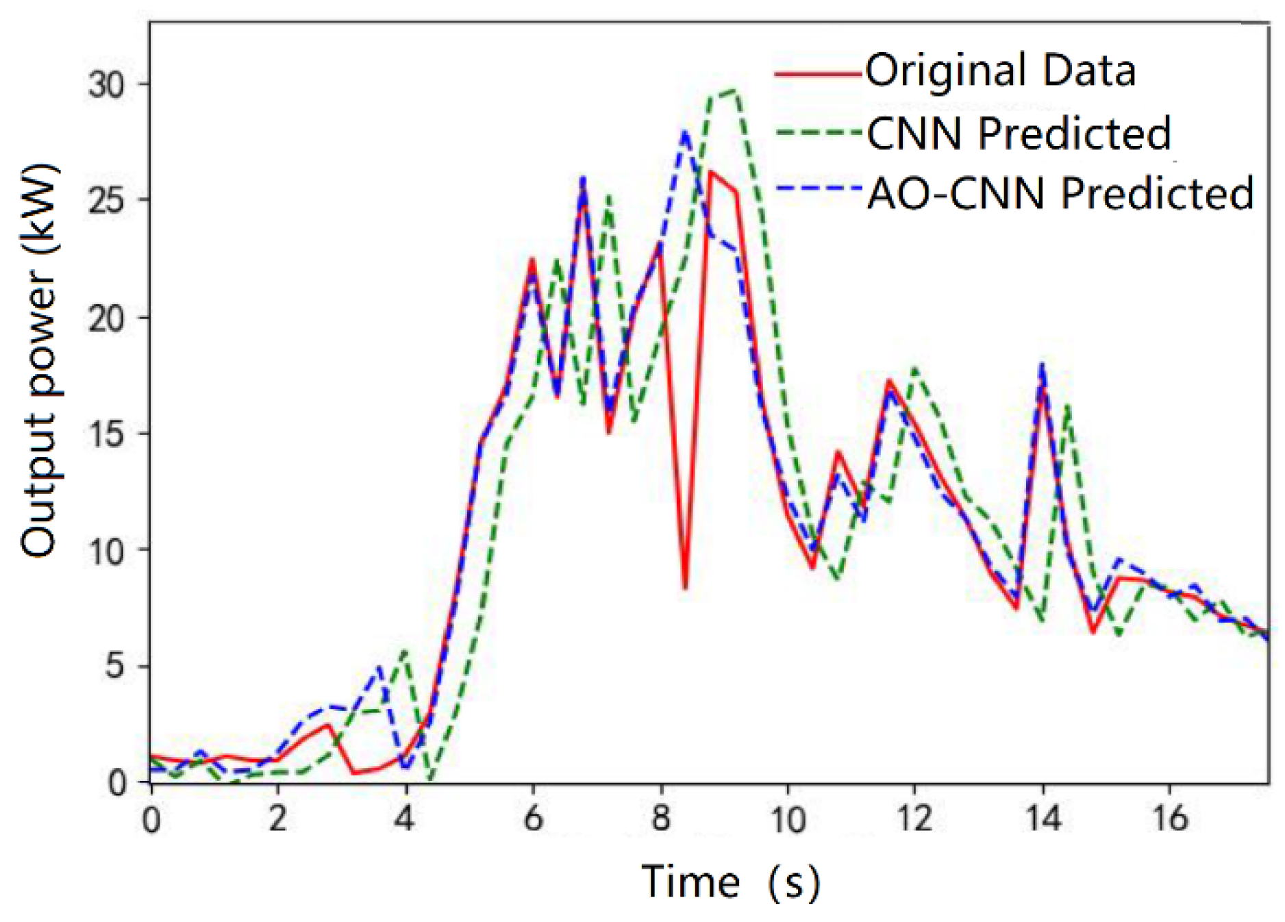
Figure 3 shows the spring model of the fitting graph, which is used to show the fitting effect of the CNN and AO-CNN models. The vertical axis on the left shows the difference between the true and predicted values. The horizontal axis represents photovoltaic power data in hours. The blue dotted line represents the predicted value of the AO-CNN model. The green dotted line represents the predicted value of the original CNN model, and the red line represents the true value. As can be seen from the figure, the two models are less affected by spring weather and both models fit the real value well, but the predicted value of the AO-CNN model is closer to the real value, and the difference is smaller. The AO-CNN model has a large deviation in the prediction value from the sample time of 8–9 h, which may be caused by data abnormality or model inadequacy.
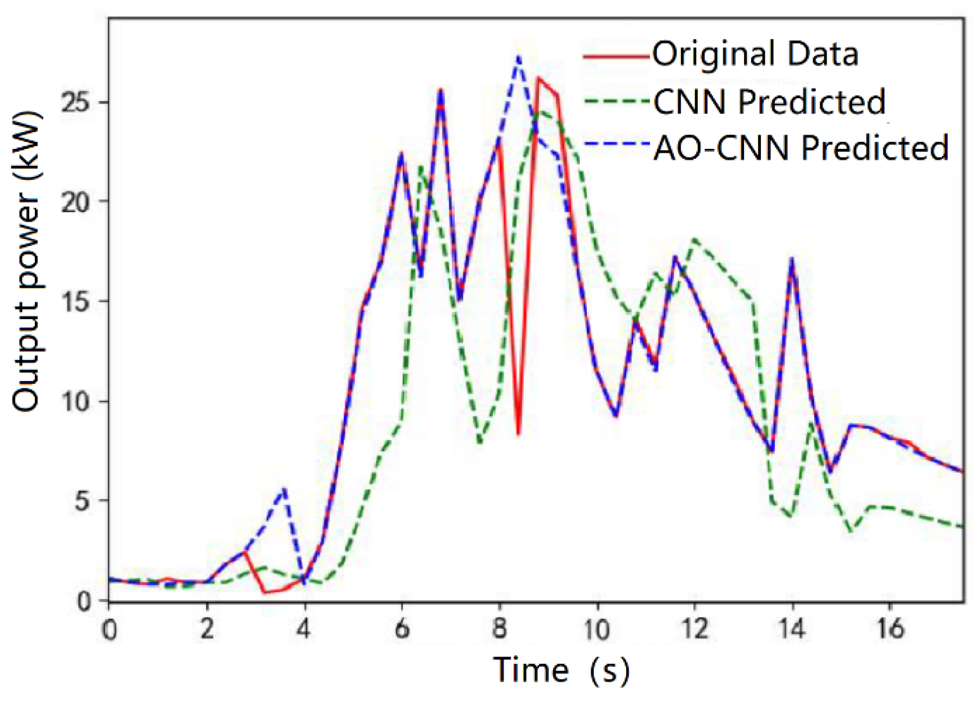
The summer model fitting diagram can be seen in Figure 4. It can be seen that the curve fluctuates greatly, and the two models are greatly affected by the weather in summer, which eventually leads to the green curve. The line deviates significantly from the original data, and the CNN model cannot properly match the true value. The purple curve basically coincides with the red curve. That is, the predicted value of the AO-CNN model proposed in this paper has a better fitting effect than that of the CNN model. The value is smaller. The predicted value of the AO-CNN model has a large deviation from 6–9 h in the sample time, which may be the actual number. It is also possible that the model was in error or did not fit, but overall, it is a better predictor of real data as there is better precision.
Figure 5 shows the fitting diagram of the model in the fall. It can be observed that the weather in autumn has less effect. The two models discussed in this paper closely fit the real values. Blue is the AO-CNN prediction curve, which is similar to the original data. That is, the curve of the red line is fitted more comprehensively, and the predicted value of the proposed AO-CNN model is higher than that of the CNN model, indicating that the fitting effect is better.
Figure 6 shows the winter fit of the model. It can be seen from the figure that the two models are affected by the winter weather, with the result that the CNN model does not match the real values well, but the forecast value of the AO-CNN model proposed in this paper is closer to the real values, with smaller differences. The predicted values of the AO-CNN model show a large deviation at the sample time from 8 to 9 h, which may be due to data anomalies or model underfitting.
Table 1 shows the differences between CNN and AO-CNN. It can be seen that the PV power prediction error of AO-CNN is smaller. Overall, the AO-CNN model performs better than the CNN model, demonstrating that the accuracy requirements of computer models can be further improved after the basic structure parameters of CNN model graphs are cleared by the deep learning algorithm based on group intelligence. The prediction effect of AO-CNN is better than that of the CNN model.

6. Photovoltaic Power Prediction Based on the IAO-LSTM Network

6.1. LSTM Neural Network

Although CNN is often used in actual photovoltaic power prediction, its performance in processing sequence data with time characteristics is not advantageous, and the accuracy of photovoltaic power prediction still needs to be further improved. Therefore, a neural network called Long Short-Term Memory (LSTM) was introduced, which has obvious superiority in time-series analysis. At the same time, because the Aquila optimization algorithm appearing in the global index search process is insufficient, a new improved Aquila optimization algorithm (IAO) is proposed. This algorithm is used to optimize the parameters of LSTM neural networks, and finally, the photovoltaic power prediction model of IAO-LSTM network is constructed. It is then verified with the database-related data mentioned above.
The LSTM LAN comprises several LSTM units, and the neurons in each layer are the same as those in BP deep neural network. The LSTM network is similar to the training of many neural networks in that its learning mode is also a backward propagation of error calculation law. Since the LSTM network is a network with a repetitive structure, its learning algorithm is also called backward propagation algorithm. Its learning process mainly includes two aspects: forward transfer and backward transfer. In LSTM neural network learning, the optimal solution has a great influence, and the most common one is the gradient descent method.

6.2. Improved Aquila Optimization Algorithm

In view of the problems of the existing standard AO algorithm, such as insufficient overall search ability and the tendency to fall into local extreme values, we attempt to improve the standard AO algorithm with the Cauchy mutation and other methods, and test it using four standard functions.
In the particle swarm optimization, the Cauchy variation coefficient is added. Specifically, the Cauchy variation method is proposed for the first specific iteration process to ensure that the algorithm can jump out of the optimal solution of local organization and try to find an optimal algorithm. The complex density function of the Cauchy distribution in standard three-dimensional space is shown as follows:
f ( x ) = 1 π 1 1 + x 2 < x <
Since the characteristic of the density function of the Cauchy distribution is that it does not cross the X axis, the random numbers produced may leave the origin. The formula for generating random numbers using the Cauchy distribution is as follows:
C a u c h y ( 0 , 1 ) = tan [ π ( ξ 1 2 ) ]
where ξ is random, less than 1 and greater than 0. The formula for updating the individual position of the Aquila by Cauchy mutation method is as follows:
X q + 1 = X q ( 1 + C a u c h y ( 0 , 1 ) )
where X q is the individual before the mutation, and X q + 1 is the individual after the mutation. Using the principle of survival of the fittest, the fittest values before and after mutation are compared to update the individual position.
Time complexity analysis usually includes three aspects: population initialization calculation fitness function, and updating the solution. It is assumed that the population number is N, the computational complexity of population initialization is O ( N ) , and the computational complexity of solution updating process is O ( T × N ) + O ( T × N × D ) , where T is the total number of iterations and D is the dimension of the problem.
Therefore, the total time complexity of the standard AO algorithm is O ( N × ( T × ( D + 1 ) ) ) . However, only the T distribution strategy O ( T × N ) is added to the IAO algorithm, without increasing the computational complexity, because the total time-interval complexity of the IAO algorithm is O ( N × ( T × ( D + 1 ) + 1 ) ) . The IAO algorithm has the same complexity as the traditional AO algorithm and does not add any additional level of operation.
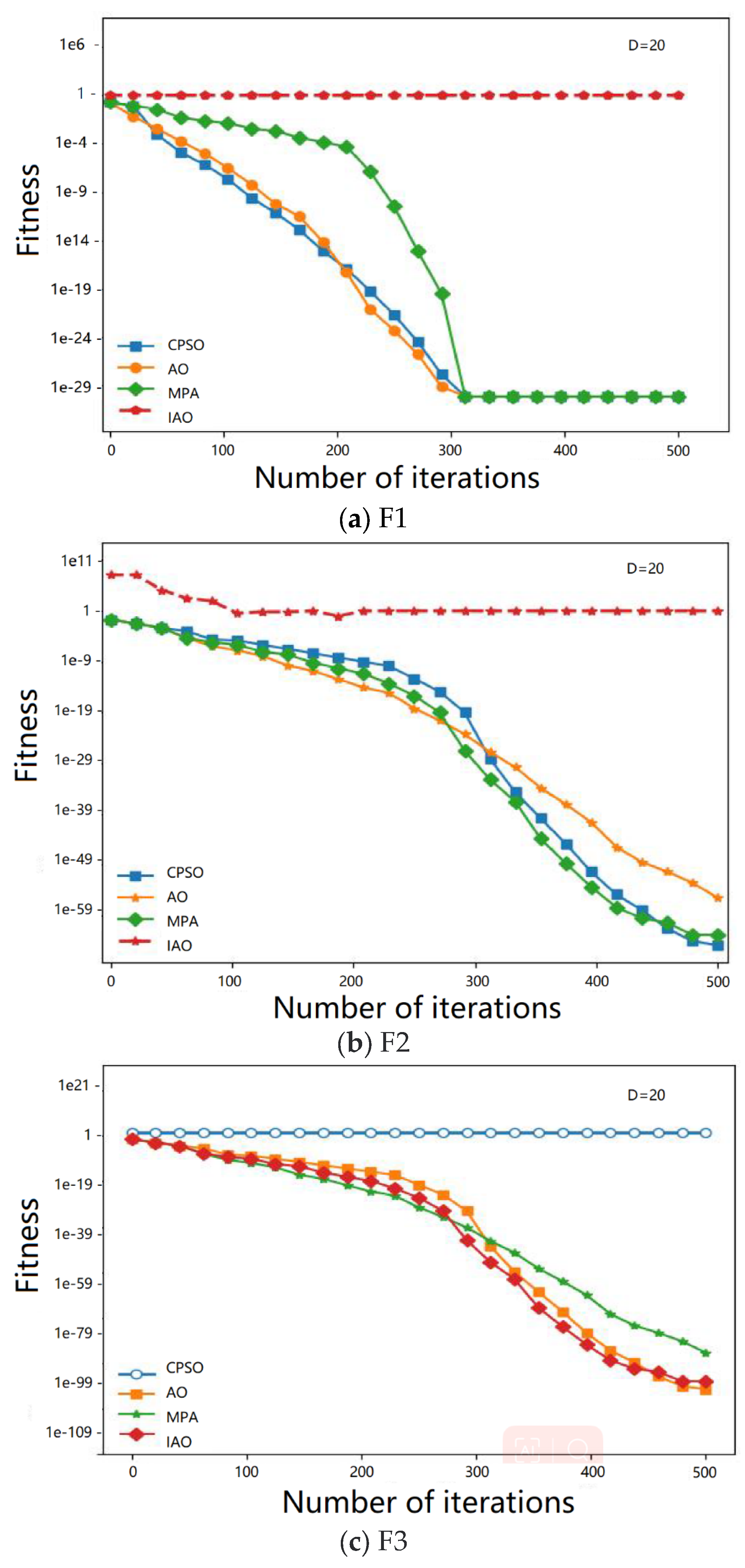
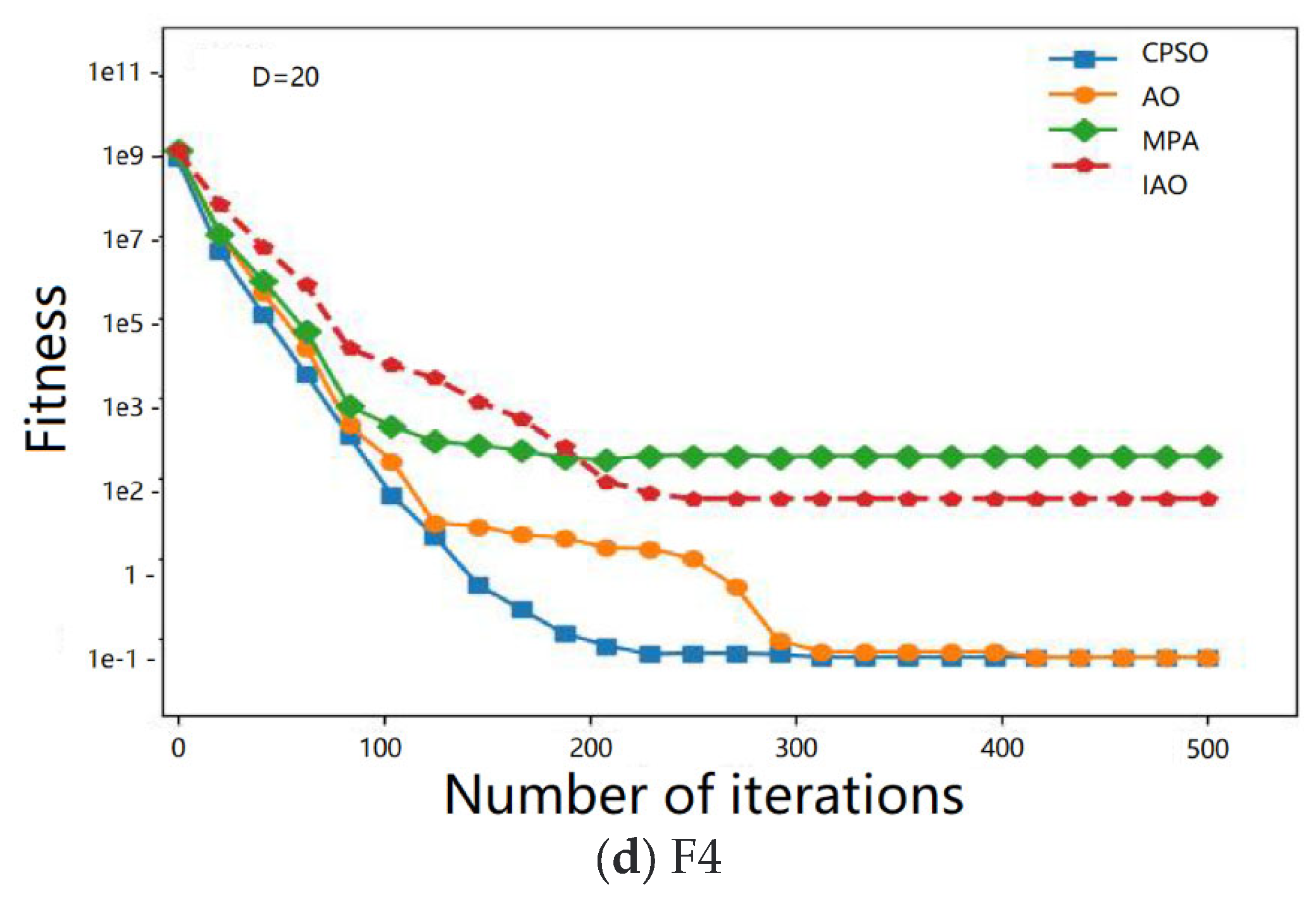
Four standard functions were selected, of which two were unimodal and two were multimodal, and their results were used to test the IAO performance. Table 2 presents the standard functions: F1 describes four standard functions, F1 to F2 are single mode functions, and F3 to F4 are multi-mode functions. For a single mode function, its search capability can be tested because it has a unique global optimal solution. The other part of the test composite function curve is shown in Figure 7.
Figure 7 shows a portion of the two-dimensional plane display images of the compound test function and the contraction change curves of various algorithms. Figure 7a–d display the digital F1, F2, F3 and F4 plane display images, respectively. In addition, F1 and F2 are single-peak composite functions, and there are only two optimal choices. F3 and F4 are complex multimodal functions with multiple optimal local fabric choices. It should be noted that the composite function of the selected cell is semicircular, but the smaller the final convergence, the faster the specific requirements are met.
The deep learning algorithm is used to compare the test results of each test compound function including the weighted average, probability distribution, optimal solution value, and difference value. The test results for the four benchmark functions are shown in Table 2. For all the combined F1-F2 functions of a single neural network, the AO algorithm performs better than the CPSO algorithm. The global optimal choice of the composite function for calculating F1-F2 elements is 0, but the optimal solution and weighted average of the AO and Marine Predators Algorithm (MPA) are not 0. The optimal solution values and weighted average of F1 and F2 are 0. For the composite function of a single neural network model, the test results of the F1-F2 test composite function all verify that the quality and performance of the proposed IAO are more competitive.
For composite functions F3 and F4, the final linear distance test of the CPSO algorithm is expected to have a large final large gap. When testing the composite function F4, IAO’s optimal solution value is the best choice for calculating the closest test composite function in the deep learning algorithm. In both algorithms, the final value of IAO is closer to the expected value. Through the testing of F3 and F4, it is found that the optimization potential of IAO is relatively better than other specific methods. In general, often according to the above analysis, most single neural network model composite functions are still composite functions of natural language understanding. Compared with AO and its improved MPA, IAO is more competitive, stable and secure. Finally, it is shown that after the improvement of the computing unit AO with the help of the Cauchy mutation and other operational strategies, IAO has relatively effective computing and development potential, and IAO has stronger global optimization potential.

6.3. The Short-Term Photovoltaic Power Prediction Model of the IAO-LSTM Network

The LSTM network has a good ability to predict time series. However, the structure and modeling accuracy of LSTM networks depend on the selection of their hyperparameters, which directly affect the prediction effect of LSTM networks. At present, hyperparameter selection in the LSTM network mainly relies on prediction and many experiments. This is not only inefficient, but it is also difficult to obtain reasonable hyperparameter values. Here, in the context of machine learning, hyperparameters are parameters whose values are set before the learning begins, rather than parameter data obtained through training. Under normal circumstances, hyperparameters are optimized to select a group of optimal hyperparameters for the learning machine to improve the performance and effect of learning. Therefore, hyperparameters are derived from human experience and are subject to hardware constraints. On this basis, the IAO method is proposed to optimize the key parameters in the LSTM network and improve the accuracy of LSTM network modeling. Hyperparameters have a great influence on the prediction ability of LSTM networks. Improper selection leads to a decline in the prediction capacity of the LSTM network. In LSTM, the number of hidden layer neurons and the interval of reinforcement training batches are two indispensable related parameters which hinder the overall quality and performance of LSTM. Increasing the number of hidden layer neurons in LSTM neural networks can improve their fitting performance and prediction accuracy.
As the number of neural networks increases, the need for computation also increases, and the learning speed of neural networks is affected to some extent. Each neural network can be used to describe the training batch and time interval of intensive training, but further improving the training batch time interval of neural network intensive training can effectively further improve computing power. It can also further improve the memory utilization efficiency of the operating system and shorten the product iteration cycle. However, in specific cases where the same training batch has improved significantly, database overflows, software program crashes, and so on can occur. If the appropriate parameters are selected, not only can the learning speed of motion be accelerated, but also the accuracy of 3D images can be further improved to avoid the possibility of generalization ability and other problems being difficult to solve.
In this paper, a new and improved IAO algorithm for Aquila deep learning is adopted. By testing the composite function, the aim was to verify the quality and performance of the IAO cell, thereby enabling the continuous improvement of the two new and current effective algorithm models. This testing indicates that IAO has good optimization potential. IAO was selected to optimize LSTM local area network (LAN) connectivity parameters, the number of hidden layer neurons, and the time interval of connection reinforcement training batches, in order to promote IAO automatic convergence in hyperparameters and optimize LSTM connectivity correlation. Thus, IAO can optimize the LSTM connection parameters.
Determining the number of hidden layer neurons enables us to optimize the LSTM LAN connection and further enhance the training batch time interval. The overall optimal choice is to allow the target compound function to obtain the corresponding value range of Aquila-related parameters, where the Aquila position in the vector space of the number of neurons in the time interval between the hidden layer and the reinforcement training batch corresponding to the LSTM neural network prediction model error is less than one. With IAO, the LSTM connection parameters can be automatically optimized to avoid measurement errors caused by manual selection of relevant parameters. IAO-LSTM makes basic connections based on LSTM neural networks. The optimal number of hidden layer neurons and the interval of intensive training batches were used as parameters for LSTM neural network connection.
The basic steps of the IAO-LSTM network model optimization process are:
Step 1: The relevant LSTM connection parameters are initialized. Then, the basic framework of LSTM connectivity and its related parameters are preliminarily preprocessed and inputted into the IAO-LSTM connectivity training set.
Step 2: The optimal IAO parameters are initialized. The population number, iteration times and other parameters are set. We then take the optimal LSTM network model as the optimal Skyhawk individual, and take the error function in the algorithm network model as the optimal fitness.
Step 3: Based on the number of training batches of the LSTM network and the number of neurons in the hidden layer, each Aquila is positioned and trained with the initial parameters to obtain the adaptive value of the Aquila (training error of the LSTM network), and then compared with the adaptive value of each individual to find the optimal search subject.
Step 4: The IAO correction formula is used to correct and determine the Aquila’s position. On this basis, genetic algorithms are used to solve the algorithm. Otherwise, the number of optimal individuals and the size of the optimal adaptation value are maintained.
Step 5: When the maximum number of iterations is reached, the iteration is terminated to obtain the optimal solution. Otherwise, the model returns to step 4 and continues looking for the best individual.
Step 6: The relevant parameters in the IAO from the optimal individual scheme location are decoded. Then the relevant parameters considered most suitable for the LSTM connection are decoded.
Step 7: After garbage file cleaning, the LSTM neural network is intensively trained using the deep learning model. Then the test data set is selected to predict the nominal photovoltaic output power, and finally the prediction is recorded.
Through the construction and optimization of the IAO-LSTM network model, the photovoltaic power prediction mechanism is further understood. However, the existing IAO-LSTM neural network model cannot train and predict the entire system. Specifically, the actual photovoltaic power generation has a certain seasonal variation so it needs to be pretreated. According to the actual situation, the prediction model suitable for the data set is established. The distributed PV active power database data and their corresponding meteorological database data are determined. Then, the deep learning model is further divided into four parts. The deep learning model can be divided into spring, summer, autumn, and winter according to the physical characteristics of spring and autumn. After the deep learning model is preprocessed, the number of selected parameters in the IAO-LSTM sub-deep learning model is cleaned with the help of the enhanced training set, and then the actual power output data of photovoltaic power generation is predicted by continuing to select the test set.

6.4. Model Verification

The model evaluation indices used in this paper were the mean root square error (RMSE) and mean absolute error (MAE). When using the same database data as the AO-CNN prediction model above for model verification, the selected database data had to be relatively stable. Only on this basis could the results be compared. In order to make comparisons and draw differences, the predictive power of the proposed PV statistical model needs to be verified and the LSTM and AO-LSTM of the computing element compared.
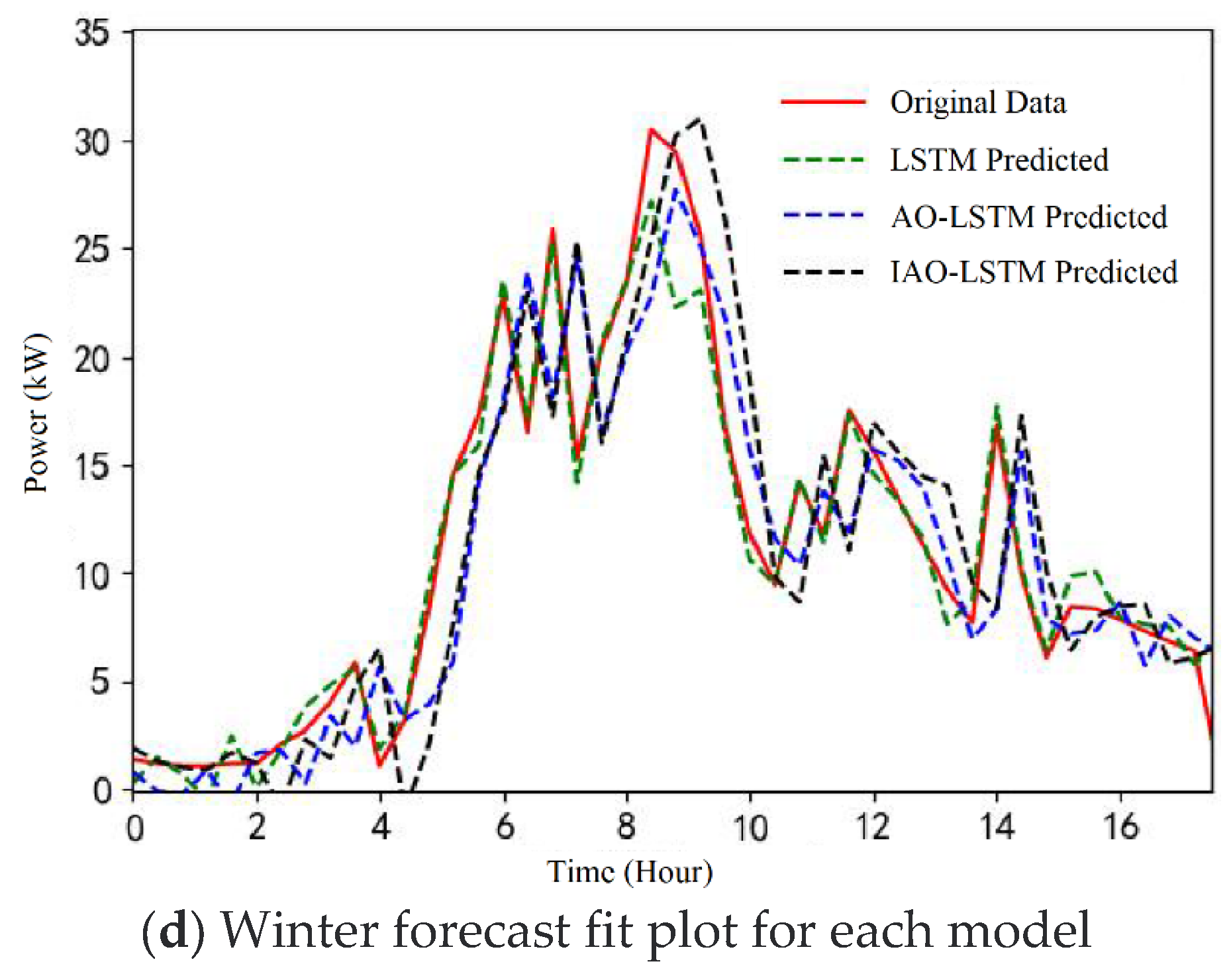
The interval of intensive training for all images was set to 200 times. The image of LAN connection uses MSE as the activation function. The value of genetic diversity of the deep learning algorithms was set to 30, and the product iteration interval of deep learning algorithms was 20 times. Through the deep learning models and tests, the actual photovoltaic power could be predicted. Finally, AO-CNN and its comparison graphs were used to predict the rated photovoltaic output power, and the different prediction effects are shown in Figure 8a–d. The figure shows the prediction effects of the LSTM, AO-LSTM, and IAO-LSTM models after fitting the data for four seasons. The left vertical axis shows the difference between the true and predicted values, and the horizontal axis shows the PV power data time in hours. The green dotted line represents the prediction result of the LSTM model, the blue dotted line represents the prediction result of the original AO-LSTM model, the black dotted line represents the prediction result of the IAO-LSTM model, and the red solid line represents the true value.
As can be seen in Figure 8, the red and black lines tend to be more similar. Compared with the LSTM model and the AO-LSTM model, the IAO-LSTM model can better fit the true values, and the difference is small. There is a large deviation in the predicted values of the LSTM model in the 8–10 h of sample time range, which may be caused by abnormal data processing. Simply comparing the calculated PV active power curve with the reference curve cannot quantify the chart quality or visually evaluate its relative effect, so the error values are used to assess the results. Table 3 lists the values of the LSTM model, AO-LSTM model, and IAO-LSTM comparison model in terms of RMSE and MAE in four seasons. Comparing the error values of the LSTM, AO-LSTM and IAO-LSTM models in Table 3, it is clear that IAO-LSTM has higher accuracy in photovoltaic power prediction.
In conclusion, the experimental results show that the IAO-LSTM photovoltaic power prediction model proposed in this paper has smaller errors in all four seasons, and its overall quality and performance are better than that of LSTM and AO-LSTM. Compared with the AO-CNN model mentioned above, the performance of the IAO-LSTM model is also a significant improvement.

7. Conclusions

With the increase in the penetration rate of new energy, it is necessary to improve the ability of new energy to participate in the frequency regulation and voltage regulation of the power grid. However, the current energy storage technology is not mature in terms of safety, and the cost performance is low. To enable its participation in frequency regulation and voltage regulation of the power grid, it is necessary to accurately predict the output of the new energy field. This paper analyzes and studies the common methods of photovoltaic electric field output power prediction models, such as the CNN and AO algorithms, and the AO-CNN, LSTM and AO-LSTM models, etc. After comparing and analyzing the advantages and disadvantages of these models, we propose using IAO to optimize LSTM neural network parameters and establish a model for predicting actual photovoltaic power. The proposed IAO-LSTM model was applied in the field of photovoltaic power prediction. The experimental results show that the IAO-LSTM photovoltaic power prediction model has less error and that its overall quality and performance are better than the other abovementioned prediction models. In the future, if the proposed method can be combined with load forecasting, it will be able to accurately determine the frequency modulation region and adopt frequency modulation means to realize a supporting role in the power grid.

Author Contributions

Writing—review and editing, L.L.; writing—original draft preparation, Y.L.; All authors have read and agreed to the published version of the manuscript.

Funding

This work was financially supported by the Basic Research Surface Projects of Shanxi Province (202203021221153).

Data Availability Statement

Which will be found in Weipu net in future.

Acknowledgments

The authors acknowledged the financial support from Basic Research Surface Projects of Shanxi Province (202203021221153).

Conflicts of Interest

The authors declare no conflict of interest.

References

  1. Yang, D.; Kileissl, J.; Gueymard, C.A.; Pedro, H.T.; Coimbra, C.F. History and trends in solar irradiance and PV power forecasting: A preliminary assessment and review using text mining. Sol. Energy 2018, 168, 60–101. [Google Scholar] [CrossRef]
  2. Ma, T.; Yang, H.X.; Lin, L. Solar photovoltaic system modeling and performance prediction. Renew. Sustain. Energy Rev. 2014, 31, 75–83. [Google Scholar] [CrossRef]
  3. Li, Y.T.; Su, Y.; Shu, L.J. An ARMAX model for forecasting the power output of a grid connected photovoltaic system. Renew. Energy 2014, 66, 820–823. [Google Scholar] [CrossRef]
  4. Persson, C.; Bacher, P.; Shiga, T.; Madsen, H. Multi-site solar power forecasting using gradient boosted regression trees. Sol. Energy 2017, 150, 820–823. [Google Scholar] [CrossRef]
  5. Ruby, N.; Jayabarathi, R. Predicting the Power Output of a Grid-Connected Solar Panel Using Multi-Input Support Vector Regression. Procedia Comput. Sci. 2017, 115, 75–83. [Google Scholar]
  6. Li, Y.Z.; Niu, J.C.; Li, L. Forecast of Power Generation for Grid-Connected Photo-voltaic System Based on Grey Theory and Verification Model. Energy Power Eng. 2013, 5, 177–181. [Google Scholar] [CrossRef]
  7. Wang, H.; Yi, H.; Peng, J.; Wang, G.; Liu, Y.; Jiang, H.; Liu, W. Deterministic and probabilistic forecasting of photovoltaic power based on deep convolutional neural network. Energy Convers. Manag. 2017, 153, 409–422. [Google Scholar] [CrossRef]
  8. Rodríguez, F.; Fleetwood, A.; Galarza, A.; Fontán, L. Predicting solar energy generation through artificial neural networks using weather forecasts for microgrid control. Renew. Energy 2018, 126, 855–864. [Google Scholar] [CrossRef]
  9. Yan, A.Y.; Gu, J.B.; Mu, Y.H.; Li, J.; Jin, S.; Wang, A. Research on photovoltaic ultra short-term power prediction algorithm based on attention and LSTM. IOP Conf. Ser. Earth Environ. Sci. 2021, 675, 151–158. [Google Scholar] [CrossRef]
  10. Bruni, V.; Della Cioppa, L.; Vitulano, D. An automatic and parameter-free information-based method for sparse representation in wavelet bases. Math. Comput. Simul. 2020, 176, 73–95. [Google Scholar] [CrossRef]
  11. Koster, D.; Minette, F.; Braun, C.; O’Nagy, O. Short-term and regionalized photovoltaic power forecasting, enhanced by reference systems, on the example of Luxembourg. Renew. Energy 2019, 132, 455–470. [Google Scholar] [CrossRef]
  12. Hafeez, G.; Alimgeer, K.S.; Khan, I. Electric load forecasting based on deep learning and optimized by heuristic algorithm in smart grid. Appl. Energy 2020, 269, 114915. [Google Scholar] [CrossRef]
  13. Ge, Q.B.; Guo, C.; Jiang, H.Y.; Lu, Z.; Yao, G.; Zhang, J.; Hua, Q. Industrial power load forecasting method based on reinforcement learning and Psolssvm. IEEE Trans. Cybern. 2022, 52, 1112–1124. [Google Scholar] [CrossRef] [PubMed]
  14. Du, P.; Wang, J.Z.; Yang, W.D.; Niu, T. Multi-step ahead forecasting in electrical power system using a hybrid forecasting system. Renew. Energy 2018, 122, 533–550. [Google Scholar] [CrossRef]
  15. Kong, W.C.; Dong, Z.Y.; Jia, Y.W.; Hill, D.J.; Xu, Y.; Zhang, Y. Short-term residential load forecasting based on LSTM recurrent neural network. IEEE Trans. Smart Grid 2019, 10, 841–851. [Google Scholar] [CrossRef]
  16. Ozawa, A.; Furusato, R.; Yoshida, Y. Determining the relationship between a household’s lifestyle and its electricity consumption in Japan by analyzing measured electric load profiles. Energy Build. 2016, 119, 200–210. [Google Scholar] [CrossRef]
  17. Wang, H.; Qi, L.H.; Yan, L.; Li, Z. Load photo: A novel analysis method for load data. IEEE Trans. Smart Grid 2021, 12, 1394–1404. [Google Scholar] [CrossRef]
  18. Ye, C.J.; Ding, Y.; Wang, P.; Lin, Z. A data-driven bottom-up approach for spatial and temporal electric load forecasting. IEEE Trans. Power Syst. 2019, 34, 1966–1979. [Google Scholar] [CrossRef]
  19. Al-Wakeel, A.; Wu, J.Z.; Jenkins, N. K-means based load estimation of domestic smart meter measurements. Appl. Energy 2017, 194, 333–342. [Google Scholar] [CrossRef] [Green Version]
  20. Muthu Kumar, B.; Maram, B. AACO: Aquila Anti-Coronavirus Optimization-Based Deep LSTM Network for Road Accident and Severity Detection. Int. J. Pattern Recognit. Artif. Intell. 2023, 37, 2252030. [Google Scholar]
  21. Mohammed, A.A.A.; Ahmed, A.E.; Fan, H.; Ayman Mutahar, A.; Mohamed, A.E. Modified aquila optimizer for forecasting oil production. Geo-Spat. Inf. Sci. 2022, 25, 519–535. [Google Scholar]
  22. Li, Z.; Luo, X.; Liu, M.; Cao, X.; Du, S.; Sun, H. Short-term prediction of the power of a new wind turbine based on IAO-LSTM. Energy Rep. 2022, 8, 9025–9037. [Google Scholar] [CrossRef]
  23. Huang, Y.; Jiang, H. Soil Moisture Content Prediction Model for Tea Plantations Based on a Wireless Sensor Network. J. Comput. 2022, 33, 125–134. [Google Scholar] [CrossRef]
Figure 1. Schematic diagram of convolutional neural network model.
Processes 11 01957 g001
Figure 2. Schematic diagram of convolutional calculation.
Processes 11 01957 g002
Figure 3. Spring forecast fit plot for each model with traditional methods.
Processes 11 01957 g003
Figure 4. Summer forecast fit plot for each model with traditional methods.
Processes 11 01957 g004
Figure 5. Autumn forecast fit plot for each model with traditional methods.
Processes 11 01957 g005
Figure 6. Winter forecast fit plot for each model with traditional methods.
Processes 11 01957 g006
Figure 7. Two-dimensional function convergence curve.
Processes 11 01957 g007aProcesses 11 01957 g007b
Figure 8. Season forecast fit plot of each model.
Processes 11 01957 g008aProcesses 11 01957 g008b
Table 1. Season forecast error table for each model with traditional methods.
SeasonError TypeCNNAO-CNN
SpringRMSE (%)2.141.83
MAE (%)4.952.90
MAPE(%)1.253.84
SummerRMSE (%)2.001.75
MAE (%)3.072.68
MAPE(%)5.025.11
AutumnRMSE (%)1.491.25
MAE (%)2.762.24
MAPE(%)6.566.88
WinterRMSE (%)1.200.89
MAE (%)2.721.60
MAPE(%)6.918.39
Table 2. Four benchmark functional test functions.
FunctionsExpressionSearch SpaceDimensionOptimal Solution
F1 F ( x ) = k = 1 D x k 4 + r a n d ( 0 , 1 ) [−200,200]300
F2 F ( x ) = k = 1 D x k 2 [−2.28,2.28]300
F3 F ( x ) = k = 2 D ( 10 6 ) ( k 1 ) ( D 1 ) x k 2 [−22,22]300
F4 F ( x ) = k = 1 11 [ a k x 1 ( b k 2 + b k x 2 ) b k 2 + b k x 3 + x 4 ] 2 [−40,40]300
Table 3. Season forecast error table for each model.
SeasonError TypeLSTMAO-LSTMIAO-LSTM
SpringRMSE (%)1.871.481.38
MAE (%)2.671.761.91
MAPE (%)1.323.846.56
SummerRMSE (%)1.841.080.91
MAE (%)2.921.661.29
MAPE (%)4.616.386.31
AutumnRMSE (%)0.900.840.71
MAE (%)1.131.260.84
MAPE (%)7.766.887.47
WinterRMSE (%)1.010.710.61
MAE (%)1.431.150.91
MAPE (%)6.918.395.02
Disclaimer/Publisher’s Note: The statements, opinions and data contained in all publications are solely those of the individual author(s) and contributor(s) and not of MDPI and/or the editor(s). MDPI and/or the editor(s) disclaim responsibility for any injury to people or property resulting from any ideas, methods, instructions or products referred to in the content.