Abstract
This study presents a Simulink model and the simulation of a central water cooling system and the main seawater pump motor of a 59,990 DWT bulk carrier, based on a direct torque control strategy to control the frequency of the ship’s water cooling pump motors. Simulation curves of the water cooling system under different sailing conditions were simulated based on 100% of rated power, 80% of common power, and the seawater temperature of the ship’s main engine. The simulation of the current, speed, and torque of the pump motor under direct torque control verified that the ship’s water cooling pump motor could save approximately 22.70%, 36.76%, and 52.70% of electrical energy, respectively, throughout the year with this inverted control solution.
1. Introduction
At present, in international trade, whether we are discussing land transport, water transport, or air transport, “green transport” has become a consistent goal. In a ship’s traditional central water cooling system, the design and size of the pump are to ensure the safety of the system and select the maximum capacity of the supporting facilities. The pump always runs at rated power, and the cooling load of the main engine is poorly matched under varying working conditions, resulting in much energy being wasted [1].
It is a matter of urgency to study energy conservation and measures for reducing emissions by ships [2]. The energy consumption of marine water cooling pumps accounts for 65–70% of the entire central water cooling system [3], so the study of the energy savings during the operation of a water cooling pump has important application value. Kocak et al. [4] proposed that the load of the seawater cooling system depends on parameters such as the seawater’s temperature and the generator’s load. By comparing the energy-saving effects of a pump with a constant speed and one with a variable speed, they concluded that the system with a VFD pump could save a large amount of fuel and costs at different seawater temperatures.
Dere et al. [5] quantified the energy-saving effects of the main engine cooling system by using a real cabin simulator of a container ship with a waste heat recovery system, and their study showed that the use of variable-speed pumps could reduce about 60% of the power consumption and 80% of the fuel consumption. Zhang et al. [6] took the marine water pump model “RVA-280JN” as their research object, conducted a simulation on a real ship, and designed a variable rheological pressure control curve that had obvious energy-saving effects on the central water cooling system of the ship and had advantages such as high reliability, fast cooling, and rapid feedback.
These methods can effectively calculate the energy consumption of marine cooling pump motors and provide some insights for marine energy-saving strategies. However, when these methods were compared from an economic point of view, it was found that the investment in retrofitting the cooling pump with variable frequency control systems far exceeded the return on fixed-speed pumping systems. Since the response speed and dynamic smoothness of the pump motor was not studied, the reliability of the system was not verified.
There have also been some authors who have studied the frequency control process of motors and have achieved some results. Chinmaya et al. [7] pointed out the advantages of the direct torque control method, namely, that it does not require any complex control algorithm, and uses simple commands for controlling the induction motor’s flux and torque. They modeled and simulated the direct torque control of asynchronous motors in MATLAB/Simulink, and tested it successfully by checking parameters such as the stator’s current d and q, and the flux, speed, and torque of the d and q axis. The experimental results showed that the DTC model has a good dynamic response to the change in the demand torque in terms of the response of speed. Jafari et al. [8] proposed an improved matrix converter-driven direct torque control switching table for two parallel asynchronous motors. Its mean-based control strategy allowed all the switching states of a matrix converter to be used and studied, and, ultimately, the optimal switching state to be selected from among them. The experimental results showed that compared with the traditional method, the overshoot of a change in the motor’s speed was reduced by 1%, and the electromagnetic torque oscillation was also reduced, which proved the advantages of the DTC algorithm and applied it to a matrix converter. Li [9] first built a mathematical model for the motor of a ship’s main pump and established the equations of the motor’s flux linkage, voltage, electromagnetic torque, and motion. The inverted state was studied, and the direct torque control system model of the main pump motor in a marine central water cooling system was established. The results showed that the variable-frequency speed regulation of the ship’s main pump based on DTC had a good dynamic response and effectively reduced the energy consumption of the pump.
Although existing studies have been conducted on controlling a pump’s frequency in marine central water cooling systems, they have mainly focused on modeling and simulating the entire system. There is no complete model of the motor, nor is there a more detailed division of the operation cycle of the inverted pump motor. On the basis of the previous research on the conversion method of controlling a pump’s frequency, this study analyzed the dynamic response effects of the 12-sector division of the operating cycle of the frequency converter of a marine cooling pump motor. The energy-saving effects of a marine central water cooling system based on the direct torque control method was studied. Simulink was used to model and simulate the central water cooling system of a ship, and the direct motor torque control method could achieve a good dynamic response of the inverted control system. The simulation results showed that the control system could significantly reduce the energy consumption of the cooling pump motor.
2. Marine Central Water Cooling System
To obtain accurate simulation results, the complete cooling principle of a ship’s central water cooling system needed to be mastered. The schematic diagram of the seawater cooling system for a 59,990 DWT bulk carrier is shown in Figure 1. As can be seen from the diagram, when the system is started and the seawater pump starts working, the seawater is drawn into the pipeline and flows to the central water cooling system and exchanges heat with the high-temperature freshwater. This results in the cooling of the hot freshwater, which is eventually discharged off-board through the piping.
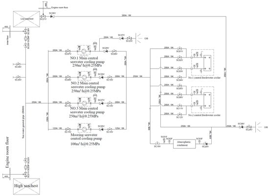
Figure 1.
Schematic diagram of the seawater cooling system.
Figure 2 shows the schematic diagram of the freshwater cooling system for a 59,990 DWT bulk carrier. As can be seen from the diagram, when the system is started, the low-temperature freshwater cooling pumps start working and the high-temperature freshwater first passes through the central cooler to exchange heat with the seawater. The seawater removes the heat from the water, thus cooling down the high-temperature freshwater to low-temperature freshwater, which then flows to the main engine’s air cooler and the main engine’s oil cooler via the pipeline. After cooling the hot high-pressure air and the high-temperature lubricating oil, the freshwater flows to the cylinder liner of the water cooler of the main engine and cools down the high-temperature freshwater in it. The ship’s central water cooling system is an important system for the safe navigation of the ship, so it is particularly important for each piece of equipment to be cooled in a timely fashion.
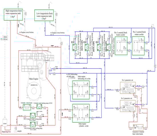
Figure 2.
Schematic diagram of the freshwater cooling system.
3. Simulation Model of a Ship’s Central Water Cooling System
3.1. Simulink Model of the Central Water Cooling System
The central water cooling system of a ship includes several subsystems, and the system is very complex. This study therefore first modeled each submodule individually and then linked the modules together to finalize the model of the whole system. In the central water cooling system of a ship, the main heat load devices are the main engine’s cylinder liner, the cylinder liner of the water cooler, the main engine’s slip oil cooler, the main engine’s air cooler, the auxiliary engine’s cooler, and other components to be cooled.
In Figure 3, Input 1 is the actual power share of the main engine, Input 2 is the cylinder liner for cooling the main engine’s temperature, and Output 1 is the temperature of the high-temperature freshwater at the main engine’s outlet.

Figure 3.
Heat transfer simulation model of the main engine’s cylinder liner.
The heat transfer simulation model of the cylinder liner of the water cooler of the main engine is shown in Figure 4.
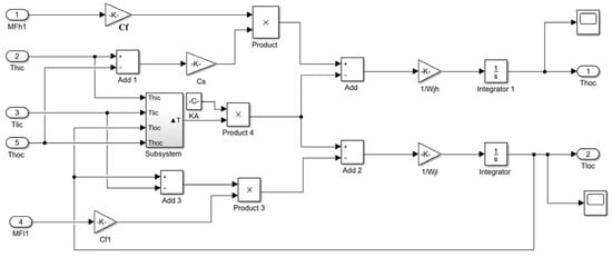
Figure 4.
Heat transfer simulation model of the cylinder liner of the water cooler of the main engine.
In this figure, Input 1 is the temperature of the low-temperature freshwater leaving the sleeve of the water cooler, Input 2 is the temperature of the high-temperature freshwater entering the sleeve of the water cooler, Input 3 is the mass flow rate of the low-temperature freshwater entering the sleeve of the water cooler, Input 4 is the mass flow rate of the high-temperature freshwater entering the sleeve of the water cooler, Output 1 is the temperature of the low-temperature freshwater leaving the sleeve of the water cooler, and Output 2 is the temperature of the high-temperature freshwater leaving the sleeve of the water cooler.
The simulation model of the high-temperature freshwater catchment is shown in Figure 5.
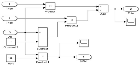
Figure 5.
Simulation model of the high-temperature freshwater catchment.
In the figure, Input 1 is the temperature of the high-temperature freshwater leaving the cylinder liner of the water cooler, Input 2 is the temperature of the high-temperature freshwater leaving the mainframe, Input 3 is the three-way valve opening of the high-temperature freshwater, Output 1 is the mass flow of the high-temperature freshwater entering the cylinder liner of the water cooler, and Output 2 is the temperature of the high-temperature freshwater entering the mainframe.
The simulation model of the high-temperature freshwater system is shown in Figure 6.
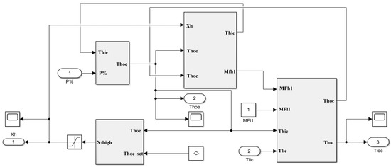
Figure 6.
Simulation model of a high-temperature freshwater system.
In this figure, Input 1 is the actual power share of the main engine, Input 2 is the temperature of the cold freshwater entering the cylinder liner of the water cooler, Output 1 is the opening of the three-way valve of the high-temperature freshwater, Output 2 is the temperature of the high-temperature freshwater leaving the main engine, and Output 3 is the temperature of the cold freshwater leaving the cylinder liner of the water cooler.
The simulation model of the main engine’s oil cooler is shown in Figure 7.

Figure 7.
Simulation model of the main engine’s oil cooler.
In this figure, Input 1 is the temperature of the cooled freshwater into the main engine’s oil cooler, Input 2 is the actual power share of the main engine, and Output 1 is the temperature of the main engine’s oil cooler at the freshwater cooling system.
The simulation model of the main air cooler is shown in Figure 8.

Figure 8.
Simulation model of the main air cooler.
In this figure, Input 1 is the temperature of the cold freshwater entering the main air cooler, Input 2 is the actual power share of the main air cooler, Output 1 is the temperature of the charged air leaving the main air cooler, and Output 2 is the temperature of the cold freshwater leaving the main air cooler.
The simulation model of the auxiliary cooler is shown in Figure 9.
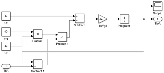
Figure 9.
Simulation model of the auxiliary cooler.
In this figure, Input 1 is the temperature of the cold freshwater entering the auxiliary cooler, and Output 1 is the temperature of the cold freshwater leaving the auxiliary cooler.
By combining these submodule systems, we obtained a simulation model of a frequency-controlled low-temperature freshwater cooling system, as shown in Figure 10.
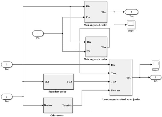
Figure 10.
Simulation model of the low-temperature freshwater cooling system.
In this figure, Input 1 is the actual power share of the main engine, Input 2 is the temperature of the cold freshwater leaving the cylinder liner of the water cooler, Input 3 is the temperature of the cold freshwater leaving the three-way valve of the cold freshwater, Output 1 is the temperature of the slip oil cooler in the cold freshwater system, and Output 2 is the temperature of the cold freshwater entering the central cooler.
The simulation model of the central cooler in inverted mode for the seawater system is shown in Figure 11.
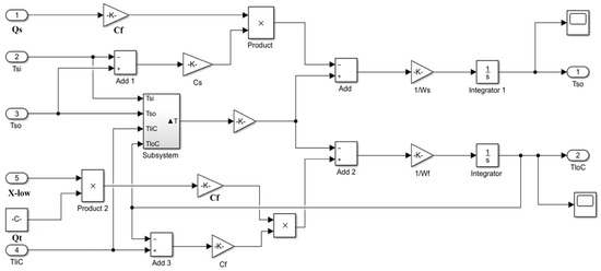
Figure 11.
Simulation model of the central cooler in variable-frequency mode.
In this figure, Input 1 is the flow rate of seawater drawn in by the seawater pump, Input 2 is the current temperature of the seawater, Input 3 is the temperature of the seawater discharged from the ship, Input 4 is the temperature of the cold freshwater at the inlet of the central cooler, Input 5 is the opening of the three-way valve of the cold freshwater, and Output 1 is the temperature of the cold freshwater at the central cooler’s outlet.
3.2. Simulink Model of the Motor with a Direct Torque Control System
The water cooling pumps in a ship’s central water cooling system generally use three-phase AC asynchronous motors. To achieve a fast and smooth response from the three-phase asynchronous motors, direct torque control methods are required. In this study, based on the basic principle of direct torque control, the direct torque control system for a ship’s water cooling pump motors was modeled and the system was simulated, thus verifying that the method could achieve a good dynamic response of the ship’s water cooling pump motors.
Direct torque control consists of two basic components: the torque control loop and the speed control loop. The DTC method uses the space vector method to analyze the mathematical model of an AC motor directly in the stator’s static mass coordinate system, to construct an algorithmic model of the torque and magnetic chain, and to calculate and control the torque of the AC motor. The PWM signal is generated with the help of a hysteresis loop controller to optimally control the switching state of the inverter directly via the switching table, thus achieving the high dynamic performance of the torque. Due to the constant switching of the voltage state, the trajectory of the stator’s magnetic chain approaches a circle and the interpolation of the zero voltage vector is used to change the frequency of the differential rotation in order to control the torque of the motor and its rate of change, thus enabling rapid changes in the magnetic chain and torque of the AC motor as required [10].
In this study, a mathematical model of the seawater pump motor was built under ideal conditions (i.e., only the main electromagnetic relationships in it were considered, without considering other factors that have less influence). The voltage equation, the magnetic chain equation, and the torque equation are shown below [11].
- (1)
- Voltage equation
- (2)
- Magnetic chain equation
- (3)
- Torque equation
The direct torque control system uses a two-position bang-bang controller, which simplifies the structure of the controller by using the two control signals, namely, the torque and magnetic chain, directly in the PWM inverter. The stator’s chain was selected as the controlled quantity, so it was not affected by changes in the rotor’s parameters, and a fast torque response could be obtained during the dynamic process of acceleration and deceleration or changes in the load of the system.
As shown in Figure 12, in the general direct torque control system, the space is usually divided into six sectors, but as the ship’s water cooling system is an important system to ensure the safe and reliable navigation of the ship, the performance of its water cooling pump motor in terms of direct torque control is very important, so this study divided the space into 12 sectors for the 59,990 DWT bulk carrier, and the width of each sector was 30°, thus effectively improving the reliability of the motor’s operation. As shown in Figure 13, the DTC strategy based on 12 sectors is a method that divides the traditional six sectors into 12 sectors, restructures the switch table, and increases the number of voltage vectors controlling the torque and flux. This method not only maintains the advantages of traditional DTC such as good parameter robustness and a fast torque response, but also effectively improves the dynamic and steady-state performance of the system.

Figure 12.
Distribution map of the six sectors.

Figure 13.
Distribution map of the 12 sectors.
The Simulink simulation model of the DTC system of the water cooling pump motor for a 59,990 DWT bulk carrier is shown in Figure 14, where Input 1 is the α component of the stator’s voltage, Input 2 is the β component of the stator’s voltage, Input 3 is the α component of the stator’s current, Input 4 is the β component of the stator’s current, Input 5 is the angular velocity of the motor, Output 1 is the α component of the stator’s magnetic chain, and Output 2 is the β component of the stator’s magnetic chain.
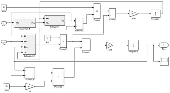
Figure 14.
Simulation model of a DTC system for a ship’s water cooling pump motor.
4. Results and Analysis of the Simulation
4.1. Results of the Simulation of the Stator’s Magnetic Chain in the Motor
The simulation parameters were as follows: amplitude of the stator’s chain, 1 Wb; width of the chain’s hysteresis loop, 0.01 Wb; width of the torque’s hysteresis loop, 1 N·m. The results of the simulation of the chain of the motor’s stator are shown in Figure 15 and Figure 16.
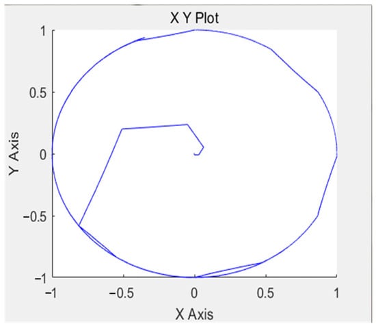
Figure 15.
Simulation results for the trajectory of the magnetic chain in the 6-ector model.

Figure 16.
Simulation results for the trajectory of the magnetic chain in the 12-sector model.
Direct torque control (DTC) was used to limit the errors in torque and the stator’s flux within the width of hysteresis by selecting an appropriate voltage vector for the stator. However, due to the switching between different voltage vectors with a discrete distribution, the flux changed abruptly, resulting in a rapid increase or decrease in the amplitude of flux, causing flux distortions and torque ripples. As can be seen from Figure 15, the trajectory of the stator chain in the 6-sector model started from a round point and gradually approached a circular trajectory in approximately 10 trajectory changes. By dividing the conventional six sectors of the stator’s flux into 12 sectors, more vectors could be selected without changing the circuit topology of the source inverter, and the torque ripple caused by alternating voltage vectors could be reduced, making the generated flux smoother. The trajectory of the stator’s chain under direct torque control in the 12-sector model shown in Figure 16 had a shorter excitation time than the 6-sector model, the waveform changed more gently, and the overall trajectory tended to be more circular. Therefore, after the analysis of the simulation results, it can be concluded that the division of 12 sectors had a certain suppression effect on the generation of magnetic chain pulsations, which could achieve a good dynamic response for the control of the ship water cooling pump motor and add reliability to the control of the ship water cooling pump motor.
4.2. Simulation Results of the Ship’s Central Water Cooling System
From the actual data of a 59,990 DWT bulk carrier, it is known that the rated power of the ship’s main engine is 10,680 kW, the seawater flow rate is 500 m3/h, the freshwater flow rate is 605 m3/h, the seawater temperature is 30 °C, and the temperature of the freshwater at the outlet is designed to be 36 °C. The corresponding simulation curves were obtained by inputting these data into the established simulation model, and then the energy-saving effects of the system were calculated and analyzed.
- (1)
- Simulation results under the rated operating conditions of the main engine
The conditions of the simulation were as follows: main load, 100%; temperature of the seawater, 30 °C; simulation time, 120 s. The results are shown in Figure 17.
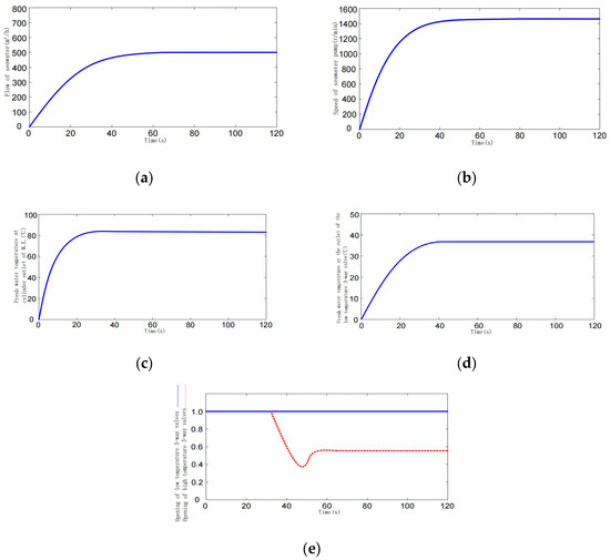
Figure 17.
(a–e) Results of the simulation under the rated operating conditions of the main engine. (a) Flow of seawater; (b) speed of the seawater pump; (c) temperature of the freshwater at the outlet of the cylinder of the ME; (d) temperature of the freshwater at the low-temperature three-way valve; (e) opening of the high- and low-temperature three-way valves.
Analysis of results. As can be seen in Figure 17, when the main engine was running at the rated power, the system reached a stable state at around 70 s, and the flow rate of the seawater was stable at 498 m3/h at this time, as can be seen in Figure 17a. The speed of the inverted seawater pump was 1445 r/min, as can be seen in Figure 17b, while the temperature of the freshwater at the outlet of the main engine’s cylinder sleeve was 84.4 °C (Figure 17c). The temperature of the freshwater at the outlet of the low-temperature three-way valve was maintained at around 35.8 °C, as seen in Figure 17d. From the simulation curve in Figure 17e, we can see that the degree of opening of the low temperature freshwater three-way valve was 100%. As can be seen from Table 1, when the simulated value was compared with the design value of the real ship, the error in the flow rate of seawater was 0.4% and the error in the speed of the seawater pump was 0.34%. The error values were within a reasonable range, so the results of this experimental model are more accurate and can be used as a reference for the real ship.

Table 1.
Comparison of errors in the main system’s parameters under the rated operating conditions.
- (2)
- Results of the simulation when the main power was reduced
The conditions of the simulation were as follows: the main load was reduced from 100% to 80%, the temperature of the seawater was 30 °C, and the simulation time was set to 120 s. The results are shown in Figure 18.

Figure 18.
(a–e) Results of the simulation when the main power was reduced. (a) Flow of seawater; (b) speed of the seawater pump; (c) temperature of the freshwater at the outlet of the cylinder of the M.E.; (d) temperature of the freshwater at the outlet of low-temperature three-way valve; (e) opening of the high- and low-temperature three-way valves.
As can be seen from the graph, the temperature of the seawater remained unchanged at 30 °C and the power of the main engine was reduced from 100% to 80%. At this time, the thermal load of each part of the cooling equipment in the central water cooling system was reduced, so the temperature of the cooling freshwater at the outlet of the low-temperature three-way valve was also reduced. In order to keep the temperature constant, the flow of seawater needed to be reduced, so the speed of the seawater pump was reduced. At the same time, in order to keep the freshwater temperature at the outlet of the main engine’s cylinder sleeve within a reasonable range, the opening of the high-temperature three-way valve needed to be increased to increase the flow of high-temperature freshwater. The system reached a stable state at around 100 s, and the flow rate of the seawater stabilized at 440 m3/h, as shown in Figure 18a. The speed of the inverted seawater pump was 1250 r/min, as shown in Figure 18b. The temperature of the freshwater at the outlet of the main cylinder sleeve was 83.1 °C, as shown in Figure 18c. The temperature of the freshwater at the outlet of the low-temperature three-way valve was maintained at around 36 °C, as seen in Figure 18d. The simulation curve in Figure 18e shows that the opening of the low-temperature three-way valve was 100%, and the opening of the high-temperature three-way valve was 78%.
- (3)
- Results of the simulation when the temperature of the seawater dropped
The conditions of the simulation were as follows: the main load was 100%, the temperature of the seawater dropped from 30 °C down to 18 °C, and the simulation time was set to 120 s. The results are shown in Figure 19.

Figure 19.
(a–e) Results of the simulation when the temperature of the seawater dropped. (a) Flow of seawater; (b) speed of the seawater pump; (c) temperature of the freshwater at the outlet cylinder of the M.E.; (d) temperature of the freshwater at the outlet of low-temperature three-way valve; (e) opening of the high- and low-temperature three-way valves.
As can be seen from the diagram, the main load was kept constant at 100% and the temperature of the seawater was lowered from 30 °C to 18 °C. As the temperature of the water cooling system decreased, the volume of the flow of seawater increased, so the flow of water for cooling can be reduced at this time by appropriately reducing the speed of the seawater pump. The decrease in the temperature of the seawater also caused the temperature of the freshwater at the outlet of the main engine’s cylinder sleeve to be lower than the set value, so the opening of the high-temperature three-way valve needed to be adjusted to further increase the flow of high-temperature freshwater. The system reached a stable state at around 90 s, and the flow rate of the seawater stabilized at 310 m3/h, as can be seen in Figure 19a. The speed of the inverted seawater pump was 940 r/min, as can be seen in Figure 19b, while the temperature of the freshwater at the outlet of the main cylinder sleeve was 83 °C, as seen in Figure 19c. The temperature of the freshwater at the outlet of the low-temperature three-way valve was maintained at around 36 °C, as shown in Figure 19d. The simulation curve in Figure 19e shows that the opening of the low-temperature freshwater three-way valve was 100%, and the opening of the high-temperature three-way valve was 59%.
- (4)
- Results of the simulation when the main engine’s power and the temperature of the seawater decreased simultaneously
The conditions of the simulation were as follows: the main load reduced from 100% to 80%, the temperature of the seawater was reduced from 30 °C to 18 °C, and the simulation time was set to 120 s. The results are shown in Figure 20.

Figure 20.
(a–e) Results of the simulation of a simultaneous drop in the main power and the temperature of the seawater. (a) Flow of seawater; (b) speed of the seawater pump; (c) temperature of the freshwater at the outlet cylinder of the M.E.; (d) temperature of the freshwater at the outlet of low temperature three-way valve; (e) opening of the high- and low-temperature three-way valves.
As can be seen from the graph, by reducing the main load from 100% to 80% and the temperature of the seawater from 30 °C to 18 °C, the temperature of the freshwater at the outlet of the low-temperature three-way valve was reduced significantly in a short period of time due to the reduction in the thermal load of each part of the cooling equipment and the reduction in the temperature in the water used for cooling. In order to cope with this change, the speed of the seawater pump needed to be reduced as soon as possible to reduce the flow of water for cooling. At the same time, the temperature of the freshwater at the outlet of the main engine’s cylinder liner also decreased due to the reduced heat load, so the opening of the high-temperature three-way valve needed to be increased to increase the flow of high-temperature freshwater, and thus increase the temperature of the main engine’s outlet. The system reached a stable state at around 105 s, and the flow rate of the seawater stabilized at 220 m3/h, as shown in Figure 20a. The speed of the inverted seawater pump was 710 r/min, as can be seen in Figure 20b. The temperature of the freshwater at the outlet of the main engine’s cylinder liner was 83 °C, as shown in Figure 20c. The temperature of the freshwater at the outlet of the low-temperature three-way valve was maintained at around 36 °C, as seen in Figure 20d. The simulation curve in Figure 20e shows that the opening of the low-temperature three-way valve was 45%, and the opening of the high-temperature three-way valve was 91%.
4.3. Results of the Simulation of the Motor’s Parameters
Table 2 shows the detailed parameters of the main seawater pump motor for the 59,990 DWT bulk carrier.
Table 2.
Detailed parameters of the main seawater pump motor for the 59,990 DWT bulk carrier.
- (1)
- Rated working conditions
Under the rated operating conditions, with a seawater inlet temperature of 30 °C and a diesel engine with 10,680 kW of power, the current, speed, and torque waveforms of the seawater pump motor for this system were as shown in Figure 21.
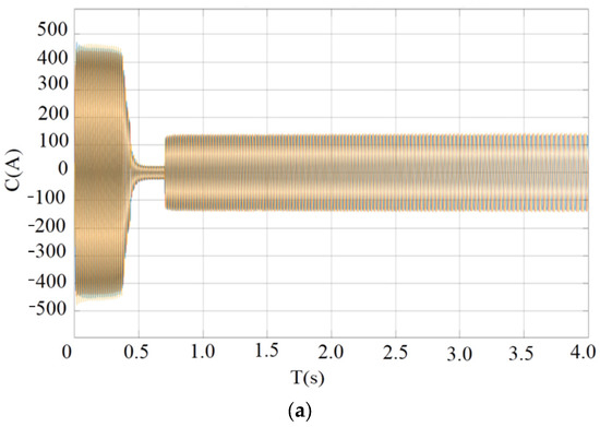
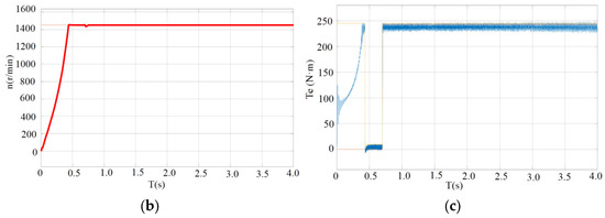
Figure 21.
(a–c) Parameters of the motor at the rated operating conditions. (a) Time vs. current; (b) time vs. speed; (c) time vs. torque.
When the main load was 100% and the temperature of the seawater was 30 °C, the results in Figure 21a show that when the system first started to run, the instantaneous current of the motor was large (about 450 A). The speed of the motor rose rapidly, as seen in Figure 21b. The electromagnetic torque (Figure 21c) rose instantaneously from 0 N·m to around 245 N·m, and the system reached a steady state at about 0.7 s. At this point, the current of the water cooling pump motor was about 130 A, the speed was about 1445 r/min, and the torque remained at about 243 N·m.
- (2)
- Results of the simulation when the main power was reduced
The conditions of the simulation were as follows: the main load was reduced from 100% to 80%, the temperature of the seawater was 30 °C, and the simulation time was set to 4 s. The results are shown in Figure 22.
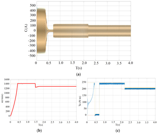
Figure 22.
(a–c) Parameters of the motor at reduced power. (a) Time vs. current; (b) time vs. speed; (c) time vs. torque.
For the simulation where the load of the main engine was reduced from 100% to 80%, and the temperature of the seawater was 30 °C, the results in Figure 22a show that when the load of the main engine changed abruptly, the current of the motor started to drop slowly and gradually, from 130 A to about 110 A, and the trend of the drop in current was relatively smooth. From Figure 22b, we can see that the speed of the motor also started to decrease accordingly from 1445 r/min to 1330 r/min. The electromagnetic torque (Figure 22c) decreased from 243 N·m to around 205 N·m. During the whole process of change, the dynamic response of the motor was fast and the change in torque was relatively smooth, and its fluctuation was also within a reasonable range. From the simulation curve, we can conclude that the system could have a good dynamic response when the main load changes abruptly, which means that the seawater pump motor can guarantee a fast response and achieve a dynamic balance at the same time.
- (3)
- Results of the simulation when the seawater temperature dropped
The conditions of the simulation were as follows: the main load was 100%, the temperature of the seawater dropped from 30 °C to 18 °C, and the simulation time was set to 4 s. The results are shown in Figure 23.
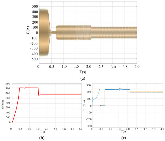
Figure 23.
(a–c) Parameters of the motor with a drop in seawater temperature. (a) Time vs. current; (b) time vs. speed; (c) time vs. torque.
For the simulation where the main load was 100% and the temperature of the seawater dropped from 30 °C to 18 °C, as can be seen from the results in Figure 23a, when the temperature of the seawater dropped, the current of the motor started to drop slowly and gradually, from 130 A to about 100 A. The trend of the drop in current was also relatively gentle. From Figure 23b, it can be seen that the motor’s speed also began to reduce from 1445 r/min. The electromagnetic torque (Figure 23c) was reduced from 243 N·m to around 195 N·m. Compared with the results for the rated operating conditions, the control system lowered the motor’s operating parameters effectively, the whole adjustment process was relatively smooth, and the system operated stably. The simulation curve showed that the system had a good dynamic response when the seawater temperature changed, and that the seawater pump motor could achieve good energy-saving effects.
- (4)
- Results of the simulation when the main power and the temperature of the seawater reduced at the same time
The conditions of the simulation were as follows: the main load was reduced from 100% to 80%, the temperature of the seawater was reduced from 30 °C to 18 °C, and the simulation time was set to 4 s. The results are shown in Figure 24.
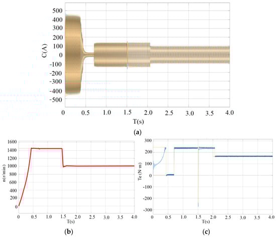
Figure 24.
(a–c) Parameters of the motor parameters for a simultaneous reduction in the main engine’s power and the temperature of the seawater. (a) Time vs. current; (b) time vs. speed; (c) time vs. torque.
When the load of the main engine was reduced from 100% to 80% and the temperature of the seawater was reduced from 30 °C to 18 °C, the results in Figure 24a showed that the current of the pump motor slowly decreased from 130 A to about 95 A, and the decrease in current was greater when compared with the first two working conditions, but the overall decreasing trend was still relatively gentle. The speed of the motor also decreased slowly from 1445 r/min to 1015 r/min, and the electromagnetic torque decreased from 243 N·m to around 164 N·m, as seen in Figure 24c. The simulation curve shows that the system had a good dynamic response in the face of simultaneous changes in the main load and the temperature of the seawater, the system maintained stable operations, and the energy-saving effects of the seawater pump were obvious.
5. Conclusions
By reviewing the data of the 59,990 DWT bulk carrier, we found that the average sailing time of the vessel was 5500 h throughout the year, from which the energy-saving effect of the inverter control system can be calculated.
- (1)
- Energy savings when the main engine’s load is reduced
When the load on the main machine was reduced from 100% to 80%, the power of the water cooling pump’s motor was 28.6 kW. The motor’s power was reduced from 37 kW to 28.6 kW, and the corresponding annual electrical energy consumption was reduced from 4.07 × 10⁵ kW·h to 3.146 × 10⁵ kW·h, which is a saving of approximately 22.70%.
- (2)
- Energy savings when the temperature of the seawater decreases
When the temperature of the seawater dropped from 30 °C to 18 °C, the power of the water cooling pump’s motor was 23.4 kW. The motor’s power was reduced from 37 kW to 23.4 kW, and the corresponding annual electrical energy consumption was reduced from 4.07 × 10⁵ kW·h to 2.574 × 10⁵ kW·h, a saving of approximately 36.76%.
- (3)
- Energy savings when the main engine’s load and the temperature of the seawater were reduced at the same time
When the main engine’s load was reduced from 100% to 80% and the temperature of the seawater was reduced from 30 °C to 18 °C, the power of the water cooling pump’s motor was 17.5 kW. The motor’s power was reduced from 37 kW to 17.5 kW, and the corresponding annual electricity consumption was reduced from 4.07 × 10⁵ kW·h to 1.925 × 10⁵ kW·h, a saving of approximately 52.70%.
Energy saving is becoming more and more important in today’s industry. These experimental results showed that the inverted control system had a better dynamic response and a more obvious energy-saving effect compared with the traditional industrial frequency system. When the frequency conversion control scheme described in this study was adopted, the marine cooling pump motor could save about 22.70%, 36.76%, and 52.70% of the electric energy throughout the year, thereby reducing the energy consumption of the entire ship. These values are for the energy saved within only one year, and the normal life of a ship is about 25 years, which means that a large amount of the energy consumption costs could be saved, providing some insights into the conservation of energy and a reduction in the emissions of ships. Research into the frequency conversion control system of the main seawater pump motor of the central water cooling system of a 59,990 DWT bulk carrier and the development of software to visualize the simulation can provide some reference for future research into the energy savings of the central water cooling systems of ships In this study, six sectors were divided into 12 sectors, but there were still some shortcomings. Although the fifth and seventh harmonic components weakened, the flux trajectory of the eleventh and thirteenth harmonic components increased compared with the model with six sectors. The division of the sectors could be further improved in subsequent studies.
Author Contributions
Writing—original draft, F.Z., L.S. and N.C.; Writing—review & editing, J.W. and Y.H. All authors have read and agreed to the published version of the manuscript.
Funding
This research received no external funding.
Data Availability Statement
The data presented in this study are available on request from the corresponding author. The data are not publicly available due to restrictions privacy or ethical.
Conflicts of Interest
The authors declare no conflict of interest.
References
- Osman, T. Energy efficient ship design and operations. Ocean. Eng. 2015, 110, 1. [Google Scholar]
- Dong, Y. Study on Low Carbon and Green Development of Tianjin Port Container Terminal. Master’s Thesis, Dalian Maritime University, Dalian, China, 2020. [Google Scholar]
- Lee, C.M.; Jeon, T.Y.; Jung, B.G.; Lee, Y.C. Design of Energy Saving Controllers for Central Cooling Water Systems. J. Mar. Sci. Eng. 2021, 9, 513. [Google Scholar] [CrossRef]
- Kocak, G.; Durmusoglu, Y. Energy efficiency analysis of a ship’s central cooling system using variable speed pump. J. Mar. Eng. Technol. 2018, 17, 43–51. [Google Scholar] [CrossRef]
- Dere, C.; Deniz, C. Load optimization of central cooling system pumps of a container ship for the slow steaming conditions to enhance the energy efficiency. J. Clean. Prod. 2019, 222, 206–617. [Google Scholar] [CrossRef]
- Zhang, R.-L.; Zhong, Z.-J.; Wang, Y.-X. Optimal control strategy for central cooling water system of ships. J. Guangzhou Marit. Acad. 2019, 27, 34–37. [Google Scholar]
- Kulkarni, C.; Hombal, G.; Angadi, S.; Raju, A.B. Direct Torque Control for Induction Motor Drive with Reduced Torque and Flux Ripples. Int. J. Recent Technol. Eng. 2020, 8, 101–106. [Google Scholar]
- Mahdi, J.; Karim, A.; Mustafa, M. A 12-sector space vector switching table for parallel-connecting to dual induction motors fed by matrix convertor based on direct torque control. SN Appl. Sci. 2021, 3, 849. [Google Scholar]
- Li, B. Research on Frequency Control of Marine Main Seawater Pumps and Energy Saving of the System. Master’s Thesis, Dalian Maritime University, Dalian, China, 2016. [Google Scholar]
- Gao, X. Optimization of Direct Torque Control Strategy for Asynchronous Motor without Speed Sensor. Master’s Thesis, Harbin Engineering University, Harbin, China, 2021. [Google Scholar]
- Alessandro, B.; Gianmarco, M.; Mario, M.; Massimiliano, P.; Luis, V. Induction Motor Direct Torque Control with Synchronous PWM. Energies 2021, 14, 5025. [Google Scholar] [CrossRef]
Disclaimer/Publisher’s Note: The statements, opinions and data contained in all publications are solely those of the individual author(s) and contributor(s) and not of MDPI and/or the editor(s). MDPI and/or the editor(s) disclaim responsibility for any injury to people or property resulting from any ideas, methods, instructions or products referred to in the content. |
© 2023 by the authors. Licensee MDPI, Basel, Switzerland. This article is an open access article distributed under the terms and conditions of the Creative Commons Attribution (CC BY) license (https://creativecommons.org/licenses/by/4.0/).