Abstract
Orthonormal subspace analysis (OSA) is proposed for handling the subspace decomposition issue and the principal component selection issue in traditional key performance indicator (KPI)-related process monitoring methods such as partial least squares (PLS) and canonical correlation analysis (CCA). However, it is not appropriate to apply the static OSA algorithm to a dynamic process since OSA pays no attention to the auto-correlation relationships in variables. Therefore, a novel dynamic OSA (DOSA) algorithm is proposed to capture the auto-correlative behavior of process variables on the basis of monitoring KPIs accurately. This study also discusses whether it is necessary to expand the dimension of both the process variables matrix and the KPI matrix in DOSA. The test results in a mathematical model and the Tennessee Eastman (TE) process show that DOSA can address the dynamic issue and retain the advantages of OSA.
1. Introduction
Process monitoring and fault detection are two important aspects of process systems engineering because they are the key issues to address in order to ensure the safety and the normal operation of industrial processes [1].As such, traditional data-driven algorithms such as principal components analysis (PCA) [2] and independent components analysis (ICA) [3] have been proposed to monitor processes and to improve the product quality. PCA and ICA can effectively detect faults in a process. However, in the actual production process at a modern industrial plant, there are a large number of controllers, sensors and actuators distributed widely, and not all data need to be analyzed [4,5]. That is to say, not all process variables directly affect the safety and the product quality. The information highly relevant to the product quality and economic benefits are called key performance indicators (KPIs), and their role should be emphasized in process monitoring [6,7]. It is worth mentioning that both PCA and ICA monitor KPI-related and KPI-unrelated components simultaneously, and they perform poorly in detecting faults in KPI-related components because the fault information might be submersed in the disturbances of numerous KPI-unrelated components. As such, KPI-related process monitoring such as partial least squares (PLS) [8] and canonical correlation analysis (CCA) [9] algorithms have developed rapidly in recent decades, and this development is essential for ensuring production safety and obtaining superior operation performance.
However, there are still some drawbacks to these traditional KPI algorithms. First, the residual subspace calculated by the PLS algorithm is non-orthogonal to the principal components (PCs) subspace, which means that some KPI-related information may leak into the residual spaces [10,11]. Second, the CCA algorithm requires KPIs to be available during both offline training and online monitoring stages as it uses KPI variables to construct indices [12,13]. Third, both PLS and CCA algorithms are unable to extract PCs [14,15].
To address the above issues in traditional KPI-related algorithms, Lou et al. proposed orthonormal subspace analysis (OSA) [16]. OSA can divide the process data and KPIs into three orthonormal subspaces, namely, subspaces of KPI-related components, KPI-unrelated components in process data, and process-unrelated components in KPIs. Furthermore, the cumulative percent variance method is used to select the number of PCs in an OSA algorithm. Due to the ability of the OSA algorithm to independently monitor each subspace, the OSA algorithm is not limited by KPIs during the offline and online stages.
The original OSA was proposed for addressing the monitoring issues in static process problems, so it assumes that the observations are time-independent. However, dynamic features widely exist in most industrial processes, and, hence, the auto-correlation relationships in variables interfere with the extraction of the KPI-related information [17,18]. Therefore, the subspaces obtained by the OSA algorithm are not orthonormal in dynamic processes.
The “time lag shift” method, which lists the historical data as additional variables to the original variable set, is an effective measure for handling the dynamic issue, and it has been adopted in the PLS and CCA algorithms, i.e., the dynamic PLS (DPLS) and dynamic CCA (DCCA) algorithms. Therefore, in this paper, the “time lag shift” method is also combined with the OSA algorithm, named the dynamic OSA (DOSA) algorithm, and is applied to the Tennessee Eastman (TE) process to illustrate its efficiency.
The contributions of this study are as follows. First, this study proposes DOSA for dealing with the low detection rate problem caused by the dynamics processes. DOSA can determine whether the fault in a dynamics process originates from KPI-related or KPI-unrelated process variables or the measurement of KPIs. Second, this study discusses whether it is necessary to expand the dimension of both the process variables matrix and the KPI matrix in order to reduce the computation. At the same time, a new method to select the time lag number in the “time lag shift” structure is proposed. Additionally, we analyze the impact of the sampling period on DOSA. Third, we place an emphasis on the real-time nature of information and design new monitoring indices. Finally, this study compares the detection rates of the OSA, DOSA, DPLS, and DCCA algorithms.
The remainder of this paper is organized into five sections. Section 2 discusses the classical OSA algorithm and the “time lag shift” method. Section 3 proposes DOSA for dynamics process monitoring. Section 4 compares the DOSA algorithm with other KPI-related algorithms based on TE process testing. Section 5 reviews the contributions of this work.
2. Methods
2.1. Orthonormal Subspace Analysis
Here, we take as the process variables matrix (where is the number of samples, and is the number of process variables), and the standard PLS identification technique introduces the KPI matrix as (where is the number of KPIs). OSA decomposes both and into the following bilinear terms:
where ( is the number of principal components) is the common latent variables shared by and ; and are the transformation matrices; and and are the residual matrices.
Then, OSA, along with PLS and CCA, is called ‘KPI-related algorithm’. As opposed to PLS and CCA, the extracted subspaces of OSA are proved to be orthogonal [16]. That is to say, , , and are orthogonal in Equation (1), and, most importantly, they can be monitored independently.
2.2. The “Time Lag Shift” Method
The proposed OSA algorithm in Section 2.1 implicitly assumes that the current observations are statistically independent to the historical observations [19,20]. That is to say, OSA only considers the correlation between variables at the same time but does not consider the mutual influence of variables at different times. However, most data from industrial processes show degrees of dynamic characteristics; that is, the sampling data at different times are correlated. For such a process, the static OSA algorithm is not applicable.
The most common method to address such a problem is to use an autoregressive (AR) model to describe the dynamic characteristics. Similarly, the OSA algorithm can be extended to take into account the serial correlations by augmenting each observation vector, or , at the current time with the previous or observations in the following manner [21]:
As known in Equation (2), the first columns of and the first columns of represent the data at the current time, and the rest represent the data at the past time. For sampling times, one can obtain the augmented matrices and .
By performing dimension expansion on the data matrix in Equation (2), the static OSA methods can be used to analyze the autocorrelation, cross-correlation, and hysteresis correlation among the data synchronously. That is to say, and will be decomposed by OSA. More details can be found in Section 3.
3. Dynamics Orthonormal Subspace Analysis
3.1. Determination of the Lag Number
As the traditional lag determination methods, such as the Akaike information criterion (AIC) [22] and the Bayesian information criterion (BIC) [23], are only suitable for a steady state, a new lag determination method should be proposed for DOSA.
Suppose the relationship between the data at the current time and the past time is as follows:
where ,, , and . and denote the disturbance introduced at each time, and it is statistically independent of the past data. The coefficient matrices and can be estimated from the least square method as follows:
Therefore, and can be estimated as follows:
Then, the optimal number of time lag will be the one that creates the following indices:
the minimum and the indices will not change significantly if we continue increasing the time lag.
As opposed to and , and are time-uncorrelated and independent of the initial states of and , so they can be adopted to the dynamic process in both steady and unsteady states.
Additionally, we also set up an index to describe ‘the value of Lagx or Lagy would not change significantly’ as shown in Equation (7):
where represents the value of or when the lag number is or , and represents the value of Lagx or Lagy when the lag number is or . If the value of begins to be less than 5%, we will say that ‘the value of or would not change significantly’.
3.2. DOSA Procedure
- Step 1. The “Time Lag Shift” method mentioned in Section 2.2. Calculate the lag number of and in Equation (6). Then, augment and with the previous observations shown in Equation (2). In doing so, we can obtain the augmented matrix and with n samples.
- Step 2. Traditional OSA mentioned in Section 2.1.
- (a)
- Calculate the Y-related component and the X-related component using Equation (8). and are both called ‘the common component’ and are shown to be equal in reference [16], as shown below:
We tend to focus on process variables related to KPIs in industrial processes. By extracting common components and monitoring them (Step 3), one can know whether there are faults in the variables related to KPIs.
- (b)
- Calculate the non-Y-related component and the non-X-related component aswhere EOSA and FOSA are both called ‘the unique component’. By extracting and monitoring the unique components (Step 3), one can know whether there are faults in the variables unrelated to KPIs.
- (c)
- Extract the PCs in XOSA using the PCA decomposition method because the variables in XOSA might be highly correlated:where represents the score matrix of the common component; is the loading matrix of the common component; is the residual matrix; and k is the number of PCs. In this step, the PCs are selected by using the CPV method, and the threshold value follows the PCA criterion, e.g., 85%.
In theory, the score matrices of the common components and are equal unless there is something wrong with the relationship between X and Y. We use the sum of squares of the score matrices to monitor whether there are faults in the relationship between X and Y (Step 3). Similarly to Equation (10), the score matrix of the common component is .
- Step 3. Monitoring indices calculation.
Taking into account the real-time nature of the information, PCA monitoring is not directly performed for , EOSA, and because these components contain a great amount of information at the past time. The calculation of the indices if as follows:
- (a)
- The first columns of XOSA are monitored by the PCA approach and can then be used to generate the and indices. That is to say, we only monitor the data at the current time.
- (b)
- Similarly, the first columns of and the first columns of can be monitored by the PCA approach and can then be used to generate the indices , , , and .
- (c)
- Furthermore, if there is something wrong with the relationship between X and Y, there will be significant differences between the score matrices and . Therefore, the following index can be used to test the abnormal relationship:
Figure 1 summarizes the procedure presented below.
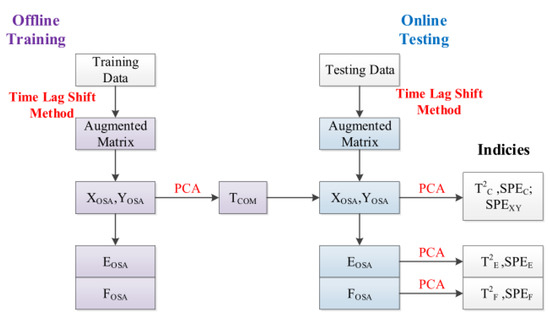
Figure 1.
The flow chart of DOSA.
3.3. A Dynamics Model Analyzed with DOSA
3.3.1. Dynamics Model
To analyze the characteristics of the DOSA method and compare its performance with the OSA algorithm, we use a simplistic simulation process in illustrating the monitoring performances of them. Consider a large-scale process in which each single subprocess can be expressed using a time-invariant, state-space model as follows:
where , , and are independent Gaussian distributed vectors; and are the noisy components, which are independent of the process measurements; and C and E and D and F are the coefficient matrices of the dynamic and static parts, respectively. Here, we take three algorithms into consideration: OSA; the DOSA that expands the dimension of , which is denoted as DOSA-X; the DOSA that expands the dimension of both and , which is denoted as DOSA-XY.
3.3.2. The Optimal Numbers of Time Lag
To determine the number of time lag, the dynamics model with several numbers of lags that are different from the normal data are fitted. Here, and are the numbers of lags in matrix X and Y, respectively. In this work, we set and , and several values of and are shown in Figure 2 and Figure 3.
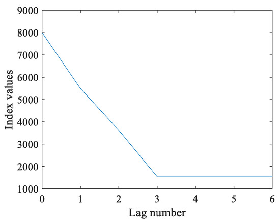
Figure 2.
The values of under different values.
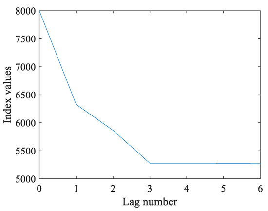
Figure 3.
The values of under different values.
From the analyses shown in Figure 2 and Figure 3, the values of would be lowest if was less than or equal to 3, and the values of tended to be lowest if was less than or equal to 3. At this time, the values of both and would not decrease significantly if we continued increasing the values of and . Therefore, the optimal lag numbers were and , and this can be seen intuitively in the diagram. Furthermore, the several values of , , and are listed in Table 1 and Table 2.

Table 1.
The values of under different values.
Table 2.
The values of under different values.
From the data presented in Table 1 and Table 2, the values of were less than 5% when lx and ly gradually increased from 3. This also means that the optimal numbers of lags were lx = 3 and ly = 3, which is consistent with the true value.
Here, we take the traditional BIC method, which has a larger penalty than the AIC, as an example to calculate the optimal number of this model. When selecting the best model from a set of alternative models, the model with the lowest BIC should be chosen.
From the data presented in Table 3 and Table 4, the optimal numbers of lags were and . However, we introduced a third-order lag as Section 3.3.1 mentioned. Therefore, instead of the BIC, the original method of this work was applied to test the algorithm.
Table 3.
The values of BIC under different values.
Table 4.
The values of BIC under different values.
3.3.3. Testing Results
(a) Fault 1: a step change with an amplitude of 3 in . Certainly, the static parameter is the unique part of . The detection rates and false alarm rates of three algorithms are shown in Table 5. In Table 5, the detection rate of was extremely high, so we could correctly infer that the fault occurred in the unique part of . In other words, it is possible that there was a fault in the process variables instead of in the measurement of the KPIs. It is more important that the detection rates of the two dynamics monitoring methods were higher than the detection rate of the OSA. Thus, the dynamics problem could be solved by DOSA in this case. Furthermore, the effect of the dimension expansion for both and was better than the dimension expansion for alone. It can be hypothesized that expanding the dimension of the matrix can improve the sensitivity of the algorithm to the fault.
Table 5.
Fault 1 detection rates and false alarm rates of three algorithms.
(b) Fault 2: a step change with an amplitude of 3 in . It is obvious that the static parameter is the unique part of . The results are shown in Table 6. As can be seen in Table 6, we had already expanded the dimension of , but the detection rates of all of the indices were extremely low. Then, we found that the index performed better while expanding the dimension of both and . This means that the fault occurred in the unique part of . That is to say, there was a fault in the measurement of the KPIs instead of the process variables. In addition, the detection rate of DOSA-XY was extremely higher than the other two algorithms. Thus, an algorithm for the dimension expansion of data matrices with dynamic processes performs well while also solving the dynamics issue.
Table 6.
Fault 2 detection rates and false alarm rates of three algorithms.
(c) Fault 3: a step change with an amplitude of 3 in . Certainly, the static parameter is the common part of both and . The results are shown in Table 7. As can be seen in Table 7, we could not judge the location of the fault if we did not expand the dimension of Y because the detection rates of most of the indices were about 50%. Then, the index performed better while expanding the dimension of both and . This means that the fault occurred in the common part of both and . That is to say, there was a fault in both the process variables and in the measurement of the KPIs. In addition, the detection rate of DOSA-XY was extremely higher than that of the other two algorithms. Thus, an algorithm for the dimension expansion of data matrices with dynamic processes performs well while dealing with the dynamics issue.
Table 7.
Fault 3 detection rates and false alarm rates of three algorithms.
(d) Fault 4: the matrix changed to :
Generally, the coefficient matrix affects the relationship of and . The results are shown in Table 8. In Table 8, the index SPEXY that specifically detects the relationship of and performed well. We could infer that there was a high probability of a fault in or . Then, the detection rate of DOSA-XY was extremely higher than that of the other two algorithms. Thus, an algorithm for the dimension expansion of both and performs well while also solving the dynamics issue.
Table 8.
Fault 4 detection rates and false alarm rates of three algorithms.
3.3.4. The Influence of Sampling Period on DOSA
In sum, it is necessary to expand the dimension of both and . In this section, we will take the effect of the sampling rate on the DOSA algorithm into account. The dynamics models and faults in Section 3.3.1 and Section 3.3.3 still apply to this section.
Firstly, the section will discuss the effect of doubling the sampling period on the selection of the lag number. We still set and , followed by several values of and , and the corresponding changes in rate are listed in Table 9 and Table 10.
Table 9.
The values of for doubling the sampling period.
Table 10.
The values of for doubling the sampling period.
As shown in Table 9 and Table 10, the optimal lag numbers were and because the values of were less than 5% when and gradually increased from 1. That is to say, the optimal lag numbers were affected by the sampling period. Thus, the effect of the sampling period on the detection rates of the DOSA was also a concern.
- (a)
- Fault 1: the fault occurs in the unique part of . The experimental comparison of the primitive and doubled sampling periods is shown in Table 11. As also shown in the table, the detection rate of decreased by about 9%, and the detection rate of decreased by about 4%.
Table 11. Comparison of primitive and doubled sampling periods (Fault 1).
- (b)
- Fault 2: the fault occurs in the unique part of . The experimental comparison of the primitive and doubled sampling periods is shown in Table 12. As also shown in the table, the detection rate of decreased by about 8%, and the detection rate of decreased by about 3%.
Table 12. Comparison of primitive and doubled sampling periods (Fault 2).
- (c)
- Fault 3: the fault occurs in the common part of and . The experimental comparison of the primitive and doubled sampling periods is shown in Table 13. As also shown in the table, the detection rate of decreased by about 8%, and the detection rate of decreased by about 5%.
Table 13. Comparison of primitive and doubled sampling periods (Fault 3).
- (d)
- Fault 4: the fault occurs in the coefficient matrix , which affects the relationship of and . The experimental comparison of the primitive and doubled sampling periods is shown in Table 14. As can be seen in Table 14, there was no significant change in the detection rate of .
Table 14. Comparison of primitive and doubled sampling periods (Fault 4).
Based on the above testing results, we can see that the change in sampling period affected the determination of the lag numbers. The detection rates were also slightly affected. That is to say, the DOSA algorithm is sensitive to the change in sampling period because the AR model, which is constructed by the DOSA, will be different with the change in sampling period. We hope to solve this problem as we continue our improvement of this project in the future.
3.4. Conclusion
As shown by the above results, we can conclude the following:
- (1)
- It is necessary to expand the dimension of both and .
- (2)
- DOSA could adequately solve the dynamics issue.
- (3)
- DOSA is able to directly analyze the location of the fault. Thus, we can know whether a fault actually occurs in KPI-related process variables, KPI-unrelated process variables, and the measurement of the KPIs.
- (4)
- DOSA is sensitive to the change in sampling period.
4. Comparison Study Based on Tennessee Eastman Process
4.1. Tennessee Eastman Process
In this section, we would like to briefly introduce an industrial benchmark of the Tennessee Eastman (TE) process [24,25]. All the discussed methods will be further applied to demonstrate their efficiencies. The TE process model is a realistic simulation program of a chemical plant, which is widely accepted as a benchmark for control and monitoring studies [26]. The flow diagram of the process is described in [27,28], and the FORTRAN code of the process is available on the Internet. The process has two products from four reactants as shown in Equation (14):
The TE process has 52 variables, including 41 process variables and 11 manipulated variables. Table 15 lists a set of 15 known faults introduced to the TE process. Training and test sets have been collected by running 25 and 48 h simulations, respectively, in which faults have been introduced 1 and 8 h into the simulation, and each variable is sampled every 3 min. Thus, training sets consist of 500 samples, whereas test sets contain 960 samples per set of simulation [29,30].
Table 15.
Descriptions of known faults in TE process.
4.2. The Numbers of Time Lag in TE Process
Here, and are the lag numbers in the augmented process variables matrix and the augmented KPI matrix, respectively. In this work, we set and . Several values of Lagx and Lagy and their corresponding changes in rate are listed in Table 16 and Table 17.
Table 16.
The values of under different values.
Table 17.
The values of under different values.
From the data presented in Table 16 and Table 17, the values of tended to be the lowest, and the values of tended to be the lowest if was less than or equal to 3. At this time, the values of the rate of change were less than 5% when gradually increased from 3. That is to say, the values of would not decrease significantly if we continued increasing Ly. Therefore, the optimal numbers of lags were and .
4.3. Simulation Study
We tend to focus on the ability to detect KPI-related faults in the TE process. Table 18 lists a set of nine KPI-related faults introduced to the TE process. It shows the detection and false alarm rates for four algorithms: OSA, DOSA, Dynamics CCA (DCCA), and Dynamics PLS (DPLS).
Table 18.
Testing results of KPI-related faults for the TE process.
Considering the data presented in Table 18, DOSA shows better performance compared to the other algorithms for KPI-related faults. Meanwhile, the DOSA algorithm showed a great advantage in Faults 1–2, 8, and 12–13 over the OSA algorithm. From this analysis, it can be concluded that the DOSA algorithm performs better than the OSA algorithm on dynamic problems. Figure 4 shows the simulation diagram of OSA and DOSA monitoring in these faults. The blue line represents the value of the statistic, and the red line represents the value of the control limit. When the blue line is higher than the red line, a fault has occurred. It is obvious that the DOSA algorithm is more sensitive to these faults.
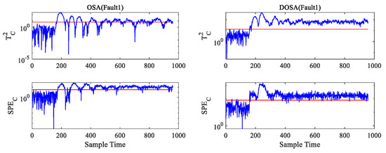
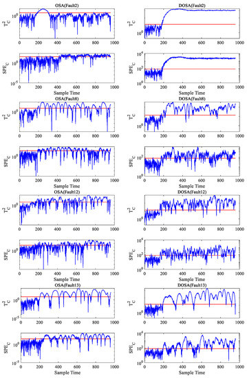
Figure 4.
The simulation comparison of OSA and DOSA monitoring in Faults 1–2, 8, and 12–13.
5. Conclusions
In this paper, we have presented an improved algorithm of OSA for conducting large-scale process monitoring, called the DOSA algorithm, and compared its performance against DPLS and DCCA, which are KPI-related algorithms that are also used to solve dynamic problems.
Considering the testing results of the dynamics model, this article proved that it is necessary to expand the dimension of both the process variables matrix and the KPI matrix while using the DOSA algorithm. Furthermore, the DOSA algorithm is able to adequately solve the dynamics issue; Thus, we can know whether a fault actually occurs in the KPI-related or KPI-unrelated process variables or in the measurement of the KPIs.
The comparative study was conducted using the Tennessee Eastman benchmark process, and we can conclude that the DOSA algorithm achieves better detection rates of faults from the analysis of the results obtained. However, the DOSA algorithm is sensitive to the change in sampling period. We intend to solve this problem as we continue the improvement of this project in the future.
Author Contributions
Conceptualization, W.H.; methodology, W.H. and Z.L.; validation, S.L.; formal analysis, W.H.; resources, Y.W. and S.L.; writing—original draft preparation, W.H.; writing—review and editing, Z.L. and W.H.; visualization, W.H.; supervision, S.L., X.J., and S.D.; project administration, Z.L.; funding acquisition, S.L. and Z.L. All authors have read and agreed to the published version of the manuscript.
Funding
This work was supported by the Natural Science Foundation of Guangdong Province, China (NO. 2022A1515011040), the Natural Science Foundation of Shenzhen, China (NO. 20220813001358001) and the Young Talents program offered by the Department of Education of Guangdong Province, China (2021KQNCX210).
Data Availability Statement
The data that support the findings of this study are available from the corresponding author upon reasonable request.
Conflicts of Interest
The authors declare no conflict of interest.
References
- Zhu, J.; Jiang, M.; Liu, Z. Fault Detection and Diagnosis in Industrial Processes with Variational Autoencoder: A Comprehensive Study. Sensors 2022, 22, 227. [Google Scholar] [CrossRef]
- Zhao, F.; Rekik, I.; Lee, S.W.; Liu, J.; Zhang, J.; Shen, D. Two-Phase Incremental Kernel PCA for Learning Massive or Online Datasets. Complexity 2019, 2019, 5937274. [Google Scholar] [CrossRef]
- Zhang, S.; Zhao, C. Hybrid Independent Component Analysis (H-ICA) with Simultaneous Analysis of High-Order and Second-Order Statistics for Industrial Process Monitoring. Chemom. Intell. Lab. Syst. 2019, 185, 47–58. [Google Scholar] [CrossRef]
- Qin, Y.; Lou, Z.; Wang, Y.; Lu, S.; Sun, P. An Analytical Partial Least Squares Method for Process Monitoring. Control. Eng. Pract. 2022, 124, 105182. [Google Scholar] [CrossRef]
- Yin, S.; Zhu, X.; Kaynak, O. Improved PLS Focused on Key-Performance-Indicator-Related Fault Diagnosis. IEEE Trans. Ind. Electron. 2015, 62, 1651–1658. [Google Scholar] [CrossRef]
- Wang, H.; Gu, J.; Wang, S.; Saporta, G. Spatial Partial Least Squares Autoregression: Algorithm and Applications. Chemom. Intell. Lab. Syst. 2019, 184, 123–131. [Google Scholar] [CrossRef]
- Tao, Y.; Shi, H.; Song, B.; Tan, S. Parallel Quality-Related Dynamic Principal Component Regression Method for Chemical Process Monitoring. J. Process Control 2019, 73, 33–45. [Google Scholar] [CrossRef]
- Sim, S.F.; Jeffrey Kimura, A.L. Partial Least Squares (PLS) Integrated Fourier Transform Infrared (FTIR) Approach for Prediction of Moisture in Transformer Oil and Lubricating Oil. J. Spectrosc. 2019, 2019, e5916506. [Google Scholar] [CrossRef]
- Kanatsoulis, C.I.; Fu, X.; Sidiropoulos, N.D.; Hong, M. Structured SUMCOR Multiview Canonical Correlation Analysis for Large-Scale Data. IEEE Trans. Signal Process. 2019, 67, 306–319. [Google Scholar] [CrossRef]
- Cai, J.; Dan, W.; Zhang, X. ℓ0-Based Sparse Canonical Correlation Analysis with Application to Cross-Language Document Retrieval. Neurocomputing 2019, 329, 32–45. [Google Scholar] [CrossRef]
- Su, C.H.; Cheng, T.W. A Sustainability Innovation Experiential Learning Model for Virtual Reality Chemistry Laboratory: An Empirical Study with PLS-SEM and IPMA. Sustainability 2019, 11, 1027. [Google Scholar] [CrossRef]
- Alvarez, A.; Boente, G.; Kudraszow, N. Robust Sieve Estimators for Functional Canonical Correlation Analysis. J. Multivar. Anal. 2019, 170, 46–62. [Google Scholar] [CrossRef]
- de Cheveigné, A.; Di Liberto, G.M.; Arzounian, D.; Wong, D.D.E.; Hjortkjær, J.; Fuglsang, S.; Parra, L.C. Multiway Canonical Correlation Analysis of Brain Data. NeuroImage 2019, 186, 728–740. [Google Scholar] [CrossRef]
- Tong, C.; Lan, T.; Yu, H.; Peng, X. Distributed Partial Least Squares Based Residual Generation for Statistical Process Monitoring. J. Process Control 2019, 75, 77–85. [Google Scholar] [CrossRef]
- Si, Y.; Wang, Y.; Zhou, D. Key-Performance-Indicator-Related Process Monitoring Based on Improved Kernel Partial Least Squares. IEEE Trans. Ind. Electron. 2021, 68, 2626–2636. [Google Scholar] [CrossRef]
- Lou, Z.; Wang, Y.; Si, Y.; Lu, S. A Novel Multivariate Statistical Process Monitoring Algorithm: Orthonormal Subspace Analysis. Automatica 2022, 138, 110148. [Google Scholar] [CrossRef]
- Song, Y.; Liu, J.; Chu, N.; Wu, P.; Wu, D. A Novel Demodulation Method for Rotating Machinery Based on Time-Frequency Analysis and Principal Component Analysis. J. Sound Vib. 2019, 442, 645–656. [Google Scholar] [CrossRef]
- Zhang, C.; Guo, Q.; Li, Y. Fault Detection Method Based on Principal Component Difference Associated with DPCA. J. Chemom. 2019, 33, e3082. [Google Scholar] [CrossRef]
- Dong, Y.; Qin, S.J. A Novel Dynamic PCA Algorithm for Dynamic Data Modeling and Process Monitoring. J. Process Control 2018, 67, 1–11. [Google Scholar] [CrossRef]
- Oyama, D.; Kawai, J.; Kawabata, M.; Adachi, Y. Reduction of Magnetic Noise Originating from a Cryocooler of a Magnetoencephalography System Using Mobile Reference Sensors. IEEE Trans. Appl. Supercond. 2022, 32, 1–5. [Google Scholar] [CrossRef]
- Lou, Z.; Shen, D.; Wang, Y. Two-step Principal Component Analysis for Dynamic Processes Monitoring. Can. J. Chem. Eng. 2018, 96, 160–170. [Google Scholar] [CrossRef]
- Sakamoto, W. Bias-reduced Marginal Akaike Information Criteria Based on a Monte Carlo Method for Linear Mixed-effects Models. Scand. J. Stat. 2019, 46, 87–115. [Google Scholar] [CrossRef]
- Gu, J.; Fu, F.; Zhou, Q. Penalized Estimation of Directed Acyclic Graphs from Discrete Data. Stat. Comput. 2019, 29, 161–176. [Google Scholar] [CrossRef]
- Wan, J.; Li, S. Modeling and Application of Industrial Process Fault Detection Based on Pruning Vine Copula. Chemom. Intell. Lab. Syst. 2019, 184, 1–13. [Google Scholar] [CrossRef]
- Huang, J.; Ersoy, O.K.; Yan, X. Fault Detection in Dynamic Plant-Wide Process by Multi-Block Slow Feature Analysis and Support Vector Data Description. ISA Trans. 2019, 85, 119–128. [Google Scholar] [CrossRef]
- Plakias, S.; Boutalis, Y.S. Exploiting the Generative Adversarial Framework for One-Class Multi-Dimensional Fault Detection. Neurocomputing 2019, 332, 396–405. [Google Scholar] [CrossRef]
- Zhao, H.; Lai, Z. Neighborhood Preserving Neural Network for Fault Detection. Neural Netw. 2019, 109, 6–18. [Google Scholar] [CrossRef]
- Suresh, R.; Sivaram, A.; Venkatasubramanian, V. A Hierarchical Approach for Causal Modeling of Process Systems. Comput. Chem. Eng. 2019, 123, 170–183. [Google Scholar] [CrossRef]
- Amin, M.T.; Khan, F.; Imtiaz, S. Fault Detection and Pathway Analysis Using a Dynamic Bayesian Network. Chem. Eng. Sci. 2019, 195, 777–790. [Google Scholar] [CrossRef]
- Cui, P.; Zhan, C.; Yang, Y. Improved Nonlinear Process Monitoring Based on Ensemble KPCA with Local Structure Analysis. Chem. Eng. Res. Des. 2019, 142, 355–368. [Google Scholar] [CrossRef]
Disclaimer/Publisher’s Note: The statements, opinions and data contained in all publications are solely those of the individual author(s) and contributor(s) and not of MDPI and/or the editor(s). MDPI and/or the editor(s) disclaim responsibility for any injury to people or property resulting from any ideas, methods, instructions or products referred to in the content. |
© 2023 by the authors. Licensee MDPI, Basel, Switzerland. This article is an open access article distributed under the terms and conditions of the Creative Commons Attribution (CC BY) license (https://creativecommons.org/licenses/by/4.0/).