Article

CFD Simulation on Pressure Profile for Direct Contact Condensation of Steam Jet in a Narrow Pipe

1
School of Thermal Engineering, Shandong Jianzhu University, Jinan 250101, China
2
Shandong Lurun Heat Energy Science & Technology Co., Ltd., Jinan 250305, China
3
School of Energy and Power Engineering, Shandong University, Jinan 250061, China
4
Northwest Institute of Nuclear Technology, Xi’an 710024, China
5
Science and Technology on Thermal Energy and Power Laboratory, Wuhan Second Ship Design and Resource Institute, Wuhan 430205, China
6
School of New Energy, Xi’an Shiyou University, Xi’an 710065, China
*
Authors to whom correspondence should be addressed.
Processes 2023, 11(6), 1821; https://doi.org/10.3390/pr11061821
Submission received: 4 May 2023 / Revised: 2 June 2023 / Accepted: 13 June 2023 / Published: 15 June 2023

Abstract

:
In the published experimental results, it has been observed that when high-speed steam spurt into the subcooled waterflow, the total pressure along the axial direction at trailing edge of the steam plume shows a pressure-lift. To reveal the mechanism behind this phenomenon, this study utilizes a particle model to investigate the pressure profile of steam jet condensation in subcooled water flow in a narrow pipe. A numerical model based on the Eulerian–Eulerian multiphase model has been developed to accurately simulate the characteristics of pressure profile along the axial direction. The model’s validity is established by comparing the steam plume shape and temperature profiles with the experimental data. By analyzing the total pressure profile of the axis and the contours of gas volume fraction, it is found that there exists a pressure-lift phenomenon at trailing edge of the steam plume. The dynamic pressure of the water also shows a pressure-lift at this position, so it can be inferred that the dynamic pressure of the water is the main factor of the total pressure-lift.

1. Introduction

Due to the efficient heat and mass transfer, direct contact condensation (DCC) of a submerged steam jet in a narrow pipe is widely employed in all kinds of industrial occasions, such as nuclear power plants, direct contact condensers [1,2,3], district heating equipment, steam injectors, and refrigeration systems.
In the field of interphase mass transfer in for DCC, various models have been proposed by researchers to understand and optimize the complex physical processes involved [4]. The present study provides an overview of some of the relevant literature on numerical modeling of DCCs with a focus on steam jet condensation. Gulawani et al. [5] proposed a thermal phase change model to solve the interphase heat and mass transfer for steam jet in quiescent water. The model is applicable only for phase change phenomenon in pure substances. Shah et al. [6,7] proposed a Eulerian–Eulerian two-phase flow model combined with the realizable k-ε turbulence model to study the heat transfer and flow characteristics of a steam jet pump. They employed Fluent 6.3 to analyze the steam jet pump. Zhou [8,9] observed four types of steam plume shapes by numerical analysis, and the internal flow mechanism was explained by the theory of compression and expansion waves, respectively. Qu et al. [10,11,12] simulated the steam–air jet and found that the non-condensable air will deteriorate the DCC process based on the gas void fractions and the axial temperature profile. Patel [13] carried out the numerical simulations of DCC phenomenon in a suppression pool combined with two kinds of commercial CFD software. To investigate chugging flow during DCC in Boiling Water Reactor (BWR) suppression pools, Tanskanen [14] utilized numerical method with a two-dimensional method via the NEPTUNE_CFD software. Li [15] performed a numerical analysis for chugging flow using a Volume of Fluid (VOF) model and Large Eddy Simulation (LES) model. The model’s accuracy was validated with the experimental data conducted by Chan and Lee [16].
Some researchers have measured the flow field parameter during the stable steam jet process. In an experimental study on DCC of a stable steam discharging into the quiescent water by Kim [17], the axial and radial temperature profiles were examined, and they found that the ellipsoidal steam plume is due to the expansion and compression waves. Del Tin [18] measured the total pressure profiles inside the jet core region and the surrounding water. The total pressure along the jet axis was found to be higher than the inlet steam pressure. However, a detailed description could not be provided due to the complexity of the situation. Yan et al. [19] measured the axial total pressures for low mass flux steam jet in subcooled water, and found it decreases initially and then increases with the axial distance, reaching a peak before returning to ambient pressure. A dimensionless correlation for predicting the peak distance of total pressure is obtained. Moreover, the axial total pressure is significantly influenced by the subcooled water temperature, and the peak decreases as the water temperature increases until it disappears. Wu et al. [20,21] also measured the axial total pressures in the jet region under a wide range of operating conditions. Due to the condensation shock wave, the maximum pressure along the axis is even larger than the steam inlet pressure. The maximum lifting-pressure coefficient was calculated under the conditions of steam inlet pressure, water temperature, and pressure ratio. However, the reason for the total pressure profile is still not clear. Limited by the experimental method, the flow details in steam plume are difficult to obtain. Moreover, there are not many numerical studies on the flow characteristic of steam jet in subcooled water. However, it is crucial to investigate the flow characteristics of the DCC process for comprehending the internal physical mechanism.
Although extensive experimental studies have been performed for the direct contact condensation process, it remains a complicated phenomenon involving phase change, rather turbulent flow, and heat transfer. There are several unresolved issues associated with this process. To better understand the DCC process, the details of the flow characteristics, particularly inside the steam plume area, is essential. However, obtaining such information through experimental methods is challenging due to measurement method restrictions. In recent years, with the advancements in computer science, computational fluid dynamics (CFD) simulations have emerged as a valuable tool to investigate the DCC phenomenon. CFD simulations offer a means of obtaining information about the gas volume fraction, flow characteristics, heat transfer, and other details that were difficult to measure experimentally. Therefore, CFD simulations complement experimental methods in advancing our understanding of the DCC process.
This paper investigates the reason why the total pressure at trailing edge of a steam plume shows a pressure lift, through a CFD simulation on steam jet in subcooled water flow in a narrow pipe. To validate the simulations, the results were compared with published experimental data. By the analysis of the components of total pressure in numerical results, it can be inferred that the dynamic pressure of water is responsible for this phenomenon. To further validate this inference, the study analyzed the dynamic pressure of water under a wide range of operation conditions, and the results consistently supported the inference. Overall, this study sheds light on the internal flow mechanisms during DCC process, providing valuable insights for the design and optimization of steam jet systems.

2. Numerical Method

2.1. Physical Problem

For the phenomenon of the submerged steam jet in subcooled water in a narrow pipe, the related experiment was conducted by Chen et.al [22]. The sketch of experimental system is shown in Figure 1, respectively. Experimental system mainly consists of an electric steam generator, a high-level water tank, a test section, and a high-speed camera. The steam generator was used to provide the required parameters of steam. The supplier is Zhangjiagang Weifu Thermal Energy Co., Ltd., located in Suzhou City of China and the model is LDR 0.125–0.7. It consists of four steam generator units with a rated pressure of 0.7 MPa and a rated temperature of 170 °C. Each unit operates independently with a power of 90 kW, and the maximum evaporation capacity reaches 125 kg/h. Due to the high velocity at the exit of the steam nozzle, reaching or even exceeding the speed of sound, the phase interface formed by the DCC of steam jet in flowing water undergoes significant variations. Conventional cameras are incapable of capturing the instantaneous changes in the shape of the steam plume. Therefore, a high-speed camera system was employed to record the condensation patterns of the steam jet in the flowing water. In this study, the experimental setup utilized an HX-6 high-speed camera, manufactured by NAC in Japan, equipped with a 5-megapixel CCD sensor and a maximum frame rate of 650,000 frames per second (fps). It should be noted that higher frame rates in high-speed cameras entail increased costs associated with image storage and post-processing time. Considering the requirements for capturing the steam plume, a frame rate of 100 fps was chosen for this experiment, with an exposure time of 0.01 s per frame. The resulting image dimensions, in terms of length and height, were set at 2560 × 1920 pixels, which is approximately 5 megapixels.
As shown in Figure 2, high-speed steam is injected into a narrow pipe by a convergent nozzle, then the DCC process occurs. To capture detailed information about the flow field, 10 measurement points were positioned along the wall of the narrow pipe to measure axial temperature and pressure data. To conduct each experiment, the water in the high-level water tank is heated to the desired temperature using the steam bypass line, and the valve is adjusted to achieve the required water flow rate. Due to the presence of air and condensed water in the steam supply line initially, the valve before the test section is left open to the atmosphere for a certain period of time. The steam flow rate is also controlled using a valve to obtain the desired flow rate. Data acquisition is initiated to record temperature and flow rate measurements. Simultaneously, the steam jet condensation phenomena are captured by a high-speed camera.

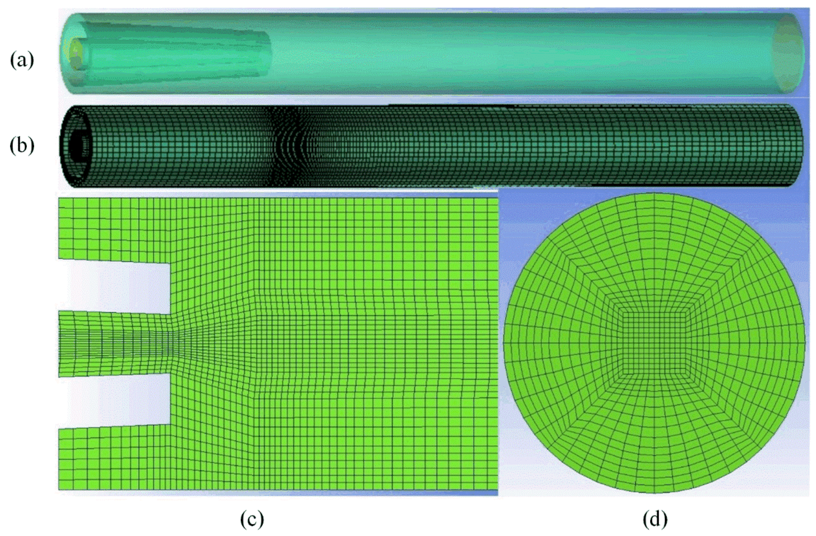
2.2. Simulation Zone and Grid Solution

To ensure high-quality grid generation, an O-block structure mesh was utilized using ICEM software, as depicted in Figure 3. Grid quality plays a crucial role in achieving convergence in simulations, and the grid quality in this study exceeded 0.7. In numerical simulations, mesh density refers to the number of grid or mesh points used to discretize the computational domain. The mesh is a network of interconnected cells or elements that approximate the continuous domain being simulated. The choice of mesh density plays a crucial role in determining the accuracy and computational efficiency of the simulation. Due to the significant changes in physical parameters around the interphase, the grid density used in this study was increased, resulting in relatively large aspect ratios. Figure 3c,d illustrates a sectional view and a partially enlarged view of the mesh, which provide a more detailed visualization of the mesh’s structural elements.

2.3. Model Settings and Boundary Conditions

Regarding the solution setup, a double-precision steady-state solver was utilized for the numerical computation. Except for the turbulence equations, which were solved by using a first-order upwind differencing scheme, higher-order differencing schemes were employed for all other equations. Iterative convergence was achieved when the residuals of all conservation equations were less than 1 × 10⁻⁵, and the inlet pressure of the primary and secondary flows remained constant after monitoring. All calculations were performed on a computer with 44-core CPUs and 128 GB memory. The computation time for each operating condition was approximately 30 h.
In numerical simulations, the appropriate boundary conditions play a crucial role in the computation results. The inlet boundary conditions for the primary flow consist of a mass flow rate inlet and a temperature inlet corresponding to the saturation pressure of the steam. The inlet conditions for the secondary flow are also specified as a mass flow rate inlet boundary condition. The outlet of the mixed hot water is specified as an open pressure boundary condition, with a relative pressure of zero and a return flow of water. All wall boundaries are modeled as adiabatic no-slip conditions. The thermophysical properties were obtained from the IAPWS-IF97 substance group.

2.4. Condensation Model

A numerical model based on the Eulerian–Eulerian multiphase model has been developed to accurately simulate the characteristics of pressure profile along the axial direction in subcooled water flow in a pipe. The model considers each phase as having its own separate set of conservation equations, governing the equilibrium of mass, momentum, and energy [23]. In cases where one phase is continuous and the other is dispersed, a particle model is available. The particle model has been employed for interphase transfer. The interphase heat and mass transfer have been calculated using CFX Expression Language (CEL) based on a thermal phase change model. The continuous and dispersed phases are denoted as the primary and secondary phases, respectively, with liquid water α as the continuous phase and steam β as the dispersed phase. A more detailed explanation of the particle model can be found in ref. [24]. The related description for the present condensation model can be accessed in our previously published study [25].

2.5. Grid Independency and Model Validation

To verify the independence of computational results from the number of grids, a total of three different numbers of grids were planned for the independence test. Figure 4 shows the axial static pressure profile under the conditions of mβ = 0.001 kg/s, Tβ = 376 K, mα = 0.05 kg/s, and Tα = 300 K. The ordinate represents static pressure, and the abscissa represents axial position. When the number of grids is 115,335 and 249,945, the axial static pressure profile is basically identical. In order to ensure computational accuracy and reduce time costs, the grid with a quantity of 115,335 was selected as the final grid solution.
For the validation of model accuracy, numerical simulation results were compared with experimental results [22]. As shown in Figure 5, the gas volume fraction profile obtained from the simulation was compared with the steam plume captured in the experiment under the conditions of Ge = 509 kg/(m2·s), Tw = 5.9 °C, and Re = 28,014, with the same boundary conditions as the original experiment. The main comparison objects were the shape and penetration length of the steam plume. In order to compare the target steam plume area, only a local area was displayed. It was found that the shape of the steam plume obtained from the simulation was similar to that captured by the high-speed camera used in this paper, and both showed a conical shape. In the experiment, the length of the steam plume is often determined by the brightness change at the liquid–vapor interface, while in the numerical simulation, it is determined by the void fraction profile. The axial boundary of the steam plume penetration is determined at the point where the gas volume fraction V = 0.999, and it was observed that the steam plume penetration lengths were basically consistent through the void fraction cloud map.
In addition to comparing the size and shape of the steam plume, the temperature profile of the simulation and experiment was further compared. As shown in Figure 6, the temperature profile along the nozzle axis was compared, where X represents the distance from the nozzle inlet. It was found that the temperature change trend obtained by the numerical calculation method was consistent with the experimental results, and the two were in good agreement. Therefore, by comparing both qualitatively and quantitatively, the numerical simulation results and experimental data were consistent, demonstrating that this model can predict the condensation characteristics of steam jets in flowing water inside pipes effectively.

3. Results and Discussion

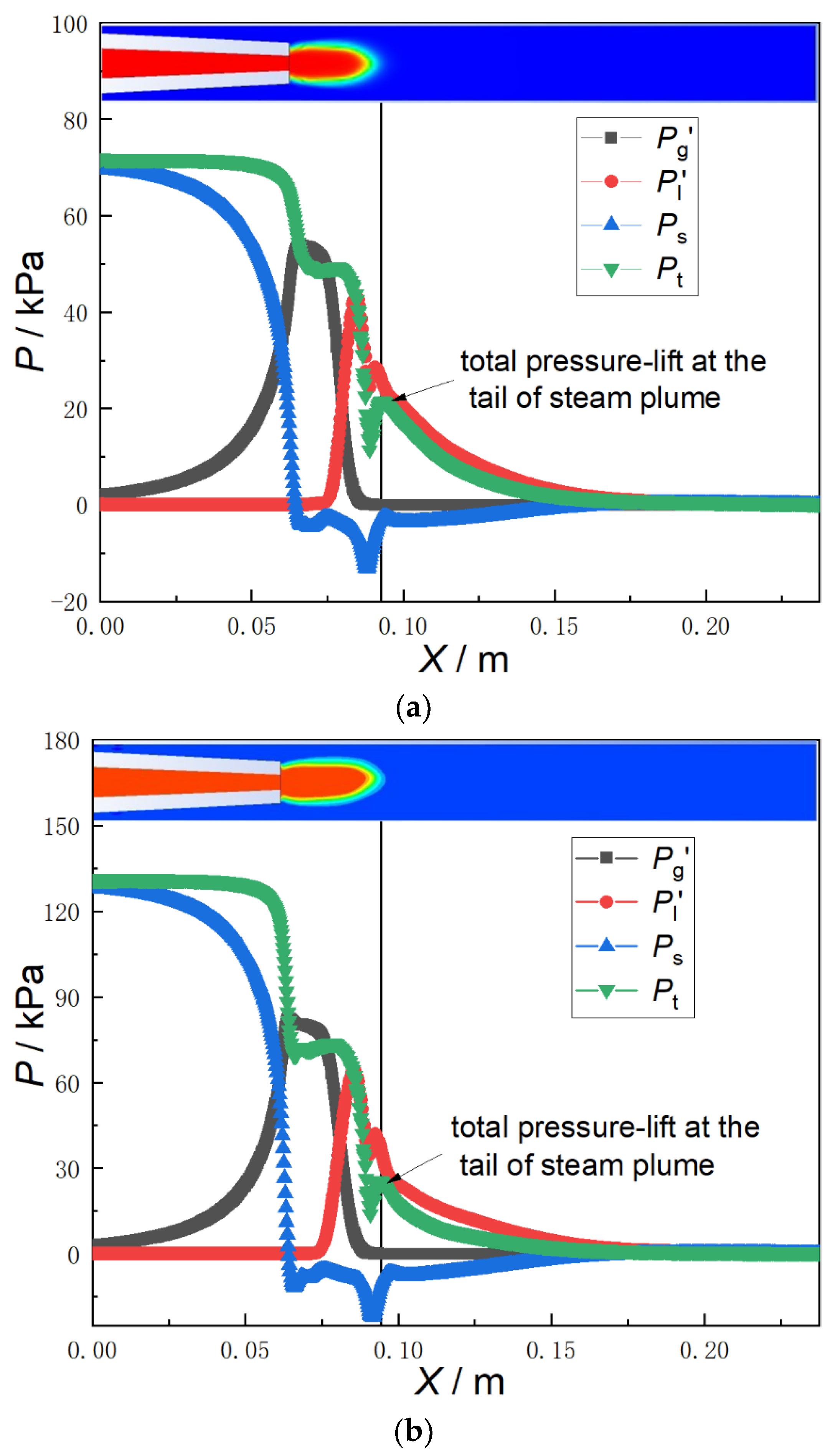
3.1. Profile of the Total Pressure

To unravel the enigma behind steam plume, Wu [20] utilized a Pitot tube to measure the total pressure and found that a pressure jump was caused by condensation shock. This enabled them to obtain the numerical profile of total pressure. In this study, the total pressure profile characteristics of steam jet inside the pipe using numerical method was investigated. The total pressure profile at any position in the flow field can be directly exported using ANSYS CFX-POST. Figure 7 presents the axial total pressure profile and gas volume fraction cloud map under six different operating conditions. The pressure distribution is influenced not only by the steam mass flux and subcooled water temperature but also by the Reynolds number of the water flow (Re = 4Q/μπD). It is observed that a pressure jump phenomenon, known as condensation shock wave, appears in the total pressure profile at the end of the steam plume, i.e., at the end of condensation. Due to the fact that total pressure is composed of three components, namely static pressure, steam dynamic pressure, and water dynamic pressure, the axial profile of these pressures will be compared below in order to identify the main factors that cause a sudden jump in total pressure at the trailing edge of the plume.

3.2. The Relationship between Total Pressure, Static Pressure and Dynamic Pressure

When conducting experiments, it can be challenging to obtain accurate measurements for dynamic pressure. However, numerical methods can provide us with this information. Therefore, the present section will focus primarily on dynamic pressure of steam and water.
It is noteworthy that it is not possible to obtain total pressure by postprocessing of the Eulerian multiphase model. However, it can be calculated using Equation (13), which involves the summation of the static pressure, dynamic pressure of steam and water.
Pt = Ps + Pd
where Ps and Pd represent static pressure and dynamic pressure, respectively.
P d = Φ P g + ( 1 Φ ) P 1
P g = 1 2 ρ g V g 2
P 1 = 1 2 ρ 1 V 1 2
For a grid cell consisting of pure gas or pure liquid phase, its dynamic pressure can be calculated according to the above equation. However, in this study, the dynamic pressure of two-phase flow is calculated, where a grid cell contains both gas and liquid phases. Here, the gas volume fraction Φ is introduced, and the dynamic pressure of the gas phase in a grid cell is ΦPg, while the dynamic pressure of the liquid phase is (1 − Φ)Pl. The sum of these two quantities yields the total dynamic pressure.
Figure 8 displays the profile of dynamic pressures for axial total pressure, static pressure, steam, and liquid water. The dynamic pressure of steam is denoted by Pg′, with a value of ΦPg, while the dynamic pressure of the liquid phase is denoted by Pl′, with a value of (1 − Φ)Pl.
Based on the four variations observed, it can be concluded that the sudden jump in total pressure at the end of the steam flow corresponds to a sudden jump in water dynamic pressure at the same location. Additionally, a sudden jump in static pressure occurs at this point, suggesting that the sudden jumps in static pressure and water dynamic pressure are the main cause of the sudden jump in total pressure. Furthermore, it is observed that water dynamic pressure exceeds total pressure due to the negative static pressure at the location of the pressure jump.

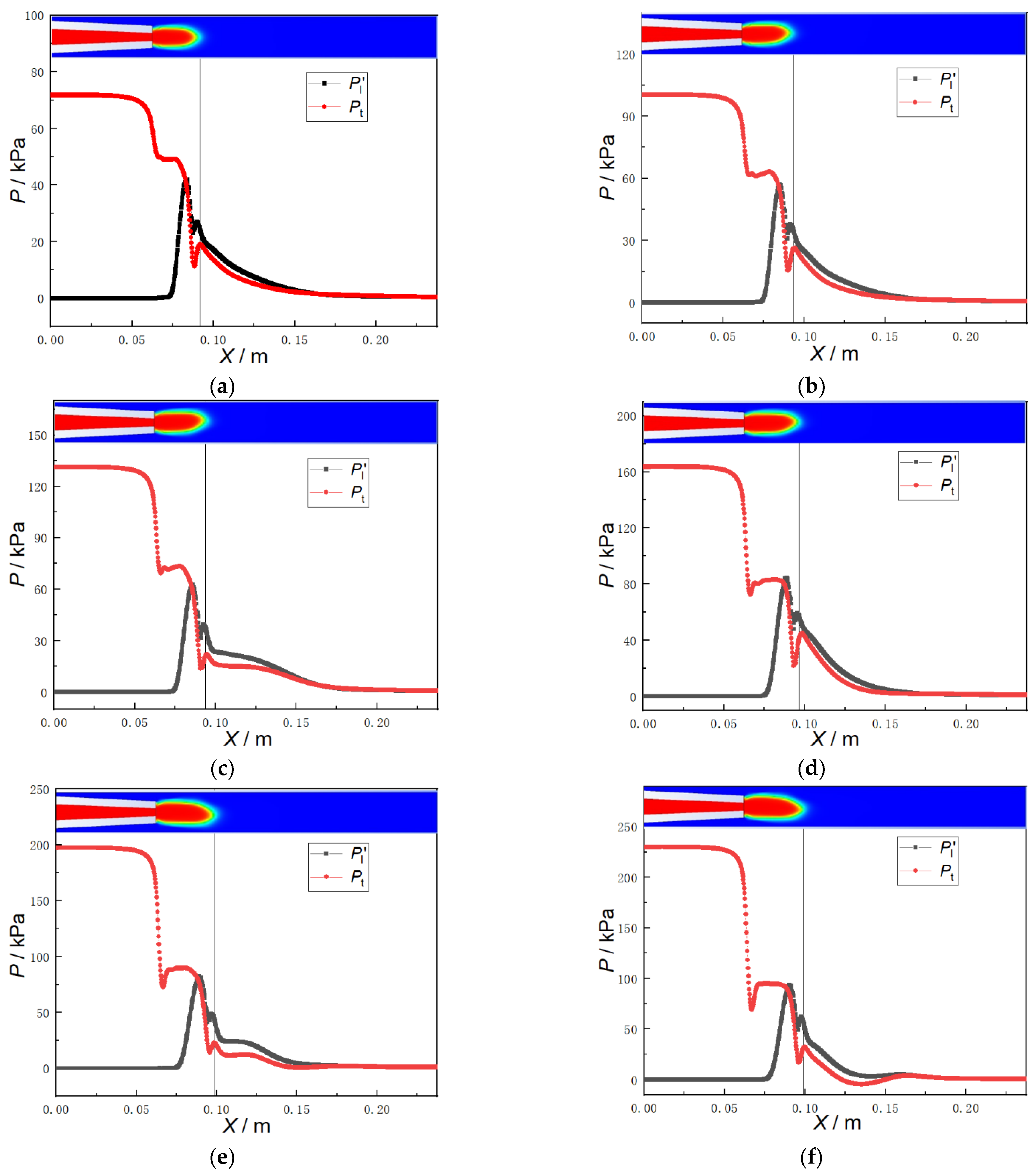
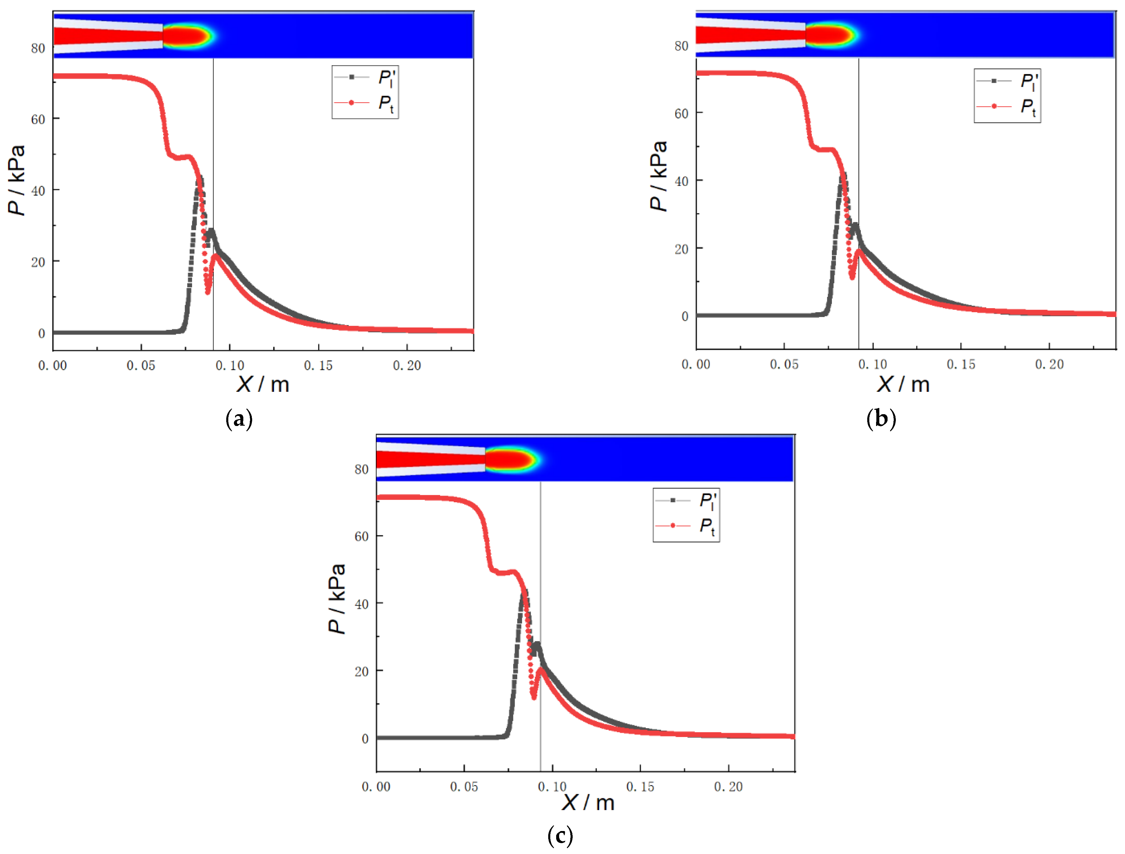
3.3. The Peak of Water Dynamic Pressure

To investigate whether the dynamic pressure jump of water at the trailing edge of the steam plume is the main cause of the total pressure jump, a comparison was made between the total pressure and the dynamic pressure of water with varying steam inlet pressures at Tw = 16.85 °C and Re = 26,200, as shown in Figure 9.
From Figure 9, it was observed that at six different steam inlet pressures, namely Pin = 71 kPa, 100 kPa, 130 kPa, 163 kPa, 200 kPa, and 226 kPa, both the total pressure and the dynamic pressure of water exhibited pressure jumps simultaneously at the trailing edge of the steam plume. This indicates that the total pressure jump at the trailing edge of the steam plume is caused by the dynamic pressure jump of water.
In order to quantitatively further compare the influences of steam inlet pressure on the dynamic pressure and total pressure of water at the trailing edge of a steam jet plume, a vertical line was drawn at the trailing edge of the steam jet plume, which precisely intersected with the peak values of the dynamic pressure of water and total pressure. Both the total pressure peak value and the dynamic pressure peak value of water increase with the increase in the inlet pressure, which is consistent with the experimental results of Wu et al. [21]. Combined with the changes of the steam plume with the variation in the steam inlet pressure, the positions of the total pressure peak value and the dynamic pressure peak value of water at the trailing edge of the steam plume both move downstream with the increase in the steam inlet pressure.
Figure 10 compares the profile of water dynamic pressure and total pressure along the axis at different water temperatures, with inlet temperatures of 6.85 °C, 16.85 °C, and 26.85 °C, respectively. When observing the profile of axis total pressure and water dynamic pressure under these three water temperature conditions, it is found that there is a pressure jump phenomenon at the trailing edge of the steam plume. The vertical line marked in Figure 10 quantitatively further compares the effect of inlet water temperature on the peak values of total pressure and water dynamic pressure after the pressure jump at the trailing edge of the steam plume. It is found that as the water inlet temperature increases, both the peak values of water dynamic pressure and total pressure decrease. Similar trends were also observed by Wu et al. [20] in their experiments.
The pressure profile characteristics of submerged steam jets in water flow in a narrow pipe are not only influenced by the steam inlet pressure and water inlet temperature, but also by the Reynolds number of water flow. Figure 11 shows the variation trends of the total pressure and the dynamic pressure of water with the Reynolds number of water flow at three different Reynolds numbers (Re = 9500, 19,800, and 25,000). It is observed that under different conditions of Reynolds number of water flow, pressure jumps occur in both the total pressure and dynamic pressure of water at trailing edge of steam plume.

4. Conclusions

In this paper, a three-dimensional steady CFD simulation was carried out to investigate the pressure profile of submerged steam jet in subcooled water flow in a narrow pipe. The numerical results show that the shape of the steam plume and the axial temperature profile are in good agreement with the experimental data. This validates the correctness of the numerical model both qualitatively and quantitatively. Furthermore, the numerical simulation was conducted under various steam inlet pressures, water inlet temperatures, and the Reynolds number of water flow. The main results could be summarized as follows:
  • By analyzing the axial total pressure profile and gas volume fraction contour, it was found that a pressure jump phenomenon, known as condensation shock wave, occurred in the total pressure profile corresponding to the tail of the steam plume.
  • The sudden increase in total pressure at the location of condensation completion, observed at the trailing edge of steam plume, is accompanied by a similar sudden rise in dynamic pressure of the subcooled water. Therefore, it can be inferred that the sudden rise in dynamic pressure of the water is the primary cause of the observed total pressure jump at the trailing edge of steam plume.
  • The peak of water dynamic pressure was discussed under different steam inlet pressures, water inlet temperatures, and the Reynolds number of water flow, further validating that the dynamic pressure rise of subcooled water is the cause of total pressure rise.

Author Contributions

Methodology, X.C. and L.T.; software, X.C. and J.Z.; validation, L.F. and S.J.; formal analysis, X.C. and B.L.; investigation, X.C. and L.S.; resources, L.F. and S.J.; data curation, X.C. and J.Z.; writing—original draft preparation, X.C.; writing—review and editing, X.C., L.F., S.J., J.Z. and L.T.; visualization, X.C., L.S. and B.L.; supervision, B.L. and L.T. All authors have read and agreed to the published version of the manuscript.

Funding

This research was funded by the Open Fund of Science and Technology on Thermal Energy and Power Laboratory (TPL2020B02 and TPL2020B04), Doctoral Research Fund of Shandong Jianzhu University (X20035Z), the Plan of Guidance and Cultivation for Young Innovative Talents of Shandong Provincial Colleges and Universities, and the Natural Science Basic Research Plan of Shaanxi Province of China (2023-JC-YB-350 and 2021JQ-578).

Data Availability Statement

The data that support the findings of this study are available from the first author.

Conflicts of Interest

The authors declare no conflict of interest.

References

  1. Madejski, P.; Kuś, T.; Michalak, P.; Karch, M.; Subramanian, N. Direct Contact Condensers: A Comprehensive Review of Experimental and Numerical Investigations on Direct-Contact Condensation. Energies 2022, 15, 9312. [Google Scholar] [CrossRef]
  2. Mahood, H.B.; Campbell, A.N.; Thorpe, R.B.; Sharif, A.O. Experimental measurements and theoretical prediction for the volumetric heat transfer coefficient of a three-phase direct contact condenser. Int. Commun. Heat Mass Transf. 2015, 66, 180–188. [Google Scholar] [CrossRef] [Green Version]
  3. Baqir, A.S.; Mahood, H.B.; Sayer, A.H. Temperature distribution measurements and modelling of a liquid-liquid-vapour spray column direct contact heat exchanger. Appl. Therm. Eng. 2018, 139, 542–551. [Google Scholar] [CrossRef]
  4. Barton, P.T.; Obadia, B.; Drikakis, D. A conservative level-set based method for compressible solid/fluid problems on fixed grids. J. Comput. Phys. 2011, 230, 7867–7890. [Google Scholar] [CrossRef]
  5. Gulawani, S.S.; Joshi, J.B.; Shah, M.S.; RamaPrasad, C.S.; Shukla, D.S. CFD analysis of flow pattern and heat transfer in direct contact steam condensation. Chem. Eng. Sci. 2006, 61, 5204–5220. [Google Scholar] [CrossRef]
  6. Shah, A.; Chughtai, I.R.; Inayat, M.H. Experimental study of the characteristics of steam jet pump and effect of mixing section length on direct-contact condensation. Int. J. Heat Mass Transf. 2013, 58, 62–69. [Google Scholar] [CrossRef]
  7. Shah, A.; Chughtai, I.R.; Inayat, M.H. Experimental and numerical investigation of the effect of mixing section length on direct-contact condensation in steam jet pump. Int. J. Heat Mass Transf. 2014, 72, 430–439. [Google Scholar] [CrossRef]
  8. Zhou, L.; Chen, W.; Chong, D.; Liu, J.; Yan, J. Numerical investigation on flow characteristic of supersonic steam jet condensed into a water pool. Int. J. Heat Mass Transf. 2017, 108, 351–361. [Google Scholar] [CrossRef]
  9. Zhou, L.; Liu, J.; Chong, D.; Yan, J. Numerical analysis on pressure profile for sonic steam jet condensed into subcooled water. Int. J. Heat Mass Transf. 2016, 99, 53–64. [Google Scholar] [CrossRef]
  10. Qu, X.; Sui, H.; Tian, M. CFD simulation of steam–air jet condensation. Nucl. Eng. Des. 2016, 297, 44–53. [Google Scholar] [CrossRef]
  11. Qu, X.; Revankar, S.T.; Tian, M. Numerical simulation of bubble formation and condensation of steam air mixture injected in subcooled pool. Nucl. Eng. Des. 2017, 320, 123–132. [Google Scholar] [CrossRef]
  12. Qu, X.; Tian, M.; Zhang, G.; Leng, X. Experimental and numerical investigations on the air–steam mixture bubble condensation characteristics in stagnant cool water. Nucl. Eng. Des. 2015, 285, 188–196. [Google Scholar] [CrossRef]
  13. Patel, G.; Tanskanen, V.; Kyrki-Rajamäki, R. Numerical modelling of low-Reynolds number direct contact condensation in a suppression pool test facility. Ann. Nucl. Energy 2014, 71, 376–387. [Google Scholar] [CrossRef]
  14. Tanskanen, V.; Jordan, A.; Puustinen, M.; Kyrki-Rajamäki, R. CFD simulation and pattern recognition analysis of the chugging condensation regime. Ann. Nucl. Energy 2014, 66, 133–143. [Google Scholar] [CrossRef]
  15. Li, S.; Wang, P.; Lu, T. Numerical simulation of direct contact condensation of subsonic steam injected in a water pool using VOF method and LES turbulence model. Prog. Nucl. Energy 2015, 78, 201–215. [Google Scholar] [CrossRef]
  16. Chan, C.K.; Lee, C.K.B. A regime map for direct contact condensation. Int. J. Multiph. Flow 1982, 8, 11–20. [Google Scholar] [CrossRef]
  17. Kim, H.Y.; Bae, Y.Y.; Song, C.H.; Park, J.K.; Sang, M.C. Experimental study on stable steam condensation in a quenching tank. Int. J. Energy Res. 2001, 25, 239–252. [Google Scholar] [CrossRef]
  18. Del Tin, G.; Lavagno, E.; Malandrone, M. Experimental Study on Steam Jet Condensation in Subcooled Water Pool. In Multi-Phase Flow and Heat Transfer Symposium-Workshop. 3; University of Miami: Coral Gables, FL, USA, 1983; pp. 134–136. [Google Scholar]
  19. Yan, J.; Wu, X.; Chong, D. Experimental study on pressure and temperature distributions for low mass flux steam jet in subcooled water. Sci. China Technol. Sci. 2009, 52, 1493–1501. [Google Scholar] [CrossRef]
  20. Wu, X.; Yan, J.; Li, W.; Pan, D.; Liu, G. Experimental study on a steam-driven turbulent jet in subcooled water. Nucl. Eng. Des. 2010, 240, 3259–3266. [Google Scholar] [CrossRef]
  21. Wu, X.; Li, W.; Yan, J. Research on axial total pressure profiles of sonic steam jet in subcooled water. Nucl. Power Eng. 2012, 33, 76–80. (In Chinese) [Google Scholar]
  22. Chen, X.; Tian, M.; Zhang, G.; Leng, X.; Qiu, Y.; Zhang, J. Visualization study on direct contact condensation characteristics of sonic steam jet in subcooled water flow in a restricted channel. Int. J. Heat Mass Transf. 2019, 145, 118761. [Google Scholar] [CrossRef]
  23. Ishii, M.; Hibiki, T. Thermo-Fluid Dynamics of Two-Phase Flow; Springer: New York, NY, USA, 2010. [Google Scholar]
  24. ANSYS®. Academic Research, Release 15.0, Help System. In ANSYS CFX-Solver Theory Guide; ANSYS Inc.: Canonsburg, PA, USA, 2013. [Google Scholar]
  25. Chen, X.; Tian, M.; Qu, X.; Zhang, Y. Numerical investigation on the interfacial characteristics of steam jet condensation in subcooled water flow in a restricted channel. Int. J. Heat Mass Transf. 2019, 137, 908–921. [Google Scholar] [CrossRef]
Figure 1. Schematic diagram of experimental system.
Processes 11 01821 g001
Figure 2. Dimensions of the test section.
Processes 11 01821 g002
Figure 3. Simulation domain and mesh. (a) Schematic model of simulation domain. (b) Overall geometry showing external surface mesh. (c) Local mesh detail in axial section. (d) Local mesh detail in radial section.
Processes 11 01821 g003
Figure 4. Mesh independency check, when mβ = 0.001 kg/s, Tβ = 376 K, mα = 0.05 kg/s, and Tα = 300 K.
Processes 11 01821 g004
Figure 5. Comparison of gas volume fraction between experiment [22] and simulation when Ge = 509 kg/(m2·s), Tw = 5.9 °C, and Re = 28,014.
Processes 11 01821 g005
Figure 6. Comparison of axial temperature profiles between simulation and experiment [16], Ge = 509 kg/(m2·s), Tw = 5.9 °C, and Re = 28,014.
Processes 11 01821 g006
Figure 7. The profile of total pressure along axial location. (a) Ge = 255 kg/(m2·s), Tw = 6.85 °C, and Re = 19,800; (b) Ge = 306 kg/(m2·s), Tw = 6.85 °C, and Re = 23,850; (c) Ge = 407 kg/(m2·s), Tw = 26.85 °C, and Re = 28,050; (d) Ge = 458 kg/(m2·s), Tw = 42 °C, and Re = 28,050.
Processes 11 01821 g007
Figure 8. The profiles of total pressure, static pressure and dynamic pressure along axial direction. (a) Ge = 255 kg/(m2·s), Tw = 6.85 °C, and Re = 19,800; (b) Ge = 356 kg/(m2·s), Tw = 6.85 °C, and Re = 26,020.
Processes 11 01821 g008
Figure 9. The comparison between total pressure and the dynamic pressure of water along axial direction under different steam inlet pressures, Tw = 16.85 °C and Re = 26,200. (a) Ge = 255 kg/(m2·s) and Pin = 71 kPa; (b) Ge = 306 kg/(m2·s) and Pin = 100 kPa; (c) Ge = 356 kg/(m2·s) and Pin = 130 kPa; (d) Ge = 407 kg/(m2·s) and Pin = 163 kPa; (e) Ge = 458 kg/(m2·s) and Pin = 200 kPa; (f) Ge = 508 kg/(m2·s) and Pin = 226 kPa.
Processes 11 01821 g009
Figure 10. The comparison between total pressure and dynamic pressure of water along the axis under different water temperatures. (a) Tin = 6.85 °C; (b) Tin = 16.85 °C; (c) Tin = 26.85 °C.
Processes 11 01821 g010
Figure 11. The comparison between total pressure and dynamic pressure of water along the axis under different Reynolds numbers of waterflow. (a) Re = 9500; (b) Re = 19,800; (c) Re = 25,000.
Processes 11 01821 g011
Disclaimer/Publisher’s Note: The statements, opinions and data contained in all publications are solely those of the individual author(s) and contributor(s) and not of MDPI and/or the editor(s). MDPI and/or the editor(s) disclaim responsibility for any injury to people or property resulting from any ideas, methods, instructions or products referred to in the content.

