Abstract
This study investigates the Hagen–Poiseuille pipe flow of viscoplastic fluids, focusing on analytical predictions of concrete pumping using the shear-stress-dependent parabolic model, extending analytical studies to a nonlinear rheological model with easily accessible experimental parameters. Research novelty and highlights encompass solving the steady laminar pipe flow for viscoplastic fluids described by the parabolic model, presenting detailed results for the two-fluid parabolic model, and introducing a computational app implementing theoretical findings. The parabolic model outperforms linear models, such as the Bingham model, in accuracy by accounting for the nonlinearity in the flow curves (i.e., shear stress and shear rate relations) of pumped concrete. The influence of rheological parameters on these relations is analyzed, and their versatility is demonstrated by a Wolfram Mathematica-based application program. The analytical approach developed in this work is adaptable for other models with shear stress as the independent variable, offering valuable insights into viscoplastic fluid flows.
1. Introduction
Viscoplastic fluids are a type of non–Newtonian fluid that exhibit yield stress. For these fluids to flow, applied stress must exceed a critical value known as ”yield stress“ [1,2,3,4,5,6]. The yield stress is therefore characterized as the material’s resistance to the initiation of flow. According to historical records [1], viscoplasticity was first discovered in the 1890s by Schwedoff when he used a Couette instrument to perform experiments on colloidal gelatin solutions. His findings revealed a nonlinear relationship between the torque and angular velocity in this instrument, making his experiments be the first set of measurements of non-Newtonian behavior. To describe his results, he had to include a yield stress value. Following this, the work of Bingham and Green in the 1920s led to broad acknowledgment that some fluids display yield stress behavior [1,7,8,9]. Many industrially important materials, such as concentrated suspensions [10,11], red mud residues [12], pastes [13], food products [14], emulsions [15], foams [16], waxy crude oils [17], fiber-reinforced plastics [18], and other composites, are viscoplastic. Concrete is another example of viscoplastic fluid [19,20,21,22], and is the most widely used man-made material in the world. It is indispensable for numerous major infrastructure developments, from buildings, roads, bridges, and high-speed rail facilities to renewable energy applications.
Concrete pumping is a common placement technique that makes it possible to deliver concrete considerably more quickly, which speeds up construction and thus reduces costs [23,24,25]. At the same time, the effective application of pumping technology can offer excellent reliability and productivity during the construction process while reducing the danger of failure involving human error. Therefore, there is a significant economic benefit to understanding and precisely defining the pumping behavior of concrete [25]. However, pumping concrete is not a simple process, and many accidents occur every year as a result of pump or pipeline blockages, blowouts, or breaks [23,24]. Consequently, a prior prediction of concrete flow rates, which influence construction process duration, is required to apply concrete pumping to large-scale construction projects [26].
Using known rheological models, several attempts have been made to estimate concrete flow in pumping. The majority of approaches to concrete pumping have considered the yield stress and the presence of the unsheared zone by presuming that concrete behaves as a Bingham fluid or Herschel–Bulkley fluid. However, without taking into account the fact that there is a lubricating layer at the interface between the concrete and the pipe, these approaches nearly always failed to correctly estimate pumping flow rate on a wide range of concrete fluidities [26]. The possible mechanisms that contribute to the formation of the lubrication layer (LL) include the wall effect phenomenon caused by particle–wall interactions and shear-induced particle migration (SIPM) [27,28,29,30,31,32].
Kaplan et al. [33,34] conducted a pioneering study on predicting pumping performance, which proved that the lubricating layer is important in facilitating concrete pumping because it has much lower viscosity and yield stress than concrete [30,31]. In 2013, Kwon et al. [31,35], followed by Khatib and Khayat [36], developed analytical predictions on concrete pumping that included the rheological properties of the lubrication layer fluid. Prior theoretical works of Kaplan [33], Kwon et al. [35], and Khatib and Khayat [36] used the classical Bingham model to characterize the rheological behavior of bulk concrete and the lubrication layer fluid, which sets a linear relationship between shear stress () and shear rate (), given by
where and are the two parameters of the Bingham model: yield stress and plastic viscosity, respectively.
Although the Bingham model is frequently used for cement-based materials, it has been extensively reported that the relationship between shear stress and shear rate for fresh concrete, mortar, and cement paste is not exactly linear [20,37,38,39,40]. Because the Bingham model does not account for this non-linearity, two commonly used rheological models to describe the shear-thickening behavior of fresh self-compacting concrete are the Herschel–Bulkley and the modified Bingham models [37,38,40]. Recently, Zhaidarbek et al. [41] developed a flow rate–pressure drop relation for both dual-fluid Herschel–Bulkley and the dual-fluid modified Bingham models, where the two fluids are bulk concrete and the lubrication layer fluid. The constitutive equation for the Herschel–Bulkley model is given by [41]
which has three parameters: yield stress, , flow consistency index, , and flow behavior index (dimensionless), . For , the fluid is shear-thinning, and for , the fluid is shear-thickening. If , the Herschel–Bulkley fluid model reduces to the Bingham model with plastic viscosity .
The constitutive equation of the modified Bingham model is given by [41]
which also has three parameters: yield stress, , plastic viscosity, , and a second-order coefficient, , that describes the deviations from the linear relation between shear stress and shear rate as described by the Bingham model in Equation (1). For , the modified Bingham model shows a shear-thickening behavior, and for , the model displays a shear-thinning behavior. Similarly, for , the modified Bingham model reduces to the Bingham model in Equation (1).
Although there seems to be a sufficient study on the pumping behavior of concrete and lubrication layer properties based on nonlinear rheological models, the proposed models can be difficult to employ in rheological experiments. As shown by Li et al. [42], by solving the Couette inverse program, the resulting relationships between torque and rotational speed in a coaxial cylinder rheometer for the Herschel–Bulkley model and the modified Bingham model are rather bulky and are difficult to apply in regression analysis of experimental data. In comparison, the shear-stress-dependent Parabolic model, which contains a nonlinear term between shear stress and shear rate, has a resulting torque–angular frequency relation described by a simple quadratic function with easy-to-access parameters. Therefore, according to Li et al. [42], among all the commonly used three-parameter rheological models for yield-stress fluids, the parabolic model is the most suitable for the analysis of the torque–angular frequency data from a rotational rheometer.
The parabolic model was first introduced in 1985 by Atzeni et al. [43] as a parabolic-type empirical law that relates the shear rate to the stress as
It was noted that the parabolic model offered a good fit with the experimental data along with the Herschel–Bulkley and Eyring models, and important rheological parameters such as yield stress () and viscosity () can easily be derived with this model. Li et al. [42] emphasized that the parabolic model’s introduction as an inverse function makes it easier to solve the Couette inverse problem based on this model, which deals with the relationship between rotational speed and torque. In a more recent study [44], the modified Bingham model and the parabolic model were compared, and the results showed that the parabolic model provided a more precise characterization of the paste’s flowing performance. The rheological parameters for pastes obtained based on the modified Bingham model lacked credibility in comparison to the parabolic model.
Traditionally, most of the constitutive models use shear rate as the independent variable and are expressed in the form of . However, such constitutive models may also be expressed in the form of by finding their inverse functions. There are models, such as the Ellis model [45], the Meter model [46], and the Parabolic model [43], that are commonly expressed in the form of using the shear stress as the independent variable. Among them, the parabolic model has yield stress and can describe viscoplastic fluids such as cement pastes [42,43,44,47].
Despite the listed advantages of the parabolic model over other commonly used three-parameter rheological models, studies on the shear-stress-dependent parabolic model [42,43,44,47] are scarce. In particular, there is a lack of detailed analysis of the parabolic model, and, to the best of our knowledge, the pipe flow problem of the parabolic fluid has not been solved so far either for the single- or the dual-fluid case. The main nolvety and research objectives of this paper are to: (i) Develop a theoretical framework suitable for solving the Hagen–Poiseuille pipe flow problem for viscoplastic fluids with shear-stress-dependent constitutive models; (ii) Advance the state-of-the-art in rheology-based analytical models for predicting flow rate vs. pressure drop relationships in concrete pumping; and (iii) Using the parabolic model as a representative case, solve the associated Hagen–Poiseuille pipe flow problem and develop analytical models for concrete pumping predictions.
2. Theoretical Framework and Derivations
2.1. Analysis of the Parabolic Model
Generally speaking, constitutive models for incompressible viscoplastic fluids can be classified as those using the shear rate as the independent variable, i.e., , and those using the shear stress as the independent variable, i.e., . While it is a common practice to introduce the viscosity function (SI unit: ) as
for the former class of constitutive models, it is more convenient to introduce the fluidity function (SI unit: ) [1,48] as
for the latter class of constitutive models.
The term in Equation (4) with coefficient c brings in nonlinear dependence of the shear rate on the shear stress when . A careful analysis of the model shows that the fluid is a Bingham plastic if , yield-pseudoplastic (i.e., shear thinning) if , and is yield-dilatant (also referred to as shear-thickening) if , as shown in Figure 1.
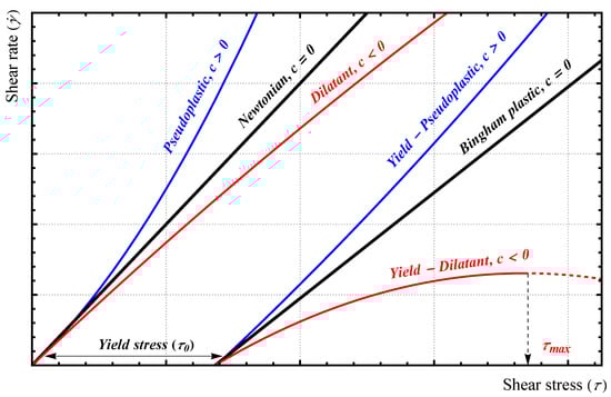
Figure 1.
Graphical representation of the different scenarios described by the parabolic model given in Equation (7).
From Figure 1, the correct form of the parabolic model should be expressed as
where is the yield stress and is obtained by requiring the shear rate given by Equation (7) to be a continuous function. We have
The above expression requires . The term in Equation (7) corresponds to an upper limit in the shear stress required by the model for the case of , and
Note that is equivalent to saying that there is no restriction on the upper limit of shear stress in the model. Moreover, note that at , we have , i.e., the fluid does not have a yield stress.
Table 1 presents the SI units and dimensions in terms of the MLT (i.e., Mass, Length, and Time) system associated with the variables and parameters of the parabolic model. The parabolic model, given in Equation (7), belongs to the class of constitutive models that use the shear stress as the independent variable, and its fluidity function is given by

Table 1.
The SI units and dimensions in terms of the MLT (i.e., Mass, Length, and Time) system associated with the variables and parameters of the parabolic model.
In the case of , the parabolic model reduces to the classical Bingham model with yield stress and plastic viscosity , where
Thus, it is required that and for the model to be of practical use.
Presented here is the ratio between the true yield stress of the parabolic model, , and :
where is a dimensionless number defined as
In the case of , we have and . The relationship between vs. for is shown in Figure 2.
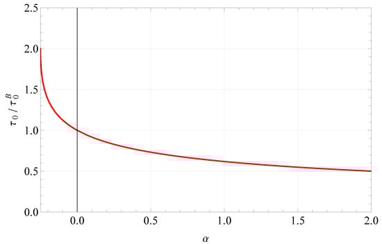
Figure 2.
Relationship between the true yield stress of the parabolic model and the dimensionless number, .
2.2. Hagen–Poiseuille Equation for Non-Newtonian Pipe Flow: Single Fluid
The Hagen–Poiseuille equation is a physical law that gives the pressure drop in an incompressible Newtonian fluid in laminar flow flowing through a long cylindrical pipe of a constant cross-section [49]. This section will introduce the general method for obtaining the Hagen–Poiseuille equation for constitutive models that use shear stress as the independent variable.
Let G be the pressure drop per unit length of the pipe, i.e.,
where is the pressure drop; and are, respectively, the “modified” pressures [50] at and . From the basics of pipe flow, the distribution of shear stress is obtained as [50]
Here, is the pressure drop per unit length of the pipe given by Equation (14). From Equation (15) the shear stress at the pipe wall (where ) is obtained as
For the parabolic model, the wall shear rate is given as
The yield radius, also called “plug” radius, can be determined by solving the equation of for r, as follows:
In the region of , the fluid exhibits a constant velocity across the cross-section that is perpendicular to the pipe’s axis, thus, corresponding to the plug flow zone.
According to its definition, the volumetric flow rate can be obtained from the velocity distribution as
Carrying out the integration by parts yields
Assuming the no-slip velocity at the wall of the tube, i.e., , the first term on the right-hand side of Equation (20) is zero at both limits of the integration. Thus, we have
In the plug-flow region, , we have . In the shear-flow region, , we have , which, for the parabolic model, can be expressed as a function of the shear stress, . For the Hagen–Poiseuille flow in a pipe, we have a linear shear stress distribution of the form:
Thus, we have and . Substituting the expression for r and into Equation (21), the volumetric flow rate is now given by
After simplification, we have
where the variable of integration is the shear stress, , and the shear rate, expressed as a function of the shear stress, depends on the rheological properties of the fluid; is the fluidity function, as introduced in Equation (6).
Introducing the dimensionless variables given in Table 2 to simplify the expressions, the shear rate and integral in Equation (24) can be rewritten as
where dimensionless plug radius is found using the definitions of yield and wall shear stresses:
Table 2.
Nondimensionalization used in this work, following the same approach as that used in our recent work [51].
The Hagen-Poiseulle equation for the single fluid case using the parabolic model in terms of dimensionless variables summarized in Table 2 is thus calculated from
where is given by Equation (17) and is given by Equation (26).
From Equation (26), the dimensionless average velocity for the parabolic model is found to be
By subsititing the a, b parameters from Table 2 and setting , Equation (28) reduces to the Hagen–Poiseuille equation for the Bingham model as
By substituting and Bingham model parameters given in Equation (11), Equation (30) can be rewritten as
where as given in Equation (16). Equation (31) is known as the Buckingham–Reiner Equation [50,52].
The same flow rate–pressure drop relation can be obtained using a more traditional approach, namely, by integrating the velocity distribution. For the parabolic model, the governing ordinary differential equations (ODEs) for bulk concrete in shearing flow region, where , and plug flow region, where , are given by
Introducing and (see Table 2), Equation (32) may be rewritten as
By solving Equation (32) with the no-slip boundary condition at the wall, i.e., , and at plug flow/shearing flow interface, the velocity profile at shearing and plug flow regions is obtained as
For laminar flow in a pipe, once the steady velocity profile is known, , the volumetric flow rate, Q, is obtained as
where the dimensionless average flow velocity is given by
Here, the contributions from the shearing flow region and the plug-flow region are given by
and
Substituting the results in Equations (37) and (38) back to Equation (36) leads to the same expression as that given in Equation (29), which also verifies the result.
The Fanning friction factor, , for the pipe flow of a Bingham plastic is characterized by the Bingham Reynolds number () and the Bingham number () [53], where
and
In line with the above approach, it can be shown by dimensional analysis that the Fanning friction factor for the pipe flow of a parabolic model fluid is characterized by three dimensionless numbers, the Bingham Reynolds number (), the Bingham number (), and an extra dimensionless number. We define
We see that the dimensionless number, , introduced in Equation (13) is the product of the Bingham number and the newly introduced dimensionless number , i.e., .
Can we derive an expression for ? Because the density of the fluid does not appear in the expression for the volume flow rate, we must have the product of and in our final expression, i.e., what we are looking for is . The non-dimensional number characterizes the nonlinearity effect in the parabolic model, and when , the expression for the Bingham model must be recovered. Recall that the product of the Fanning friction factor and the Reynolds number is also known as the Poiseuille number () [54], i.e., . Defining
It can be shown that the friction factor that we are looking for is given by
In the limit of , it can be shown that Equation (40) is recovered. In the limit of and , we have , the classical result for the pipe flow of a Newtonian fluid in the laminar flow regime.
To summarize the results on the friction factor, the Poiseuille number was plotted as a function of the Bingham number for different values, as shown in Figure 3. Because , at a constant Reynolds number, the plot of Po vs. Bi shows the influence of on friction factor, . As anticipated, the discrepancies from the linear relationship between Po and Bi, where the relationship is based on the Bingham model, are indicated by the parameter. For the shear-thickening case, , we have and there is more friction. In the case of shear-thinning behavior, , we have , and as we increase , the value of friction factor decreases for the same Bingham number.
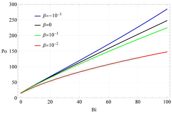
Figure 3.
The Poiseuille number (Po) is shown as a function of the Bingham number (Bi) for different dimensionless values (see Equation (45)) for the Hagen–Poiseuille pipe flow of a single fluid that follows the Parabolic model.
2.3. Hagen–Poiseuille Equation for Non-Newtonian Pipe Flow: Coaxial Flow of Two Immiscible Fluids
The existence of a lubrication layer resulted in a dual-fluid model in which bulk concrete and lubrication fluid with different rheological properties are in contact with each other and flow together, with a distinct interface separating them. This section will introduce the derivation of the flow rate expression for the co-axial pipe flow of dual fluids. The method is essentially the same as that detailed in our recent work [41].
Depending on the type of concrete being pumped, it is possible to have two cases, where either or . For —henceforward referred to as “Case I”—only plug flow is experienced by the bulk concrete. This case is common for the pumping of CVC [34]. For the other case—henceforward referred to as “Case II”—where , two types of flows are experienced by the bulk concrete. In the region of plug flow occurs, while in the region of shear flow occurs. Case II is common for the pumping of SCC [34,36,55,56]. Here, the plug radius is given by
where is the yield stress of bulk concrete.
From Equations (20) and (24), we see that if there is a slip velocity at the wall, let it be , then the flow rate becomes
where depends on the G-parameter (pressure drop per unit pipe length) and the pipe radius R, and shear rate function depends on the rheological properties (denoted by ) of the fluid. Equation (47) shows that when there is a certain slip velocity at the boundary (), the overall flow rate can be found as a sum of the two terms: the flow rate for when the velocity is zero at the wall and an additional term of . The additional term depends only on the cross-sectional area and the velocity at the wall [41].
In the case of the steady co-axial pipe flow of dual fluids, the flow rate from the fluid in the lubrication layer is given by
where the flow velocity at the interface between the bulk concrete and lubrication layer fluid () is denoted as . In order to derive Equation (48), the result from Equation (47) was used. In Case I, when only plug flow is experienced by the bulk concrete, its contribution to the overall volume flow rate can be obtained as [41]
The overall flow rate–pressure drop relation is obtained as [41]
However, in Case II where a sheared-concrete zone is also present in the bulk concrete along with the zone of plug flow near the pipe center, its contribution to the overall volume flow rate is given by [41]
The overall flow rate–pressure drop relation is thus obtained as [41]
The two cases can be unified into one by the use of the Heaviside step function. The result is
where denotes the Heaviside function: for and for .
3. Results and Discussion
Following the analytical derivations from the previous section for both single and dual-fluid cases, it is possible to obtain the relations on the shear rate distribution, the velocity distribution, and the prediction of volume flow rate for the pressure loss per unit pipe length. For the single-fluid case, the input parameters that are necessary to make these predictions include , where a, b, and c are the three parameters in the parabolic fluid model, R is the radius of the pipe, and G represents the pressure loss per unit pipe length. For the co-axial flow of dual fluids (referred to as the bulk concrete and the lubrication layer fluid in the context of concrete pumping), we shall need four more parameters, the thickness of the lubrication layer, ℓ, and three parameters in the parabolic fluid model for the lubrication layer fluid. One can follow the approaches presented by Equations (24) and (53) to derive the expressions to predict the volumetric flow rate for single and dual fluid cases, respectively, depending on the pressure drop per unit pipe length. In this section, we demonstrate the resulting distributions from the parabolic model and analyze the influence of the model’s parameters. We consider some possible values for the a-parameter, b-parameter, and c-parameter with ranges derived by fitting the Parabolic model to the Herschel–Bulkley model explored in our recent work [41].
3.1. Parabolic Model: Shear Stress and Shear Rate Distribution
Figure 4 shows the influence of the -parameter of the bulk concrete for the curves showing the relationship between shear stress and the shear stress using the Parabolic model. Figure 4a shows the shear rate vs. shear stress curve with the influence of this parameter, while Figure 4b presents the conventional approach of shear stress vs. shear rate curves with the shear rate being on the x-axis as the independent variable. From both figures, the effect of varying the -parameter can be clearly observed in how it influences either the shear thickening or the shear thinning behavior of the fluid. With the increase in the analyzed parameter, the shear thinning behavior of the fluid is more prominent for both curves, where there is a more noticeable increase in shear stress with the increase in shear rate. The same is true for the analysis of shear thickening behavior; as with the decrease in the -parameter, the shear stress grows slower with the increase in shear rate. Likewise, for Figure 4b, as the value of the -parameter is increased, the shear rate rises slower and as the parameter is decreased, the curves rise faster with the increasing shear stress corresponding to the shear thinning and shear thickening behavior, respectively. It should be noted that Figure 4b demonstrates that the parabolic model can easily reproduce the shear stress vs. shear rate curve predicted by the Herschel–Bulkley model [41], and the c-parameter of the parabolic model and n-parameter of the Herschel–Bulkley model are similar in nature.
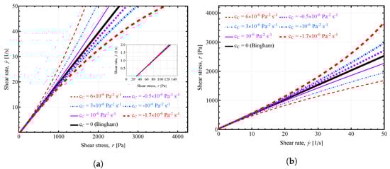
Figure 4.
Influence of -parameter of the bulk concrete: (a) on shear rate vs. shear stress curves predicted by the Parabolic model; (b) on shear stress vs. shear rate curves predicted by the Parabolic model. Unless otherwise specified in the figure, the following values were used: , , , .
In Figure 5, the shear rate vs. shear stress curves are presented with the influence of other parameters from the Parabolic model, Figure 5a showing the effect of varying the -parameter on the curves, and Figure 5b including the effect of varying the -parameter on the shear rate curves. For Figure 5a, it can be observed that the most noticeable effect of varying the -parameter is a change in yield stress values. With the decrease in this parameter, the curves’ x-intercepts shift more to the right, indicating an increase in the values of yield stress. Such results are expected given the expressions for the yield stress derived from the Parabolic model, as presented in Equation (8). In the case of Figure 5a, the -parameter has a more significant influence on the shear rate vs. shear stress curve, unlike the -parameter. This is consistent with previously reported results [36,41,57] because the b-parameter is inversely related to the plastic viscosity derived from the parabolic model when it reduces to the Bingham model as given by Equation (11).
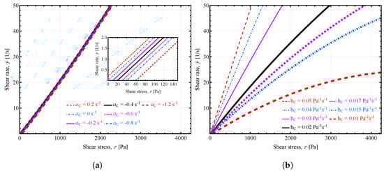
Figure 5.
Shear rate vs. shear stress curves predicted by the Parabolic model: (a) influence of -parameter of the bulk concrete; (b) influence of -parameter of the bulk concrete. Unless otherwise specified in the figure, the following values were used: , , , , .
3.2. Single-Fluid Model
3.2.1. Shear Rate and Velocity Distribution
Figure 6 shows the influence of the -parameter of the bulk concrete on the velocity distribution and shear rate distribution. Figure 6a,b show the shear flow and plug flow regions in the bulk concrete, but plug flow is not visible in the figure due to the small plug radius. This is common for the pumping of SCC [41]. In Figure 6a, as we increase the c-parameter, the velocity increases for the same radial distance and hence the volume flow rate. This is also true for the shear rate distribution shown in Figure 6b. The shear rate value increases with increasing c-parameter value. This is not surprising because increasing the c-parameter decreases the friction value. Thus, as the fluid is more shear-thinning, , the velocity and shear rate distributions are higher, and when the fluid is more shear-thickening, , the corresponding velocity and shear rate values are lower.
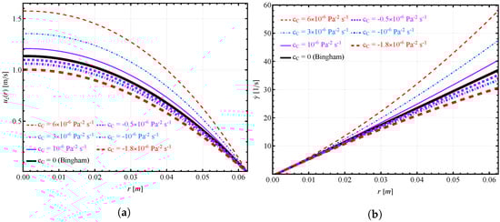
Figure 6.
Influence of -parameter of the bulk concrete: (a) on the velocity distribution; (b) on the shear rate distribution predicted by the Parabolic model. Unless otherwise specified in the figure, the following values were used: , , , , .
3.2.2. Volumetric Flow Rate vs. Pressure Loss
In Figure 7, the volume flow rate relationship is shown: Figure 7a demonstrates how changing the values of the -parameter affects the volume flow rate vs. pressure loss per unit pipe relation for the single fluid flow; Figure 7b presents the influence of the -parameter on the volume flow rate while varying pressure loss per unit pipe length in contour form. Based on Figure 7a, an increase in the value of the -parameter also results in a steeper increase in volume flow rate curves. Similarly to Figure 4b, Figure 7a shows the same influence of the c-parameter of the parabolic model and the n parameter of the Herschel–Bulkley model [41] on the flow rate–pressure drop relation. From Figure 7b, it is clearly seen that, at low values of , the influence of the c-parameter is negligible, but as we increase , its effect becomes predominant. As we increase the c-parameter from low to high, the volume flow rate increases for the same pressure drop. This is expected because, as we increase the c-parameter, the value also increases, resulting in lower friction, as given in Figure 3.
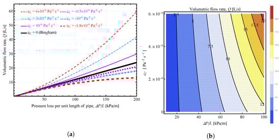
Figure 7.
(a) Influence of -parameter on volume flow rate vs. pressure loss per unit pipe for the single fluid flow predicted by the Parabolic model; (b) contour plot of the volumetric flow rate as a function of the pressure loss per unit pipe length, , as the x-axis and -parameter on the y-axis. Unless otherwise specified in the figure, the following values were used: , , .
3.3. Dual Fluid Model
For the dual fluid case, the rheological properties of both bulk concrete and the lubrication layer of the fluid affect the volume flow rate predictions. Figure 8 shows the volume flow rate vs. pressure loss per unit pipe length for the dual fluid case predicted by the Parabolic model based on Equation (53). Figure 8a presents the influence of the -parameter of the bulk concrete and Figure 8b presents the influence of the -parameter of the lubrication layer of the fluid. Both figures demonstrate the same trend as in Figure 7a, where for smaller values of pressure drop, the influence of the c-parameter on the flow rate is negligible, whereas for bigger values it becomes predominant. Comparing these two figures, it can be seen that both of these parameters have a similar effect on the volume flow rate curves: increasing the c-parameter increases the volume flow rate due to low friction.
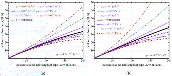
Figure 8.
Volume flow rate vs. pressure loss per unit pipe length for the dual fluid flow predicted by the Parabolic model: (a) influence of -parameter of the bulk concrete with for the fluid in the lubrication layer; (b) influence of -parameter of the fluid in the lubrication layer with for the bulk concrete. Unless otherwise specified in the figure, the following values were used: , , , , , , , .
Similar to Figure 8, Figure 9 presents the influence of the a-parameter on the volume flow rate as a function of pressure loss per unit pipe length for bulk concrete and the lubrication layer of the fluid. Figure 9a shows the effect of the -parameter of the bulk concrete and Figure 9b shows the effect of the -parameter of the lubrication layer of the fluid on the volume flow rate values. Both figures show the same trend that the volume flow rate is not affected by the variation in values of the a-parameter, both for the bulk concrete and the lubrication layer of the fluid. This result is true for the whole range of pressure loss per unit pipe length used in the figures.
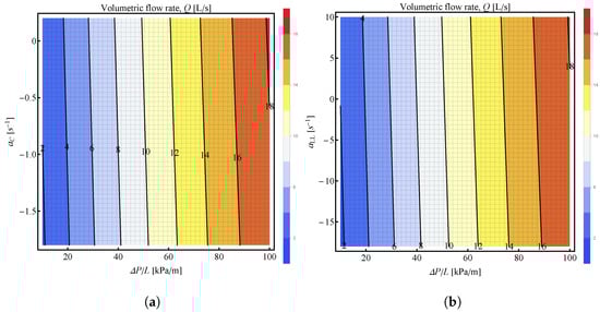
Figure 9.
Contour plots of the volumetric flow rate as a function of the pressure loss per unit pipe length, , as the x-axis and a-parameter on the y-axis: (a) -parameter of the bulk concrete on the y-axis; (b) -parameter of the fluid in the lubrication layer on the y-axis. Unless otherwise specified in the figure, the following values were used: , , , , , , , .
When considering Figure 10, the results are similar to those of Figure 7b. In Figure 10, contour plots for the volumetric flow rate as a function of pressure loss per unit length and b-parameter are presented: Figure 10a shows the influence of the -parameter of the bulk concrete and Figure 10b shows the influence of the -parameter of the lubrication layer of the fluid. In the case of the -parameter of the bulk concrete in Figure 10a, it can be seen that while the effect of varying this parameter is not that prominent for the low values of , it becomes more prominent towards the end of the used range of on the graph. The same is true for the -parameter of the lubrication layer of the fluid, that the influence of the parameter becomes more noticeable with the increase in values of . It can be seen that, at high values of , the larger the and -parameters, the larger the volume flow are under a given pumping pressure. This is not surprising because the larger the b-parameter, the smaller the plastic viscosity of the fluid (Equation (11)), and previously reported studies [41] have shown that for smaller values of and , the volume flow rate is larger for the same pressure drop.
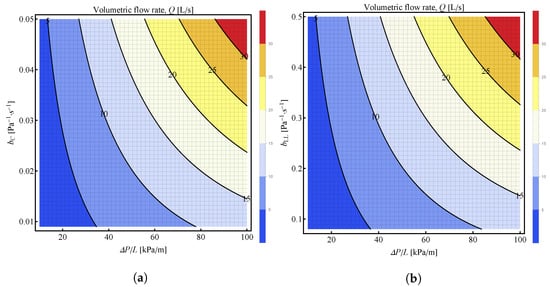
Figure 10.
Contour plots of the volumetric flow rate as a function of the pressure loss per unit pipe length, , as the x-axis and b-parameter on the y-axis: (a) -parameter of the bulk concrete on the y-axis; (b) -parameter of the fluid in the lubrication layer on the y-axis. Unless otherwise specified in the figure, the following values were used: , , , , , , , .
3.4. Computational Apps for the Parabolic Model
Using the analytical expressions derived for the single-fluid and dual-fluid cases and the necessary rheological parameters, one can predict the relationship between the volume flow rate and pressure loss per unit pipe of length. Furthermore, different software and programming languages can be used to easily obtain the necessary curves by inserting the parameters corresponding to the bulk concrete and lubrication layer.
To facilitate applications of our theoretical results in practice, a demonstration application using the Wolfram Mathematica software (version 13.2) has been developed, with a sample graph shown in Figure 11. Users can manipulate the values of the rheological parameters for both bulk concrete and the lubrication layer of the fluid, the diameter of the pipe, and the lubrication layer thickness within the ranges of values written in the program. The resulting graph shows the total volume flow rate vs. the pressure loss per unit pipe length. Furthermore, the application can be used for the analysis purposes of the relation on how the parameters of the bulk fluid, the lubrication layer, the pipe diameter, and the lubrication layer thickness influence the resulting curve.
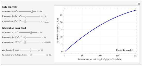
Figure 11.
The graphical user interface of a Wolfram-based demonstration App that presents the volume flow rate vs. pressure loss per unit pipe length curve for the dual-fluid pipe flow of the Parabolic model (See Equation (53)). The following values were used for the computational app in the figure: , , , , , , , .
4. Limitations of the Present Work
In this section, the main assumptions and limitations of the existing work are summarized, along with the future study to be conducted. The main assumptions and limitations are similar to those reported by Kwon et al. [35], Khatib and Khayat [36], and Zhaidarbek et al. [41]. For the analytical derivations, the Hagen–Poiseuille equation is used as the governing law. Therefore, the derived equations are limited to the fully developed, steady, laminar, one-dimensional, and isothermal flow, with the fluids being incompressible, homogeneous, and experiencing no change in their properties during pumping. The rheological properties of the bulk concrete and lubrication layer of the fluid are considered separately and with time independence. The pipe diameter and thickness of the lubrication layer are assumed as constant, and the lubrication layer thickness is also independent of the fluid’s rheological properties. Finally, the difference in the densities of bulk concrete and lubrication layer fluid is considered as negligible.
Despite these limitations, the rheological characteristics of the fluid in the lubricating layer are challenging to estimate experimentally. For the parabolic model, there are four parameters for the lubrication layer fluid: -parameter, -parameter, -parameter, and lubrication layer thickness ℓ, that need to be determined in order to calculate the flow rate–pressure drop relation. One approach to solve this problem is to use a wall-slip model to approximate the dual-fluid flow rate–pressure drop relation. According to the wall-slip model, Equation (53) can be simplified to
where the first term is the single-fluid flow rate in Equation (28) using the bulk concrete parameters and is the additional flow rate that occurs due to the slip effects on the surface. The latter is given by
where is the wall-slip velocity. Using the wall-slip model, the lubrication layer fluid properties can be characterized by just one parameter—the wall-slip velocity. The wall-slip velocity represents a macro-scale description of the wall’s boundary condition [58,59,60,61,62] and depends on the lubrication layer fluid at the wall. This velocity can be estimated in capillary tubes [16]. Consequently, a future goal is to validate the applicability of the wall-slip model in estimating the dual-fluid flow rate–pressure drop relationship in concrete pumping.
5. Conclusions
In this study, rheological models with shear stress as the independent variable are considered, contrasting the conventional approach of using shear rate as the independent variable. The parabolic model is analyzed by dimensional analysis and employed for analytical predictions of the flow rate vs. pressure drop relations in Hagen–Poiseuille pipe flow for a single fluid and in the co-axial flow of dual-fluids. A key advantage of the parabolic model is its ability to account for the nonlinearity of the shear stress and shear rate relations through the inclusion of the nonlinear c-parameter, leading to more accurate results compared to linear models such as the classical Bingham model.
Theoretical derivations have been conducted to derive analytical results for the shear rate distribution, velocity distribution, and volume flow rate relations for Hagen–Poiseuille flow in viscoplastic fluids. This method, which is applied to the parabolic model in this paper, can be generalized for other models with shear stress as the independent variable. This study presents not only the analytical expressions but also explores the effects of the a, b, and c parameters.
While studying the flow curves (i.e., shear rate vs. shear stress curves) for the parabolic model, it is demonstrated how the value of the c-parameter affects the curves: if the value is reduced to , the curve reduces to that of the Bingham model, while a positive c value corresponds to the shear thinning behavior, and a negative c value corresponds to the shear thickening behavior. The b parameter strongly affects the flow curves. In comparison, varying the a-parameter does not have a significant influence on the flow curves.
Subsequently, this study also analyzes the resulting relations based on the parabolic model and how they are influenced by the rheological parameters of the bulk concrete for the single fluid case, along with the lubrication layer for the dual fluid case. For the relation between the volume flow rate vs. pressure loss per unit length of pipe for the single-fluid case, the influence of the c-parameter becomes more prominent for the higher values of pressure drop while being negligible at its low values. For the volume flow rate–pressure drop relation in the dual fluid case, it has been found that varying the a-parameters for both the bulk concrete and lubrication layer fluid has little effect on the relation, while the b-parameters possess a strong effect on the relation with the increasing value of pressure loss per unit pipe length.
Finally, a demonstration App is developed, enabling users to obtain volume flow rate curves by inputting the rheological properties of the bulk concrete and lubrication layer. This application facilitates the study of the influence of rheological parameters on volume flow rate curves and allows for further data analysis.
Supplementary Materials
The following supporting information can be downloaded at: https://www.mdpi.com/article/10.3390/pr11061745/s1, List of Symbols used in the paper.
Author Contributions
B.Z., formal analysis, visualization, software development, writing—original draft; K.S., software development, validation, writing—original draft; Y.W., conceptualization, methodology, supervision, project administration, funding acquisition, writing—review and editing. All authors have read and agreed to the published version of the manuscript.
Funding
The conceptualization of this research originated from a project funded by Nazarbayev University under the Faculty-development competitive research grants program for 2020–2022, Grant №240919FD3925 fdcrgp2019.
Data Availability Statement
The data supporting the findings of this study are available within the article and its Supplementary Materials. The source codes and plotting scripts can be obtained from the corresponding author upon reasonable request.
Acknowledgments
The authors thank Zhumabay Bakenov at the Department of Chemical and Materials Engineering of Nazarbayev University for his valuable input and discussions throughout the course of this research.
Conflicts of Interest
The authors confirm that there are no known competing financial interests or personal relationships that could be perceived as influencing the work presented in this paper.
Abbreviations
The following abbreviations are used in this manuscript:
| CVC | Conventional Vibrated Concrete |
| LL | Lubrication Layer |
| MLT | Mass, Length, and Time |
| ODE | Ordinary Differential Equation |
| SIPM | Shear-Induced Particle Migration |
| SCC | Self-Compacting Concrete or Self-Consolidating Concrete |
References
- Huilgol, R.R.; Georgiou, G.C. Fluid Mechanics of Viscoplasticity; Springer: Cham, Switzerland, 2022. [Google Scholar] [CrossRef]
- Nguyen, Q.; Boger, D. Measuring the flow properties of yield stress fluids. Annu. Rev. Fluid Mech. 1992, 24, 47–88. [Google Scholar] [CrossRef]
- Barnes, H.A. The yield stress—A review or ‘παντα ρει’—everything flows? J. Non-Newton. Fluid Mech. 1999, 81, 133–178. [Google Scholar] [CrossRef]
- Balmforth, N.J.; Frigaard, I.A.; Ovarlez, G. Yielding to stress: Recent developments in viscoplastic fluid mechanics. Annu. Rev. Fluid Mech. 2014, 46, 121–146. [Google Scholar] [CrossRef]
- Coussot, P. Yield stress fluid flows: A review of experimental data. J. Non-Newton. Fluid Mech. 2014, 211, 31–49. [Google Scholar] [CrossRef]
- Bonn, D.; Denn, M.M.; Berthier, L.; Divoux, T.; Manneville, S. Yield stress materials in soft condensed matter. Rev. Mod. Phys. 2017, 89, 035005. [Google Scholar] [CrossRef]
- Bingham, E.C. An Investigation of the Laws of Plastic Flow; Number 278; US Government Printing Office: Washington, DC, USA, 1917. [Google Scholar]
- Bingham, E.C. Fluidity and Plasticity; McGraw-Hill: New York, NY, USA, 1922; Volume 2. [Google Scholar]
- Markovitz, H. Rheology: In the beginning. J. Rheol. 1985, 29, 777–798. [Google Scholar] [CrossRef]
- Mewis, J.; Wagner, N.J. Colloidal Suspension Rheology; Cambridge University Press: Cambridge, UK, 2012. [Google Scholar] [CrossRef]
- Kalyon, D.M. Apparent slip and viscoplasticity of concentrated suspensions. J. Rheol. 2005, 49, 621–640. [Google Scholar] [CrossRef]
- Chhabra, R.P. Non-Newtonian fluids: An introduction. In Rheology of Complex Fluids; Springer: Cham, Switzerland, 2010; pp. 3–34. [Google Scholar]
- Zhou, X.; Li, Z.; Fan, M.; Chen, H. Rheology of semi-solid fresh cement pastes and mortars in orifice extrusion. Cem. Concr. Compos. 2013, 37, 304–311. [Google Scholar] [CrossRef]
- Fernandes, R.; Suleiman, N.; Wilson, D. In-situ measurement of the critical stress of viscoplastic soil layers. J. Food Eng. 2021, 303, 110568. [Google Scholar] [CrossRef]
- Derkach, S.R. Rheology of emulsions. Adv. Colloid Interface Sci. 2009, 151, 1–23. [Google Scholar] [CrossRef]
- Omirbekov, S.; Davarzani, H.; Sabyrbay, B.; Colombano, S.; Ahmadi-Senichault, A. Experimental study of rheological behavior of foam flow in capillary tubes. J. Non-Newton. Fluid Mech. 2022, 302, 104774. [Google Scholar] [CrossRef]
- Vinay, G.; Wachs, A.; Agassant, J.F. Numerical simulation of non-isothermal viscoplastic waxy crude oil flows. J. Non-Newton. Fluid Mech. 2005, 128, 144–162. [Google Scholar] [CrossRef]
- Guedes, R. Viscoplastic analysis of fiber reinforced polymer matrix composites under various loading conditions. Polym. Compos. 2009, 30, 1601–1610. [Google Scholar] [CrossRef]
- Roussel, N.; Coussot, P. “Fifty-cent rheometer” for yield stress measurements: From slump to spreading flow. J. Rheol. 2005, 49, 705–718. [Google Scholar] [CrossRef]
- Roussel, N. Rheology of fresh concrete: From measurements to predictions of casting processes. Mater. Struct. 2007, 40, 1001–1012. [Google Scholar] [CrossRef]
- Roussel, N. (Ed.) Understanding the Rheology of Concrete; Woodhead Publishing Limited: Cambridge, UK, 2012. [Google Scholar]
- Yuan, Q.; Shi, C.; Jiao, D. Rheology of Fresh Cement-Based Materials: Fundamentals, Measurements, and Applications; CRC Press: Boca Raton, FL, USA, 2022. [Google Scholar] [CrossRef]
- De Schutter, G.; Feys, D. Pumping of fresh concrete: Insights and challenges. RILEM Tech. Lett. 2016, 1, 76–80. [Google Scholar] [CrossRef]
- Feys, D.; De Schutter, G.; Fataei, S.; Martys, N.S.; Mechtcherine, V. Pumping of concrete: Understanding a common placement method with lots of challenges. Cem. Concr. Res. 2022, 154, 106720. [Google Scholar] [CrossRef]
- Secrieru, E.; Mohamed, W.; Fataei, S.; Mechtcherine, V. Assessment and prediction of concrete flow and pumping pressure in pipeline. Cem. Concr. Compos. 2020, 107, 103495. [Google Scholar] [CrossRef]
- Choi, M.; Roussel, N.; Kim, Y.; Kim, J. Lubrication layer properties during concrete pumping. Cem. Concr. Res. 2013, 45, 69–78. [Google Scholar] [CrossRef]
- Leighton, D.; Acrivos, A. The shear-induced migration of particles in concentrated suspensions. J. Fluid Mech. 1987, 181, 415–439. [Google Scholar] [CrossRef]
- Phillips, R.J.; Armstrong, R.C.; Brown, R.A.; Graham, A.L.; Abbott, J.R. A constitutive equation for concentrated suspensions that accounts for shear-induced particle migration. Phys. Fluids 1992, 4, 30–40. [Google Scholar] [CrossRef]
- Spangenberg, J.; Roussel, N.; Hattel, J.; Stang, H.; Skocek, J.; Geiker, M. Flow induced particle migration in fresh concrete: Theoretical frame, numerical simulations and experimental results on model fluids. Cem. Concr. Res. 2012, 42, 633–641. [Google Scholar] [CrossRef]
- Choi, M.S.; Kim, Y.J.; Kwon, S.H. Prediction on pipe flow of pumped concrete based on shear-induced particle migration. Cem. Concr. Res. 2013, 52, 216–224. [Google Scholar] [CrossRef]
- Kwon, S.H.; Park, C.K.; Jeong, J.H.; Jo, S.D.; Lee, S.H. Prediction of Concrete Pumping: Part I–Development of New Tribometer for Analysis of Lubricating Layer. ACI Mater. J. 2013, 110, 647–656. [Google Scholar] [CrossRef]
- Secrieru, E.; Khodor, J.; Schröfl, C.; Mechtcherine, V. Formation of lubricating layer and flow type during pumping of cement-based materials. Constr. Build. Mater. 2018, 178, 507–517. [Google Scholar] [CrossRef]
- Kaplan, D. Pompage des Betons. Ph.D. Thesis, Ecole Nationale des Ponts et Chaussées, Paris, France, 1999. [Google Scholar]
- Kaplan, D.; de Larrard, F.; Sedran, T. Design of concrete pumping circuit. ACI Mater. J. 2005, 102, 110. [Google Scholar] [CrossRef]
- Kwon, S.H.; Park, C.K.; Jeong, J.H.; Jo, S.D.; Lee, S.H. Prediction of concrete pumping: Part II-analytical prediction and experimental verification. ACI Mater. J. 2013, 110, 657. [Google Scholar] [CrossRef]
- Khatib, R.; Khayat, K.H. Pumping of Flowable Concrete: Analytical Prediction and Experimental Validation. ACI Mater. J. 2021, 118, 3–16. [Google Scholar] [CrossRef]
- De Larrard, F.; Ferraris, C.F.; Sedran, T. Fresh concrete: A Herschel-Bulkley material. Mater. Struct. 1998, 31, 494–498. [Google Scholar] [CrossRef]
- Feys, D.; Verhoeven, R.; De Schutter, G. Fresh self compacting concrete, a shear thickening material. Cem. Concr. Res. 2008, 38, 920–929. [Google Scholar] [CrossRef]
- Feys, D.; Verhoeven, R.; De Schutter, G. Extension of the Poiseuille formula for shear-thickening materials and application to Self-Compacting Concrete. Appl. Rheol. 2008, 18, 62705. [Google Scholar] [CrossRef]
- Feys, D.; Verhoeven, R.; De Schutter, G. Why is fresh self-compacting concrete shear thickening? Cem. Concr. Res. 2009, 39, 510–523. [Google Scholar] [CrossRef]
- Zhaidarbek, B.; Aruzhan, T.; Galymzhan, B.; Yanwei, W. Analytical predictions of concrete pumping: Extending the Khatib–Khayat model to Herschel-–Bulkley and modified Bingham fluids. Cem. Concr. Res. 2023, 163, 107035. [Google Scholar] [CrossRef]
- Li, M.; Han, J.; Liu, Y.; Yan, P. Integration approach to solve the Couette inverse problem based on nonlinear rheological models in a coaxial cylinder rheometer. J. Rheol. 2019, 63, 55–62. [Google Scholar] [CrossRef]
- Atzeni, C.; Massidda, L.; Sanna, U. Comparison between rheological models for portland cement pastes. Cem. Concr. Res. 1985, 15, 511–519. [Google Scholar] [CrossRef]
- Li, M.; Yan, P.; Han, J.; Guo, L. Which Is an Appropriate Quadratic Rheological Model of Fresh Paste, the Modified Bingham Model or the Parabolic Model? Processes 2022, 10, 2603. [Google Scholar] [CrossRef]
- Matsuhisa, S.; Bird, R.B. Analytical and numerical solutions for laminar flow of the non-Newtonian ellis fluid. AIChE J. 1965, 11, 588–595. [Google Scholar] [CrossRef]
- Meter, D.M.; Bird, R.B. Tube flow of non-Newtonian polymer solutions: PART I. Laminar flow and rheological models. AIChE J. 1964, 10, 878–881. [Google Scholar] [CrossRef]
- Peng, Y.; Ma, K.; Unluer, C.; Li, W.; Li, S.; Shi, J.; Long, G. Method for calculating dynamic yield stress of fresh cement pastes using a coaxial cylinder system. J. Am. Ceram. Soc. 2021, 104, 5557–5570. [Google Scholar] [CrossRef]
- Huilgol, R.R. On the derivation of the symmetric and asymmetric Hele–Shaw flow equations for viscous and viscoplastic fluids using the viscometric fluidity function. J. Non-Newton. Fluid Mech. 2006, 138, 209–213. [Google Scholar] [CrossRef]
- Gerhart, P.M.; Gerhart, A.L.; Hochstein, J.I. Munson, Young and Okiishi’s Fundamentals of Fluid Mechanics; John Wiley & Sons: Hoboken, NJ, USA, 2016. [Google Scholar]
- Bird, R.B.; Stewart, W.E.; Lightfoot, E.N. Transport Phenomena. Revised 2nd ed.; John Wiley & Sons: New York. NY, USA, 2006. [Google Scholar]
- Wang, Y. Steady isothermal flow of a Carreau–Yasuda model fluid in a straight circular tube. J. Non-Newton. Fluid Mech. 2022, 310, 104937. [Google Scholar] [CrossRef]
- Buckingham, E. On plastic flow through capillary tubes. Proc. Am. Soc. Test. Mater. 1921, 21, 1154–1156. [Google Scholar]
- Chhabra, R.P.; Richardson, J.F. Non-Newtonian Flow and Applied Rheology: Engineering Applications, 2nd ed.; Butterworth-Heinemann: Amsterdam, The Netherlands, 2008. [Google Scholar] [CrossRef]
- Morrison, F.A. An Introduction to Fluid Mechanics; Cambridge University Press: New York, NY, USA, 2013. [Google Scholar]
- Feys, D.; De Schutter, G.; Verhoeven, R. Parameters influencing pressure during pumping of self-compacting concrete. Mater. Struct. 2013, 46, 533–555. [Google Scholar] [CrossRef]
- Tavangar, T.; Hosseinpoor, M.; Yahia, A.; Khayat, K.H. Computational Investigation of Concrete Pipe Flow: Critical Review. ACI Mater. J. 2021, 118, 203–215. [Google Scholar] [CrossRef]
- Matthäus, C.; Weger, D.; Kränkel, T.; Carvalho, L.S.; Gehlen, C. Extrusion of lightweight concrete: Rheological investigations. In Rheology and Processing of Construction Materials; Springer: Cham, Switzerland, 2019; pp. 409–416. [Google Scholar]
- Mooney, M. Explicit formulas for slip and fluidity. J. Rheol. 1931, 2, 210–222. [Google Scholar] [CrossRef]
- Oldroyd, J. The interpretation of observed pressure gradients in laminar flow of non-Newtonian liquids through tubes. J. Colloid Sci. 1949, 4, 333–342. [Google Scholar] [CrossRef]
- Jastrzebski, Z.D. Entrance effects and wall effects in an extrusion rheometer during flow of concentrated suspensions. Ind. Eng. Chem. Fundamen. 1967, 6, 445–454. [Google Scholar] [CrossRef]
- Bertola, V.; Bertrand, F.; Tabuteau, H.; Bonn, D.; Coussot, P. Wall slip and yielding in pasty materials. J. Rheol. 2003, 47, 1211–1226. [Google Scholar] [CrossRef]
- Ghahramani, N.; Georgiou, G.C.; Mitsoulis, E.; Hatzikiriakos, S.G. JG Oldroyd’s early ideas leading to the modern understanding of wall slip. J. Non-Newton. Fluid Mech. 2021, 293, 104566. [Google Scholar] [CrossRef]


Disclaimer/Publisher’s Note: The statements, opinions and data contained in all publications are solely those of the individual author(s) and contributor(s) and not of MDPI and/or the editor(s). MDPI and/or the editor(s) disclaim responsibility for any injury to people or property resulting from any ideas, methods, instructions or products referred to in the content. |
© 2023 by the authors. Licensee MDPI, Basel, Switzerland. This article is an open access article distributed under the terms and conditions of the Creative Commons Attribution (CC BY) license (https://creativecommons.org/licenses/by/4.0/).