Article

Batch Process Modeling with Few-Shot Learning

1
State Key Laboratory of Industrial Control Technology, College of Control Science and Engineering, Zhejiang University, Hangzhou 310027, China
2
Department of Chemical Engineering, Chung-Yuan Christian University, Chung-Li District, Taoyuan 320314, China
*
Authors to whom correspondence should be addressed.
Processes 2023, 11(5), 1481; https://doi.org/10.3390/pr11051481
Submission received: 17 March 2023 / Revised: 29 April 2023 / Accepted: 8 May 2023 / Published: 12 May 2023

Abstract

:
Batch processes in the biopharmaceutical and chemical manufacturing industries often develop new products to meet changing market demands. When the dynamic models of these new products are trained, dynamic modeling with limited data for each product can lead to inaccurate results. One solution is to extract useful knowledge from past historical production data that can be applied to the product of a new grade. In this way, the model can be built quickly without having to wait for additional modeling data. In this study, a subspace identification combined common feature learning scheme is proposed to quickly learn a model of a new grade. The proposed modified state-space model contains common and special parameter matrices. Past batch data can be used to train common parameter matrices. Then, the parameters can be directly transferred into a new SID model for a new grade of the product. The new SID model can be quickly well trained even though there is a limited batch of data. The effectiveness of the proposed algorithm is demonstrated in a numerical example and a case of an industrial penicillin process. In these cases, the proposed common feature extraction for the SID learning framework can achieve higher performance in the multi-input and multi-output batch process regression problem.

1. Introduction

The batch process is more flexible than the large-scale continuous production process as the former can better respond to market changes and customer needs. Contrary to the era of big data advocated for in recent years, in many fields, such as chemical process control [1,2] and military electronic product production [3], data are collected with diverse small batch production models employed to cope with rapid product changes [4]. Moreover, the difficulty in collecting data involves many key variables [5], resulting in the problem of small samples in the batch process. Such small samples are called the “low-N problem” [6]. It is difficult to obtain sufficient batches of production data in a certain manufacturing period because of the long operation time, complex operation steps, expensive costs for data collection, and insufficient manpower and material resources. It is not uncommon for the new chemical compounds to run only once or twice in the production equipment, resulting in a low-N scenario in the production of new products [7].
The problem of small samples has been studied in many fields. Some solutions have been used to enhance the robustness of the results obtained from the follow-up training by adding more information to the data or to assist the training of the target by transferring knowledge or data from other aspects [8]. Tulsyan et al. [7] considered using the data sampled repeatedly by hardware to train a GP-based generator and generate a large number of data; then, the authors used the generated data for further process modeling. This method of requiring hardware to repeat sampling may not be implemented in every process; in particular, the measurement data of some key variables are difficult to obtain many times. In addition, the quality of the samples generated by the generator providing auxiliary information is not as good as expected. Zhang et al. [9] combined the physical model and data-driven model, and then a hybrid model framework was proposed to model the process with fewer data in some operating conditions and applied to the dynamic model prediction of algae lutein synthesis. This method is not for practical applications as it is often difficult to obtain the mathematical model in most of the complicated batch processes.
In the industrial batch process, there may be a number of data for other similar products produced in the past. As the current producing product and the past similar product data are measured in the same process, they must share some similar or even the same features. It is reasonable to extract the information from data in these different grades of products that are highly relevant to the current (or target) produced product. Then, the target process model with the transferred data information can be enhanced. Jaeckle et al. [10] proposed extended principal component regression (EPCR), which combines the output data of similar old processes with the output data of the new process for calculation. However, EPCR does not consider the input information of the process, which is unfavorable for a regression problem. Muñoz et al. [11] extended EPCR, considered the input information, and proposed Joint-Y PLS (JY-PLS). In JY-PLS, the variables of the output data are supposed to have the same statistical distributions. Recently, the method based on JY-PLS has been applied to process quality prediction and soft sensing [12,13]. Chu et al. [14] considered the shortage of new data in the initial operation stage of the batch and used the latent variable process migration model (LV-PTM) to transfer similar process data to the new batch of the initial stage. These transfer-based methods require sufficient source data from the same source, which may not be applicable to all kinds of small data scenarios. The above methods based on transfer learning allow the target to transfer knowledge from the data of a single source. However, the data from a single source often does not have enough information as a reliable source of knowledge. The data collected are often diverse, and the number of individual data is small. Therefore, it is necessary to maximize and efficiently use all source data.
Yamaguchi et al. [15] used multi-task learning (MTL) to address the data scarcity of each product in the multi-level batch process. By sharing useful information among multiple related grade products, MTL can improve the accuracy of the model in the case of data shortage. Although MTL makes use of the data of all small sample products for mutual assistance and complementarity, it does not focus on the modeling and analysis of new products. It also does not provide the common information of all collected data. To obtain knowledge transferred from the multiple tasks for the learning of new tasks, Tripuraneni et al. [16] proposed a method to learn common feature representation from multiple tasks, so the data of the new task can be projected into this representation, which can reduce the number of samples required to find the best regressor on the new task. Combining data from multiple products with small samples can help compensate for the limitations of using the data from a single source. However, in the research conducted by Tripuraneni et al. [16], only the common feature space of the input was extracted without considering the dynamic variables. It is impossible to extract shared knowledge of industrial processes in general dynamic MIMO systems.
In this study, a method for batch process modeling with the low-N problem is proposed. The method extracts common features from multi-grade batch process data and incorporates these features into the subspace identification for the new batch process modeling. The problem and novelties considered in this study are summarized as follows:
  • The proposed method considers the characteristics of batch processes, including their multi-input and multi-output structures, their dynamic behavior, and the issue of the uneven length of collected data. The dynamic behavior of the batch process is described using a linear time-invariant state-space (LTI-SS) model, and the original data are used for modeling without the need for data warping.
  • To extract common parts from the historical data, we propose a modified version of the state-space model, which further divides the original model parameters into common and individual parts.
  • When using the proposed model, the input-output equation derived from the proposed LTI-SS model has two coupled common features. We introduce the technique of oblique projection to separate the two parameters so that it can avoid computationally expensive iterative solutions and problems that may not converge.
  • Based on the two separate sets of equations, we derive and organize their final solutions, which can be obtained by calculating the eigenvalue decomposition.
  • Based on the modified state-space model, we combine it with the subspace identification method, and through the substitution of common knowledge, we can effectively improve the modeling performance in the case of a few samples.
The rest of this article is organized as follows. In Section 2, the input-output equation and the problem to be solved are specifically defined. Section 3 introduces the oblique projection to separate the input-output equation into z-space and u-space, respectively. In Section 4, the common feature parameter matrices in the model are estimated by solving the objective function defined in Section 3. In Section 5, the calculated common feature parameter matrices are applied to model the batch data of a new task. Then, the model of the new task can be quickly identified even though there is a small number of batch data in the new task. In Section 6, two examples, including a numerical case and a case of industrial penicillin production, show the performance of the proposed method. In Section 7, the conclusion is given. Finally, to enable readers to quickly and clearly understand the meaning of each symbol, a table is included in Nomenclature; it allows readers to easily compare and refer to it while reading.

2. Problem Formulation and Description

The chemical batch process often exhibits nonlinear and dynamic behaviors. Measurements of process variables are expected to be strongly serially correlated. There are additional characteristics of the long duration and operation in different operating conditions at different phases. To ensure the process is stirred evenly and the reaction is complete, the process is deliberately operated in a fixed operating condition for a while at each operation phase. Thus, the local behavior at each operation phase tends to be linear. To produce different grades of products, the batch process is operated in different operating conditions at different phases, but there are similar behaviors in the physical or chemical properties in each production process [17]. Thus, very limited batch data are often available for each grade of the operating batch, particularly in the new grade produced at the moment of the initial operation period. Only using the limited data of the new batch is certainly insufficient for establishing reliable models, while the model trained by directly extracting knowledge from all grades of batch data has a bias in favor of the graded products with more batch data.
To obtain common knowledge from different grade sources, consider G different types of batch production processes, which are diverse but similar. The dataset D g of the task (the production grade) g is:
D g = ( u g , 1 1 , y g , 1 1 ) ( u g , K g I g I g , y g , K g I g I g )
where I g s ; g = 1 , , G is the number of batches in the production grade g , u g , k i L × 1 and y g , k i M × 1 are the input data and the output data at the k th sampling time of the i th batch data in the production grade g , respectively, i = 1 , , I g ; k = k 0 , k 0 + 1 , , K g i , g = 1 , , G , and K g i is the operation time of the i th batch in the production grade g .
Similarly, for the modeling of new tasks, new batches in the production grade G + 1 are
D G + 1 = u G + 1 , 1 1 , y G + 1 , 1 1 , , u G + 1 , K G + 1 I G + 1 I G + 1 , y G + 1 , K G + 1 I G + 1 I G + 1
To properly describe the dynamic characteristics of the operating batch process, the state-space model is appropriate for multi-input and multi-output dynamic processes. Thus, for the production grade g of the operating batch process, a linear time-invariant state-space model for each phase can be written by:
x g , k + 1 i = A g x k i + B g u g , k i y g , k i = C g x g , k i + ε g , k i
where y g , k i M × 1 and x g , k i N x × 1 are M -dimensional system output and N x -dimensional system states of the i th batch in the production grade g at the sampling time k , respectively. u g , k i L × 1 is the L -dimensional system input of batch i in the production g at the time point k . It is assumed to have Gaussian distribution. ε g , k i M × 1 is an M -dimensional additional noise of batch i in the production grade g at the time point k . It is independent of u g , k i and follows the Gaussian distribution. A g N x × N x , C g M × N x , and B g N x × L are the parameters of batch production grade g . Some common features ( C c and B c ) in the parameters C g and B g are shared in all different grades, expressed as:
C g = C c Q g B g = R g B c
where C c M × N q and B c N r × L have N q orthogonal column vectors and N r orthogonal row vectors, respectively, and Q g N q × N x and R g N r × L are the remaining parts for each grade. With the common features ( C c and B c ), Equation (3) can be rewritten as
x g , k + 1 i = A g x g , k i + R g B c u g , k i y g , k i = C c Q g x g , k i + ε g , k i
Equation (5) is then expressed in the form of the Hankel matrices.
Y g , f i = Γ g , x X g , f i + L g , u U g , f i + E g , f i
where all of the Hankel matrices have a dynamic window size of N , and the number of moving windows is J g i = K g i N :
Y g , f i = y g , N + 1 i y g , N + 2 i y g , N + J g i i y g , N + 2 i y g , N + 3 i y g , N + J g i + 1 i y g , 2 N i y g , 2 N + 1 i y g , 2 N + J g i 1 i N M × J g i
U g , f i = u g , N + 1 i u g , N + 2 i u g , N + J g i i u g , N + 2 i u g , N + 3 i u g , N + J g i + 1 i u g , 2 N i u g , 2 N + 1 i u g , 2 N + J g i 1 i N L × J g i
X g , f i = x g , N + 1 i x g , N + 1 i x g , N + J g i 1 i N x × J g i
E g , f i = ε g , N + 1 i ε g , N + 2 i ε g , N + J g i i ε g , N + 2 i ε g , N + 3 i ε g , N + J g i + 1 i ε g , 2 N i ε g , 2 N + 1 i ε g , 2 N + J g i 1 i N M × J g i
Γ g , x = C c Q g C c Q g A g C c Q g A g N 1 N M × N x
L g , u = 0 0 0 C c Q g R g B c 0 0 C c Q g A g N 2 R g B c C c Q g R g B c 0 N M × N L
As the state term X g , f i of the system is unknown, the past input and output data are used to approximate it:
X g , f i Φ g , z Z g , p i
where
Φ g , z = A g N Γ g , x Δ g A g N Γ g , x L g , u N x × N M + L
Δ g = A g N 1 B g A g N 2 B g B g ;   Z g , p i = Y g , p i U g , p i N M + L × J g i
Y g , p i = y g , 1 i y g , 2 i y g , J g i i y g , 2 i y g , 3 i y g , J g i + 1 i y g , N i y g , N + 1 i y g , N + J g i 1 i ;   U g , p i = u g , 1 i u g , 2 i u g , J g i i u g , 2 i u g , 3 i u g , J g i + 1 i u g , N i u g , N + 1 i u g , N + J g i 1 i
Equation (6) can be further rewritten as:
Y g , f i = Γ g , x Φ g , z Z g , p i + L g , u U g , f i + E g , f i
Now Γ g , x (Equation (11)) and L g , u (Equation (12)) are substituted into Equation (14), expressed as:
Y g , f i = I C c Q g Q g A g Q g A g N 1 Φ g , z Z g , p i + I C c 0 0 0 Q g R g 0 0 Q g A g N 2 R g Q g R g 0 I B c U g , f i + E g , f i
To obtain a more compact expression, some notations shown as follows are defined.
Ω = I N C c N M × N N q Θ = I N B c N N r × N L
O g = Q g Q g A g Q g A g N 1 Φ g , z N N q × N M + L Ξ g = 0 0 0 Q g R g 0 0 Q g A g N 2 R g Q g R g 0 N N q × N N r
Thus, Equation (15) becomes:
Y g , f i = Ω O g Z g , p i + Ω Ξ g Θ U g , f i + E g , f i
Then, each column in Equation (18) can be written as:
y g , f , j i = Ω O g z g , j i + Ω Ξ g Θ u g , f , j i + ε g , f , j i
where Ω and Θ are unknown parameter matrices to be estimated. In this work, an oblique projection, which is used to solve Ω and Θ , is discussed in the next subsection.

3. Model Decomposition into the z-Space and the u-Space Using Oblique Projection

Since Ω and Θ in Equation (18) are coupled together, to avoid solving these two parameters with the iterative way, the technique of oblique projection [18] is applied here to separate Equation (18) into two subspaces which lie in z g , j i and u g , f , j i , respectively. The oblique projection / u g , f , j i z g , j i represents the projection onto z g , j i along the direction parallel to the input vector u g , f , j i .
/ u g , f , j i z g , j i = z g , j i T z g , j i P u , g , j i z g , j i T 1 z g , j i P u , g , j i
where P u , g , j i = I u g , f , j i T u g , f , j i u g , f , j i T u g , f , j i is the projection operator for computing orthogonal complementary spaces of u g , f , j i . With Equations (19) and (20), it is projected along the input matrix u g , f , j i onto z g , j i , expressed as:
y g , f , j i / u g , f , j i z g , j i = Ω O g z g , j i / u g , f , j i z g , j i + Ω Ξ g Θ u g , f , j i / u g , f , j i z g , j i + ε g , f , j i / u g , f , j i z g , j i
According to the assumption of data u g , f , j / u g , f , j i z g , j i = 0 and ε g , f , j i / u g , f , j i z g , j i = 0 . Define the notation φ g , j i = y g , f , j i / u g , f , j i z g , j i ; then, the above equation can be further expressed as:
φ g , j i = Ω O g z g , j i
By combining all of the batch data g = 1 , , G ; i = 1 , , I g ; j = 1 , , J g i , one wants to search for the parameter matrices, O g and Ω . Assume that Ω has the orthogonal structure, and then minimize the sum of squared error defined by:
min Ω , O g Ψ g B Ω O g Z g , p B F 2 s . t .   Ω T Ω = I
where F is the Frobenius norm, and g = 1 , , G .
Ψ g i = [ φ g , 1 i φ g , J g i i ] Z g , p i = [ z g , 1 i z g , J g i i ]
and
Ψ g B = [ Ψ g 1 Ψ g I g ] Z g , p B = [ Z g , p 1 Z g , p I g ]
Equation (23) is called the z-space model.
Similarly, using the oblique projection method, Equation (19) is projected onto u g , f , j i along with the matrix of the past inputs and the outputs z g , j i .
/ z g , j i u g , f , j i = u g , f , j i T u g , f , j i P z , g , j i u g , f , j i T 1 u g , f , j i P z , g , j i
where P z , g , j i = I z g , j i T z g , j i z g , j i T z g , j i is the projection operator for computing orthogonal complementary spaces of z g , j i . With Equations (19) and (26), it is projected along z g , j i onto the input matrix u g , f , j i , and both sides multiplied by Ω T can expressed as:
Ω T y g , f , j i / z g , j i u g , f , j i = O g z g , j i / z g , j i u g , f , j i + Ξ g Θ u g , f , j i / z g , j i u g , f , j i + Ω T ε g , f , j i / z g , j i u g , f , j i
where z g , j i / z g , j i u g , f , j i = 0 , ε g , f , j i / z g , j i u g , f , j i = 0 and u g , f , j i / z g , j i u g , f , j i = u g , f , j i . Define notation λ g , j i = Ω T y g , f , j i / z g , j i u g , f , j i ; then, the above equation can be further expressed as:
λ g , j i = Ξ g Θ u g , f , j i
Similarly, all batch data g = 1 , , G ; i = 1 , , I g ; j = 1 , , J g i are combined. One wants to search for the parameter matrices, Ξ g and Θ . First, assume that Θ has the orthogonal structure; then, minimize the sum of squared errors defined by:
min Θ ,   Ξ g Λ g B Ξ g Θ U g , f B F 2 s . t .   Θ Θ T = I
where
Λ g i = [ λ g , 1 i λ J g i i ] U g , f i = [ u g , f , 1 i u g , f , J g i i ]
and
Λ g B = [ Λ g 1 Λ g I g ] U g , f B = [ U g , f 1 U g , f I g ]
Equation (29) is called the u-space model. Thus, the common parameter matrices ( Ω and Θ ) and the individual parameter matrices ( O g and Ξ g ) of the model defined in Equation (19) can be solved by separately minimizing the two objective functions.

4. Common Feature Parameter Matrices ( Ω and Θ ) Estimation

4.1. Ω and O g Estimation in the z-Space

To solve Equation (23), first consider the loss function for each sub-task parameter, expressed as:
J 1 g = Ψ g B Ω O g Z g , p B F 2
Taking Equation (32) derivative with respect to (w.r.t.) each O g ; g = 1 , , G is:
J 1 g O g = 0 = 2 Ω T Ψ g B Z g , p B T 2 O g Z g , p B Z g , p B T
Then, the solution to O g ; g = 1 , , G is directly given.
O g = Ω T Ψ g B Z g , p B T Z g , p B Z g , p B T 1
With the expression of the optimal model parameter O g , Equation (34) is substituted into the loss function (Equation (32)); then, the optimization problem for the common feature parameter Ω becomes:
min Ω Ψ g B Ω Ω T Ψ g B Z g , p B T Z g , p B Z g , p B T 1 Z g , p B F 2 s . t .   Ω T Ω = I
According to the definition of the Frobenius norm, Equation (35) can be expanded as:
g = 1 G Ψ g B Ω Ω T Ψ g B Z g , p B T Z g , p B Z g , p B T 1 Z g , p B F 2 = g = 1 G t r Ψ g B T Ψ g B t r Ω T Ψ g B Z g , p B T Z g , p B Z g , p B T 1 Z g , p B Ψ g B T Ω
Considering the part related to Ω , the objective function (36) can be transformed to:
max Ω g = 1 G t r Ω T Ψ g B Z g , p B T Z g , p B Z g , p B T 1 Z g , p B Ψ g B T Ω s . t .   Ω T Ω = I
The gradient of the objective function at the optimum must be zero. Then, Equation (36) can be written as:
Ψ MT - L Ω = α Ω
where α is Lagrange multiplier, and
Ψ MT - L = g = 1 G Ψ g B Z g , p B T Z g , p B Z g , p B T 1 Z g , p B Ψ g B T
Compute the eigen-decomposition of Ψ MT - L , and let Ω consist of the N q eigenvectors of Ψ MT - L that have the largest N q eigenvalues. Once Ω is obtained, O g can be directly calculated in Equation (34).

4.2. Θ and Ξ g Estimation in the u-Space

Similar to the procedure for solving Equation (29), consider the loss function for each sub-task parameter:
J 2 g = Λ g B Ξ g Θ U g , f B F 2
where g = 1 , , G . By taking Equation (40) derivative w.r.t. each Ξ g and setting it equal to zero, one can obtain:
J 2 g Ξ g = 0 = 2 Λ g B U g , f B T Θ T 2 Ξ g Θ Λ g B Λ g B T Θ T
Then, the solution to Ξ g ; g = 1 , , G is directly given.
Ξ g = Λ g B U g , f B T Θ T Θ U g , f B U g , f B T Θ T 1
With the expression of the optimal model parameter matrix Ξ g , Equation (42) is substituted into the objective function (Equation (29)); then, the optimization problem for the common feature parameter Θ becomes:
min Θ g = 1 G Λ g B Λ g B U g , f B T Θ T Θ U g , f B U g , f B T Θ T 1 Θ U g , f B F 2 s . t .   Θ Θ T = I
With the definition of the Frobenius norm, the loss function in Equation (43) can be expanded as:
g = 1 G Λ g q Λ g B U g , f B T Θ T Θ U g , f B U g , f B T Θ T 1 Θ U g , f B F 2 = g = 1 G t r Λ g B T Λ g B t r Λ g B T Λ g B U g , f B T Θ T Θ U g , f B U g , f B T Θ T 1 Θ U g , f B
Considering the part related to Θ , the objective function (43) can be transformed to:
max Θ g = 1 G t r Θ U g , f B Λ g B T Λ g B U g , f B T Θ T Θ U g , f B U g , f B T Θ T s . t .   Θ Θ T = I
Solving Equation (44) is a nonlinear optimization problem. To reduce the complexity of nonlinear calculation, Θ = θ 1 θ N N r T is calculated row by row. First, take the first-row vector θ 1 of Θ in Equation (45) and make it a derivative w.r.t. θ 1 , which is expressed by:
2 g = 1 G B g θ 1 θ 1 T W g θ 1 θ 1 T B g θ 1 W g θ 1 θ 1 T W g θ 1 2 = 2 β 1 θ 1
where B g = U g , f B Λ g B T Λ g B U g , f B T , W g = U g , f B U g , f B T ; g = 1 , , G . Let ϕ W g , 1 = θ 1 T W g θ 1 , and ϕ B g , 1 = θ 1 T B g θ 1 . Equation (46) can be compactly expressed as
E θ 1 θ 1 = β 1 θ 1
where
E θ 1 = g = 1 G B g ϕ W g , 1 ϕ B g , 1 W g ϕ W g , 1 2
Equation (47) is a nonlinear eigenvalue problem associated with the extracted eigenvector. For this problem, an iterative algorithm can be used [19]. In the first iteration, with the guessed θ 1 0 , the left-hand side of Equation (47) can be computed and an approximation to the eigenvector θ 1 1 associated with the smallest eigenvalue of E θ 1 0 can be estimated. Then, the left-hand side of Equation (47) with the new computed θ 1 1 is updated, and the updated eigenvector θ 1 2 associated with the smallest eigenvalue of E θ 1 1 can be estimated. The above same procedure is repeated until θ 1 1 has no significant change. Once the optimal result θ ^ 1 is found, the deflation technique is used to remove the support and the query sets related to the direction θ ^ 1 :
U g , f 2 = U g , f 1 θ ^ 1 θ ^ 1 T θ ^ 1 1 θ ^ 1 T U g , f 1
Then, the second parameter vector of θ 1 is solved based on Equation (47). The above procedure is repeated until the desired number of vectors is obtained. The whole iterative procedure originated is applied to solving Equation (47) as shown in Algorithm 1.
Algorithm 1: Iterative procedure for the of the parameter Θ estimation.
Input:
B g 0 , W g 0 for g = 1 , 2 , , G and θ i 0
Process:
  • For i = 1 , , N N r
    (1)
    For t = 1 , , until convergence do
    Compute the eigenvalue decomposition of E t θ i t 1 and select the eigenvector to the largest eigenvalues θ i t
    End for
    (2)
    U g , f i = U g , f i 1 θ ^ i θ ^ i T θ ^ i 1 θ ^ i T U g , f i 1
    (3)
    Update B g i and W g i by using U g , f i
    End for
Output:
Θ ^ = θ ^ 1 T θ ^ N N r T
For clarity, the entire procedure for estimating the parameter matrices ( Ω , Θ ) of the model is summarized as shown in Algorithm 2.
Algorithm 2: Algorithm for the estimation of the common features Θ and Ω .
Input:
The normalized set data, u g i L × 1 ,   y g i M × 1 ;   i = 1 , , I g ;   g = 1 , , G
The dynamic step size N
The common feature parameter sizes N q and N r
Process:
  • Arrange the input and output data of each batch of all the products into the Hankel matrix according to equation (18)
  • Using oblique projections equation (20) and (26), get φ g , j i and λ g , j i
  • According to equation (38), calculate the SVD decomposition of Ψ MT - L and take the first N N q eigenvectors to obtain the common parameter matrix Ω
  • Substitute the estimated Ω from into equation (28), and then calculate Θ according to Algorithm1.
Output:
 The common feature parameters Ω and Θ

5. Refining Parameter Matrices Using Testing Sets

Subspace Identification with the Common Feature Parameter Matrices

Once the common feature parameter matrices Ω ^ and Θ ^ are estimated using the meta-training sets, the pre-trained model structure and the corresponding parameter matrices will be transferred to the new batch G + 1 . Then, the new batch with limited batch data can be quickly learned. Substituting Ω ^ and Θ ^ into Equation (18), the input-output matrix equation of the i th batch process is:
Y f i = Ω O ˜ Ω T Y p i + Ω Ξ ˜ Θ U p i + Ω Ξ Θ U f i + E f i
where the batch grade index is omitted as the new batch G + 1 has only one grade.
O ˜ = Q Q A Q A N 1 A N Q Q A Q A N 1 Q Q A Q A N 1 A N 1 R A N 2 R R A N Q Q A Q A N 1 Ξ
Z ˜ p i = Ω T Y p i Θ U p i
The first three terms of the right-hand side of Equation (50) are combined
Y ˜ f i = P W ˜ Z U i + E ˜ f i
where Y ˜ f i = Ω ^ T Y f i , P = O Ξ , E ˜ f i = Ω ^ T E f i , U ˜ f i = Θ ^ U f i , and W ˜ Z U i = Z p i U ˜ f i .
For the solution of Equation (53), the sub-blocks ( Y ˜ f i and W ˜ Z U i ) of all I batches horizontally concatenate as follows:
Y ˜ B = Y ˜ f 1 Y ˜ f I W ˜ Z U , B = W ˜ Z U 1 W ˜ Z U I
Then, the objective function is written as:
min P Y ˜ B P W ˜ Z U , B 2 2
The solution to Equation (55) can be obtained using the least-squares method, and P ^ can be solved uniquely.
P ^ = Y ˜ B W ˜ Z U , B T W ˜ Z U , B W ˜ Z U , B T 1
To further obtain the state-space model parameters, the estimated parameter P ^ is divided into the corresponding matrix:
P ^ = O ^ Ξ ^
According to Equations (6) and (18), Ω T Γ x X f = O Z p . Decompose O ^ Z p with SVD:
O ^ Z p = U 1 U 2 1 0 0 2 V 1 T V 2 T
where 1 is the dominant singular value. The observability matrix and the state sequence of the system can be directly determined from the above SVD:
Γ x Ω = Ω ^ T Γ x = U 1 1 1 / 2 = Q ^ Q ^ A ^ Q ^ A ^ N 1
X ^ f = 1 1 / 2 V 1 T = x ^ N + 1 x ^ J
According to the definition of Γ x Ω , the parameter matrix ( A ^ ) in the new batch production is:
A ^ = Γ x Ω N x + 1 : e n d , : Γ x Ω 1 : e n d N x , :
According to the model in Equation (3), the estimated results X ^ f and A ^ are substituted to obtain:
x ^ N + 2 x ^ J A ^ x ^ N + 1 x ^ J 1 = B u N + 1 u J 1
y N + 1 y J = C x ^ N + 1 x ^ J + ε N + 1 ε J
In addition, the parameter matrices B and C in Equations (61) and (62) can be obtained using the least-squares method.

6. Case Study

Two cases were used to verify the proposed MT-L SID: a numerical example and an industrial penicillin batch production process.

6.1. Numerical Example

Consider a batch system whose model generates input and output data according to Equation (5). Each stage of batch production is regarded as a task ( g ). The input and output numbers are L = 20 and M = 20 , respectively. The order of the system state is N x = 4 . The input of the system ( u g , k i ) is random samples generated from the Gaussian distribution N 0 , 2 I L , and the noise of the system is ε g , k i ~ N 0 , 0.1 I M . The parameter matrices C c M × N q and B c N r × L with N q = 3 and N r = 3 shared in all batches are randomly generated through the Gaussian distribution and orthogonalized. The parameters, A g , R g , and Q g vary with different tasks (batch grades). They are randomly generated with the Gaussian distributions N 0 , 0.2 , N 0 , 1.9 , and N 0 , 2.8 , respectively. The initial state of each grade of the batch g is x g , k i = 0 N x . Assume that there are G different batch grades in the training phase. The data generation of the new batch grade G + 1 is still based on the same above assumptions of model parameter matrices.
To verify the proposed common feature extraction scheme for identifying the subspace model, four cases are demonstrated, including (1) a varying number of grades, (2) a varying number of data in each batch grade, (3) identifying the subspace model for a new grade, and (4) modeling performance with the different common feature parameters N q and N r . The LF-MoM method in [16] was adapted to calculate Equation (28), and the results were used to compare the proposed methods. The principal angle was used to evaluate the difference between the estimated common feature parameter and the actual one. The concept of principal angles between subspaces was first introduced by [20]. Then, Hotelling and Harold [21] defined the form of the canonical relationship of principal angles in the statistical theory. In this paper, the calculation method of the principal angle is based on singular value decomposition (SVD) [22,23].
When using the proposed method to extract common knowledge, the adjustable input parameters are listed in Algorithm 2, including the dynamic window size, N , and the dimensions N q and N r of the two common parameters.
The selection of parameter N is used to extract dynamic features of the process, which theoretically must be greater than or equal to the potential state order N x of the model. In the case of N N x , the performance of the identification will not significantly improve and may even decrease. The larger N is, the more parameters must be calculated, and a higher data volume is required. In the case of fewer samples, the modeling performance will decrease. On the other hand, in the case of N < N x , it cannot adequately reflect the dynamic characteristics of the process, and the resulting model cannot effectively describe the process behavior. Therefore, it is necessary to adjust N appropriately when identifying batch processes with a few samples:
(1)
Varying numbers of grades
Assume that each grade has only two batch data for the common feature extraction stage. Take the number of samples K g = 62 in each training batch. The batch indicator is omitted in this case. The input and output Hankel matrices Y f , U f , and Z p are arranged by taking N = 6 and J g = 50 ( J g = K g N ) from the training data. Then, Ψ g and Λ g are obtained by the oblique projection.
With different grade numbers, G , the common feature parameter matrices ( Ω ^ and Θ ^ ) were estimated. The sine values of the principal angles between the estimated common feature parameter matrices and the actual common feature parameter matrices are shown in Figure 1. The x-axis in Figure 1 is the number of tasks used in the common feature extraction stage, and the y-axis is the sine value of the principal angle sin θ between the actual and the estimated common feature parameter matrices. The smaller sin θ is, the closer the estimated and the actual parameter matrices are. The common characteristic parameters of output variables were not discussed in [17], so only the MT-L SID test results are available. The results show that the accuracy of the parameter matrix Ω ^ can be achieved with fewer data. In the estimation of the parameter matrix Θ ^ , both the results of MT-L SID and LF-MoM are to be improved and need more training grades than the estimated parameter matrix Ω ^ , as the former is for the transmitter model, while the latter is for the emission model. More training grades are to be included for estimating a good parameter matrix Θ ^ . Furthermore, the results show that MT-L SID can achieve a slightly better performance than LF-MoM.
(2)
Varying numbers of data in each batch grade
In the second case, the number of grades was fixed at G = 30 , but different numbers of training samples were applied. With the different samples in each batch, the corresponding dynamic windows J g of the Hankel matrix were changed from 31 to 500, but the window size remained at N = 6 . The principal angles between the estimated common feature parameter matrices and the actual common feature parameter matrices are shown in Figure 2. The x-axis of Figure 2 represents the number of dynamic windows contained in each training batch, and the y-axis is the sine value of the principal angle sin θ between actual and estimated common feature parameter matrices. Similar to Case 1, the parameter matrix Ω ^ with fewer data samples still can provide a good model performance. At the same grade number, increasing the number of dynamic windows can improve the accuracy of the parameter matrix Θ ^ to a certain extent. In addition, Θ ^ estimated from MT-L SID showed better accuracy than LF-MoM.
(3)
System identification of a new grade
A new grade of the product was produced through a single batch. The system model of the new grade was then identified. The new grade in the testing stage had one batch for training and one for testing. The data of one new batch were arranged into the Hankel matrix with N = 6 . With the common feature parameter matrices Ω ^ and Θ ^ obtained with 500 tasks and J = 50 , the model parameter matrices O ^ and Ξ ^ were identified by Equation (56); the corresponding parameter matrices ( A ^ , B ^ , and C ^ ) of the state-space model can be calculated using Equations (57)–(60).
Three models, including the conventional subspace identification (SID), the SID combining the common feature parameters estimated from MT-L SID, and the SID from LF-MoM were, respectively, used for comparisons. Figure 3 shows the poles of the estimated batch parameter matrix A ^ with different numbers of samples for the three models. The black asterisk and the blue, cyan, and red circles represent the actual model, SID, MT-L SID, and SID with common feature parameters estimated from LF-MoM, respectively. In Figure 3a, when the data are insufficient ( J G + 1 = 25 ), the proposed MT-L SID outperformed other models. With the increasing number of training samples, all models were very close to the actual ones in Figure 3b with J G + 1 = 40 and in Figure 3c with J G + 1 = 100 . As for all the case studies, the proposed learning scheme can significantly reduce the training sample requirements in each grade compared to the other modeling schemes.
In the testing stage, the demand for training data can be reduced by including common feature parameter matrices when the target batch data are insufficient. If the target batch data collected in the test phase are already sufficient, then the model directly using only the target batch data without common feature parameters can achieve accurate estimated parameters or better. In this case, adding the common feature parameters for estimation becomes unnecessary. However, at the stage of modeling a new batch process, the proposed learning scheme plays an important role.
  • Modeling performance with the different common feature parameters N q and N r
In the fourth case, quantity and batch grade data were considered to compare the support of selecting different common parameter structures in modeling new grades. Assume there are 100 grades of data, each with two batches of data, and each batch has an operating time of K g = 62 . In terms of parameter settings, take N = 6 ; J g = 50 . Consider the case where N q and N r have different dimensions. Substitute the calculated common feature parameters into the modeling of new product grade data, and further calculate the MSE from the trained model parameters on the test data as an indicator to measure the transfer performance. The calculated results are shown in Table 1.
From Table 1, it can be seen that the best modeling performance can be achieved when the dimensions of the common parameters are the same as the real dimensions. The dimensions N q and N r of the common parameters determine the amount of information transferred from historical data to new batch product modeling. If the selected dimension is greater than the potential actual dimension, then there is still information that can be transferred but not used. If it is smaller than the potential actual dimension, then it will compress the size of the structure describing individual parameters, so the description of the process in system identification is probably under-fitting. Therefore, similarly, the dimensions of common parameters also require several attempts to choose a more appropriate size.

6.2. Industrial Process for Penicillin Fermentation

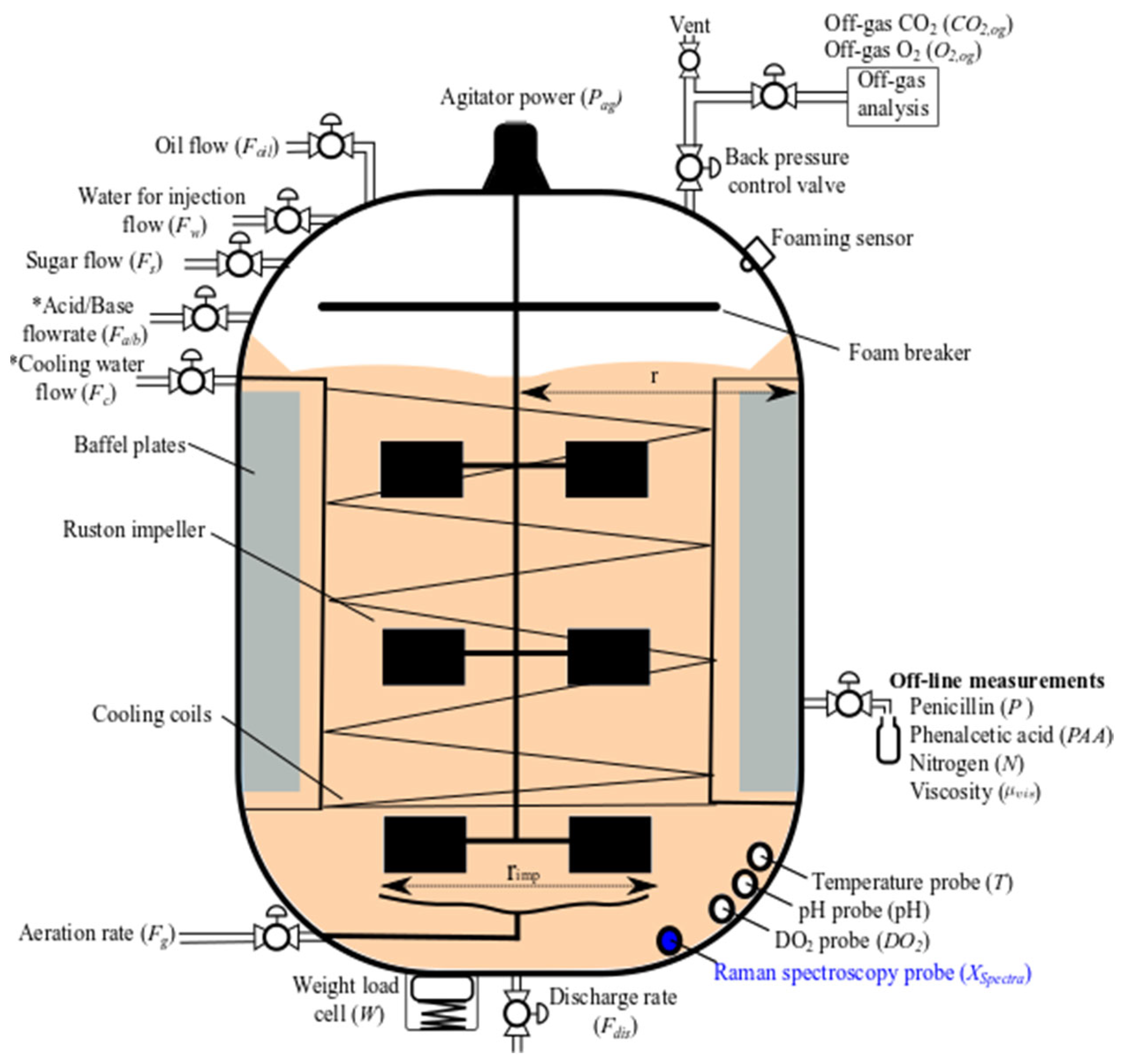
A simulation of industrial-scale penicillin (IndPen) production performed by the authors of [24] was used here to validate the proposed method. The simulation was developed using the historical batch records of a 100,000 L penicillin fermentation using a high-yielding industrial strain of Penicillium chrysogenum, and all the available process inputs and outputs were accurately simulated. At the same time, IndPen also integrated real Raman spectroscopy equipment. In addition to modeling all required online and offline variables, IndPen also considered the growth, morphology, metabolites, and degradation of Penicillium chrysogenum fermentation on a large scale. The process flow sheet from [24] is shown in Figure 4. Further details of the model can be found in [24,25].
The input variables and online collected output variables of the fed-batch penicillin process are listed in Table 2. In the penicillin production process, the sampling time of the variable was 24 min. The variables were divided into two parts for control, namely automatic control variables and manual control variables. The temperature and pH were controlled by automatic control variables and regulated by a proportional integral differential (PID) feedback loop. In the manual control variables, the substrate flow rate and the phenylacetic acid flow rate were controlled by the recipe-driven method following the fixed curve of the whole batch or by the operator operating the fixed curve of the whole batch (depending on the operator). This control mode copied the control actions observed by the operator manually adjusting the whole batch of the substrate flow rate and the phenylacetic acid flow rate.
In IndPen, the operation mode was adjusted as follows.
  • Changing environment temperature.
  • Control strategy (recipe-driven (i.e., SBC)).
  • Option to include inhibitory effects on the growth rates during DO2, N, and PAA limitation, as well as during excessive PAA and CO2 concentrations and sub-optimal T and pH operation.
  • Whether to use Raman spectroscopy to control PAA.
According to the selection of the above modes, 14 different modes were collected. The first 10 modes were operated in ambient temperature condition 1: substrate feed temperature 288 K, substrate feed cold water 288 K, air temperature 290 K, and inlet coolant temperature 285 K. The operation mode setting under these temperature conditions is shown in Table 3. The operation mode setting under temperature condition 2—substrate feed temperature 293 K, substrate supply cold water 293 K, air temperature 298 K, and inlet coolant temperature 288 K—is shown in Table 3.
According to the variables in Table 2, the input and output profiles of mode 1 are shown in Figure 5 and Figure 6, respectively.
In the case of a small sample of batch data, operation mode 10 was selected for validation. The common knowledge was extracted from the data of other modes excluding the test. The proposed MT-L SID was compared with the combination of LF-MoM and SID and the conventional SID.
  • Few-shot learning in mode 10 data
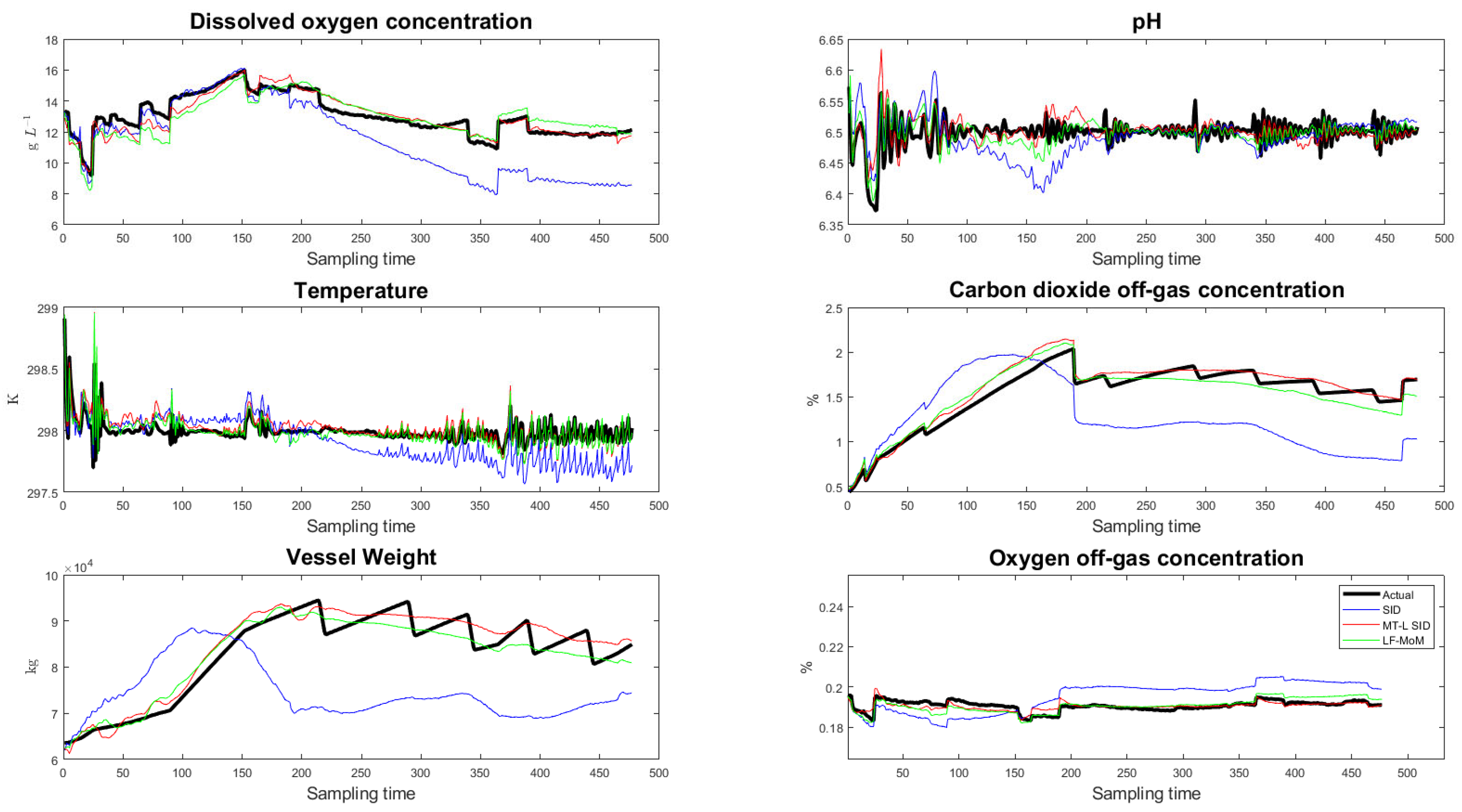
Considering the modeling of fed-batch penicillin process in operation mode 10, the common feature extraction involved using the batch data in other modes, and each of them was five batches. The dimensions of the common feature parameter matrices with N = 36 were N r = 5 and N q = 5 . In the testing stage, nine batch data from mode 10 were used for training, and the rest of the batch was used for verification. The results are shown in Figure 7.
In Figure 7, the black lines are the actual outputs, the blue lines are the predicted outputs without using common feature parameter matrices for modeling, the red lines are the predicted outputs of the MT-L SID, and the green lines are the predicted outputs of the model with LF-MoM. Although the outputs of the red lines do not completely follow the outputs well, the proposed learning model can better describe the process behaviors than the model established without using common feature parameter matrices and SID with LF-MoM. The MSE of these methods with five operation conditions (modes) are shown in Table 4. In Table 4, the process variables are scaled to the same size. The results show that in few-shot batch modeling, the performance of the proposed MT-L SID was helpful and better than LF-MoM and conventional SID.

7. Conclusions

The data collected from the industrial batch process sometimes encounter the low-N problem. Such a small number of batch-run data will greatly degrade the performance of data-driven models. In this study, multitask-learning SID was proposed for modeling batch processes, which can transfer knowledge from multiple batch process data. The proposed method uses historical batch data with similar multiple batch production to train the state-space model and extract common feature parameter matrices. Then, during modeling, a batch with a new grade, as well as the input and output variables of the historical batch data, is projected into the common feature space to reduce the sample requirements for the training of new model parameters. Thus, the model of a new batch with a few batch data can be effectively and quickly constructed. In addition, the purpose of using oblique projection in our method is to avoid solving the common parameters of two objective functions simultaneously during the solution process. This technique can decouple the two parameters so that the solutions of the two parameters do not affect each other. According to the objective functions we have defined, the derivation result of solving the common parameters corresponds to solving the eigenvalue problem. The common parameters correspond to the maximum eigenvalue of the data matrix after the oblique projection transformation. The contributions of this study are summarized as follows:
  • A modified linear time-invariant state-space model was proposed, which separates the common features and individual features corresponding to the input and input parameters so that it can be used to express the extraction of common features in the multi-input, multi-output dynamic system.
  • The multi-task learning-based N4SID, called MT-L SID, was developed. The proposed SID model of the common feature parameters was learned from historical batch data. It can be effectively applied to the batch process with new grades. Then, the data requirement of a new batch process modeling can be reduced.
  • With the oblique projection, MT-L SID can separate input-output equations to calculate the common feature parameter matrices. The calculations are straightforward without heavy iterations.
Finally, the proposed method was validated based on a numerical example and an industrial penicillin production process. In the generated numerical examples, increasing the number of batches (tasks) or the amount of data in individual batches improved the accuracy of common feature parameters. In the production of penicillin, the proposed method showed better prediction performance in the case of a few samples.

Author Contributions

Conceptualization, S.G., J.C. and L.X.; formal analysis, S.G. and J.C.; investigation, S.G., J.C. and L.X.; methodology, S.G. and J.C.; resources, S.G. and J.C.; software, S.G.; supervision, S.G., J.C. and L.X.; visualization, S.G.; writing—original draft, S.G. and J.C.; writing—review and editing, S.G. and J.C. All authors have read and agreed to the published version of the manuscript.

Funding

This research was funded by the Ministry of Science and Technology, Taiwan (MOST 109-2221-E-033-060-MY3), and National Natural Science Foundation of P.R. China (62073286).

Data Availability Statement

Data are available upon request due to restrictions privacy. The data presented in this study are available upon request from the corresponding author.

Conflicts of Interest

The authors declare no conflict of interest.

Nomenclature

D g The data set of batch grade g
I g Number of batches in grade g
N Dynamic window size
x g , k i System state
of batch i in grade g at time k
u g , k i System input
of batch i in grade g at time k
y g , k i System output
of batch i in grade g at time k
ε g , k i Additional noise
of batch i in grade g at time k
B g Parameter of grade g
R g Individual part of parameter B g
C c Common part of parameter C g
B c Common part of parameter B g
Ω Extended of parameter C c
λ g , j i y g , f , j i projection onto u g , f , j i along the direction parallel to z g , j i
Ψ g B Total batch data of φ g , j i
Λ g B Total batch data of λ g , j i
G Number of grades
K g i Operation time of batch i in grade g
J g i Number of moving windows
N x Number of system states
L Number of system inputs
M Number of system outputs
A g Parameter of grade g
C g Parameter of grade g
Q g Individual part of parameter C g
N q Dimention of parameter C c
N r Dimention of parameter B c
Θ Extended of parameter B c
φ g , j i y g , f , j i projection onto z g , j i along the direction parallel to u g , f , j i
Z g , p B Total batch of z g , j i
U g , f B Total batch of u g , f , j i

References

  1. Song, H.; Xu, R.; Wang, C. Research on statistical process control method for multi-variety and small batch production mode. In Proceedings of the 2020 Chinese Control And Decision Conference (CCDC), Hefei, China, 22–24 August 2020; pp. 2377–2381. [Google Scholar]
  2. Wang, J.; Zhang, T.; Wang, C.; Shi, X. Optimizing the Uncertainty of PPM on Small Batch of Quality Data. In Proceedings of the 2021 IEEE 6th International Conference on Smart Cloud (SmartCloud), Newark, NJ, USA, 6–8 November 2021; pp. 107–110. [Google Scholar]
  3. Cao, Y.; Feng, Z.; Jiang, Q. Automatic Data Acquisition Technology for SMT Manufacturing Based on Multi-Variety and Small-Batch. In Proceedings of the Seventh Asia International Symposium on Mechatronics; Springer: Berlin/Heidelberg, Germany, 2020; pp. 528–537. [Google Scholar] [CrossRef]
  4. Li, Q.; Wei, F.; Zhou, S. Early warning systems for multi-variety and small batch manufacturing based on active learning. J. Intell. Fuzzy Syst. 2017, 33, 2945–2952. [Google Scholar] [CrossRef]
  5. Cui, L.; Peng, Y.; Ding, L.; Lu, D. An improved batch fluidized drying experimental design based on digital sensors and a minicomputer. Eng. Rep. 2021, 3, e12366. [Google Scholar] [CrossRef]
  6. Tulsyan, A.; Garvin, C.; Ündey, C. Advances in industrial biopharmaceutical batch process monitoring: Machine-learning methods for small data problems. Biotechnol. Bioeng. 2018, 115, 1915–1924. [Google Scholar] [CrossRef] [PubMed]
  7. Tulsyan, A.; Garvin, C.; Undey, C. Industrial batch process monitoring with limited data. J. Process Control 2019, 77, 114–133. [Google Scholar] [CrossRef]
  8. Weiss, K.; Khoshgoftaar, T.M.; Wang, D. A survey of transfer learning. J. Big Data 2016, 3, 9. [Google Scholar] [CrossRef]
  9. Zhang, D.; Del Rio-Chanona, E.A.; Petsagkourakis, P.; Wagner, J. Hybrid physics-based and data-driven modeling for bioprocess online simulation and optimization. Biotechnol. Bioeng. 2019, 116, 2919–2930. [Google Scholar] [CrossRef] [PubMed]
  10. Jaeckle, C.M.; MacGregor, J.F. Product transfer between plants using historical process data. AIChE J. 2000, 46, 1989–1997. [Google Scholar] [CrossRef]
  11. Muñoz, S.G.; MacGregor, J.F.; Kourti, T. Product transfer between sites using Joint-Y PLS. Chemom. Intell. Lab. Syst. 2005, 79, 101–114. [Google Scholar] [CrossRef]
  12. Rudnitskaya, A.; Costa, A.M.S.; Delgadillo, I. Calibration update strategies for an array of potentiometric chemical sensors. Sens. Actuators B Chem. 2017, 238, 1181–1189. [Google Scholar] [CrossRef]
  13. Jia, R.; Zhang, S.; You, F. Transfer learning for end-product quality prediction of batch processes using domain-adaption joint-Y PLS. Comput. Chem. Eng. 2020, 140, 106943. [Google Scholar] [CrossRef]
  14. Chu, F.; Zhao, X.; Yao, Y.; Chen, T.; Wang, F. Transfer learning for batch process optimal control using LV-PTM and adaptive control strategy. J. Process Control 2019, 81, 197–208. [Google Scholar] [CrossRef]
  15. Yamaguchi, T.; Yamashita, Y. Quality prediction for multi-grade batch process using sparse flexible clustered multi-task learning. Comput. Chem. Eng. 2021, 150, 107320. [Google Scholar] [CrossRef]
  16. Tripuraneni, N.; Jin, C.; Jordan, M. Provable meta-learning of linear representations. In Proceedings of the International Conference on Machine Learning, Vienna, Austria, 18–24 July 2021; pp. 10434–10443. [Google Scholar]
  17. Lu, J.; Yao, K.; Gao, F. Process similarity and developing new process models through migration. AIChE J. 2009, 55, 2318–2328. [Google Scholar] [CrossRef]
  18. Behrens, R.T.; Scharf, L.L. Signal processing applications of oblique projection operators. IEEE Trans. Signal Process. 1994, 42, 1413–1424. [Google Scholar] [CrossRef]
  19. Li, Z.; Nie, F.; Chang, X.; Yang, Y. Beyond trace ratio: Weighted harmonic mean of trace ratios for multiclass discriminant analysis. IEEE Trans. Knowl. Data Eng. 2017, 29, 2100–2110. [Google Scholar] [CrossRef]
  20. Jordan, C. Essai sur la géométrie à n dimensions. Bull. Soc. Math. Fr. 1875, 3, 103–174. [Google Scholar] [CrossRef]
  21. Hotelling, H. Relations between two sets of variates. In Breakthroughs in Statistics; Springer: Berlin/Heidelberg, Germany, 1992; pp. 162–190. [Google Scholar] [CrossRef]
  22. Björck, Ȧ.; Golub, G.H. Numerical methods for computing angles between linear subspaces. Math. Comput. 1973, 27, 579–594. [Google Scholar] [CrossRef]
  23. Golub, G.H.; Zha, H. The canonical correlations of matrix pairs and their numerical computation. In Linear Algebra for Signal Processing; Springer: Berlin/Heidelberg, Germany, 1995; pp. 27–49. [Google Scholar] [CrossRef]
  24. Goldrick, S.; Ştefan, A.; Lovett, D.; Montague, G.; Lennox, B. The development of an industrial-scale fed-batch fermentation simulation. J. Biotechnol. 2015, 193, 70–82. [Google Scholar] [CrossRef] [PubMed]
  25. Goldrick, S.; Duran-Villalobos, C.A.; Jankauskas, K.; Lovett, D.; Farid, S.S.; Lennox, B. Modern day monitoring and control challenges outlined on an industrial-scale benchmark fermentation process. Comput. Chem. Eng. 2019, 130, 106471. [Google Scholar] [CrossRef]
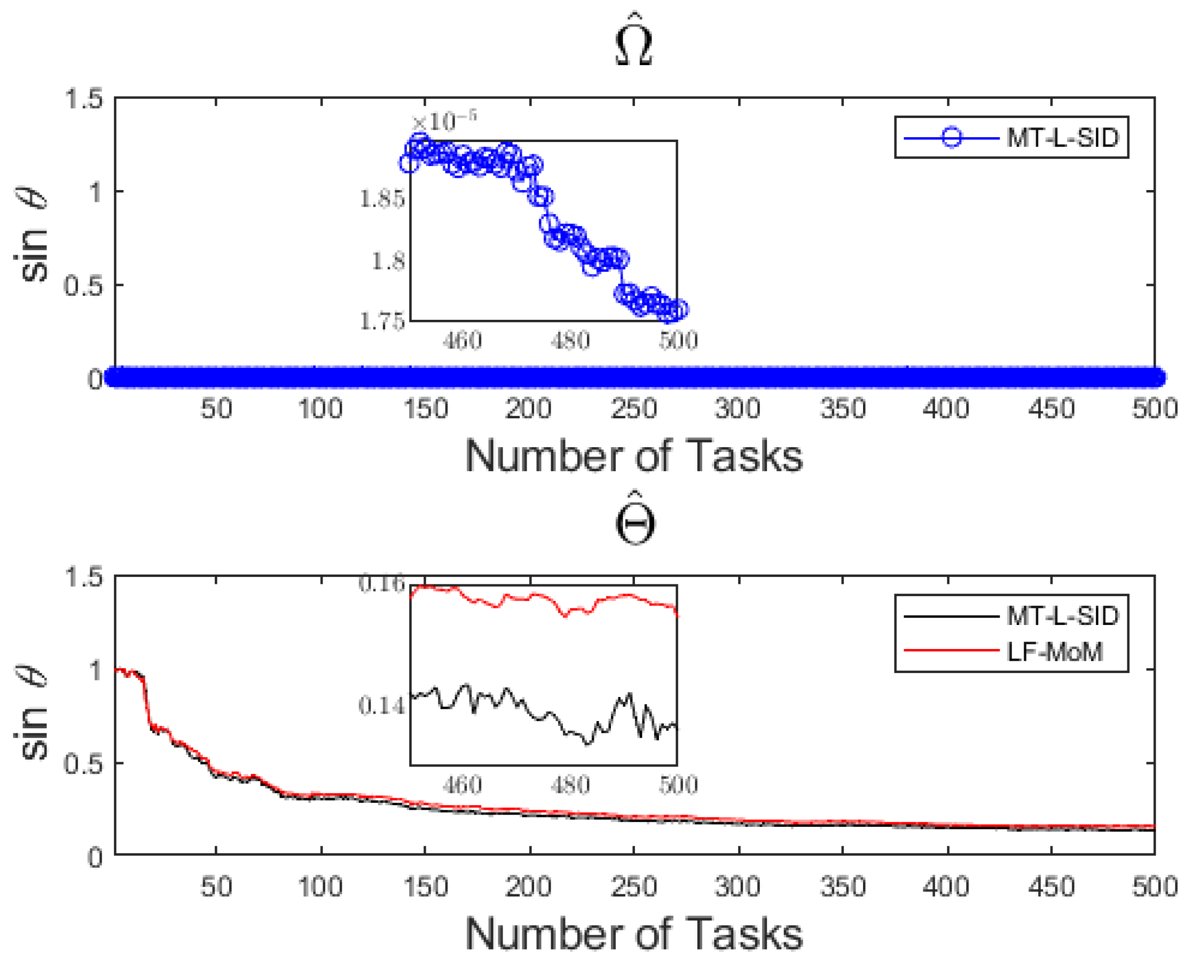
Figure 1. Sine values of principal angles between estimated and actual Ω ^ , and between estimated and actual Θ ^ , respectively, with a varying number of tasks.
Processes 11 01481 g001
Figure 2. Sine value of the principal angle between estimated and actual Ω ^ , and between the estimated and actual Θ ^ , respectively, with varying numbers of dynamic windows.
Processes 11 01481 g002
Figure 3. Comparison of poles calculated by two different models and the actual model in different training samples: (a) J G + 1 = 25 , (b) J G + 1 = 40 , and (c) J G + 1 = 100 .
Processes 11 01481 g003
Figure 4. Flowchart of IndPen fermentation process. The * in the figure represents the variable controlled by the PID controller and the highlighted variable in blue indicates that the variable can be freely selected to be recorded and used to control PAA.
Processes 11 01481 g004
Figure 5. The profile of input variables.
Processes 11 01481 g005
Figure 6. The profile of output variables.
Processes 11 01481 g006
Figure 7. Predicted outputs in operation mode 10.
Processes 11 01481 g007
Table 1. MSE calculation with different structures of common feature parameters.
N q = 1 ;
N r = 1
N q = 3 ;
N r = 3
N q = 5 ;
N r = 5
N q = 10 ;
N r = 10
N q = 15 ;
N r = 15
MT-L SID7.8861 × 10811.430532.234941.45593.605 × 106
Table 2. Input and output variables of the IndPen fermentation process.
Input VariablesOutput Variables
F a / b : Acid/base flow rate D O 2 : Dissolved oxygen conc.
F h : Heating flow rate p H : pH
F c : Cooling water flow rate T tan k : Temperature of the tank
F P A A : Phenylacetic acid flow rate C O 2 , o g : Off-gas carbon dioxide
F g : Aeration rate W : Vessel weight
F w : Water for injection flow rate O 2 , o g : Off-gas oxygen
F s : Substrate flow rate
F o i l : Oil flow rate
Table 3. Batch runs of product of each operation mode at ambient temperature condition 1.
No.Control StrategyRaman SpectroscopyInhibition
1Sequential batch controlOnly record the Raman dataDO2, T, pH, CO2, PAA, N
2Operator controller batchOnly record the Raman dataDO2, T, pH, CO2, PAA, N
3Sequential batch controlUse Raman data to control PAADO2, T, pH, CO2, PAA, N
4Operator controller batchUse Raman data to control PAADO2, T, pH, CO2, PAA, N
5Sequential batch controlUse Raman data to control PAANo inhibition
6Sequential batch controlUse Raman data to control PAADO2, T, pH
7Operator controller batchUse Raman data to control PAADO2, T, pH
8Operator controller batchUse Raman data to control PAANo inhibition
9Operator controller batchOnly record the Raman dataNo inhibition
10Sequential batch controlOnly record the Raman dataNo inhibition
11Sequential batch controlOnly record the Raman dataDO2, T, pH, CO2, PAA, N
12Operator controller batchOnly record the Raman dataDO2, T, pH, CO2, PAA, N
13Sequential batch controlUse Raman data to control PAADO2, T, pH, CO2, PAA, N
14Operator controller batchUse Raman data to control PAADO2, T, pH, CO2, PAA, N
Table 4. MSEs of SID, MT-L SID, and LF-MoM models in the IndPen fermentation process case.
SIDLF-MoMMT-L SID
Mode 1282.26382.88392.6048
Mode 229.244715.101311.7451
Mode 386.4948101.892714.5548
Mode 412.48614.53483.9649
Mode 1012.24792.45492.3101
Disclaimer/Publisher’s Note: The statements, opinions and data contained in all publications are solely those of the individual author(s) and contributor(s) and not of MDPI and/or the editor(s). MDPI and/or the editor(s) disclaim responsibility for any injury to people or property resulting from any ideas, methods, instructions or products referred to in the content.