Abstract
The Paris agreement in 2015 has required that countries commit to global carbon emission reduction by setting their national targets. In most countries, the electricity sector is identified as one of the major contributors to carbon emissions. Therefore, the governments count on decarbonizing the electricity sector to achieve their carbon reduction targets. However, this could be challenging as it is complex and involves multi-stakeholders in implementing the decarbonization plan. This work presents a mathematical optimization model to determine multi-period electricity generation planning to achieve the electricity demand and the carbon reduction target. A multi-period analysis allows long-term planning for decarbonizing the electricity sector by the gradual phasing out of coal-based power plants and the introduction of renewable-based electricity generation. To illustrate the proposed approach, the developed model is solved to strategize low-carbon energy transition planning for the Sarawak region in Malaysia. The model determines the optimal amount of new renewables required during each of the time periods, from 2020–2040, to meet the carbon reduction target. The optimal results are generated under two scenarios—no co-firing and co-firing. The generated results show that the co-firing scenario resulted in a 14.09% reduction in new renewable additions and a 5.78% reduction in the total costs. The results also determined a 66% reduction in coal consumption in 2050 when compared to the base year in 2020.
1. Introduction
The rise in atmospheric carbon dioxide (CO2) levels has led to global warming, causing climate change effects in the form of heat waves, droughts, floods, etc. The global average atmospheric CO2 in 2021 stood at a record 414.72 parts per million (ppm), which is 2.5 ppm higher than in 2020 [1]. The electricity sector remains one of the major contributors, which accounted for 25% of carbon emissions in 2021 [2]. Coal is the dominant fuel, with a 36% share in global electricity generation, followed by natural gas with 22.9% [2]. Combustion of such fossil fuels results in significant amounts of carbon emissions. On the other hand, the electricity demand is rising to meet the growing population and economy. Therefore, there is a global push for a transition towards low-carbon electricity generation.
The Paris Agreement at the Conference of Parties (COP) 21 required countries to submit carbon reduction targets called Nationally Determined Contributions (NDCs), outlaying their plans for emission reduction. To achieve thesetargets, most countries have phasing out of coal-based power plants as a key strategy. At COP 26, most countries committed to accelerate the phase-out of coal power plants while at COP 27, the countries agreed on a need to set a timeline to phase out coal power plants. In addition, a global consensus is emerging to achieve carbon neutrality between 2050 and 2070. These climate commitments require countries to phase out their coal-based electricity generation while simultaneously increasing electricity generation to meet the demand via renewable energy sources. However, one of the major challenges is to ensure energy security as they plan their decarbonization strategies. In this regard, decision support tools are necessary for policymakers to determine long-term energy sector planning. The aim of this paper is to develop a multi-period mathematical optimization model that can aid in devising strategizes to decarbonize the electricity sector.
Mathematical models and graphical methods have been developed in the past decades as effective decision support tools for long-term energy sector planning. Mathematical models can represent real-world systems and their interactions, solve large and complex problems, and effectively aid in decision making [3]. Likewise, graphical techniques, such as pinch analysis technique, can be powerful tools to draw insights for high-level decision making. The carbon emission pinch analysis (CEPA) was first presented by Tan and Foo for energy sector emission reduction planning [4]. CEPA was built upon the graphical method, pinch analysis technique, which was initially developed for heat integration in process systems [5]. It exploits the use of graphical plots to plan and allocate low-carbon energy sources to energy systems while meeting a certain amount of energy demand requirements and carbon emission reduction targets. Tan and Foo also presented a mathematical model equivalent to the graphical method in CEPA, which serves as an alternative to the graphical method [4]. Later, this was extended to a pinch targeting approach by Lee et al. while carbon capture and storage (CCS) was included in the CEPA framework by Tan et al. [6,7].
CEPA is widely used for national-level electricity sector planning for various countries. For instance, Atkins et al. extended CEPA to plan the electricity sector in New Zealand [8]. This work used CEPA to determine the amount of renewable energy sources—geothermal, wind, and hydropower—required to reduce carbon emissions and meet the projected electricity demand. Crilly and Zhelev applied CEPA to the Irish electricity sector to determine the optimal energy resource mix needed to meet the emission reduction targets [9]. Meanwhile, Jia et al. applied CEPA to identify carbon emission reduction targets for a chemical industrial park in China [10]. Priya and Bandyopadhyay presented an extended version of CEPA that included prioritized cost [11]. The extension was used to determine a trade-off between costs and emissions in identifying new power plants for the Indian electricity sector. Lim et al. then extended the use of CEPA to incorporate energy return on investment and water footprints [12]. The extended version of CEPA is used to determine the optimal energy mix required to achieve the United Arab Emirates energy demand and emission reduction plans until 2050. Besides, Baležentis et al. incorporated an ecological footprint into CEPA and used it to devise the optimal energy mix for the power sector in the three Baltic States Latvia, Estonia, and Lithuania [13]. More recently, an open-source energy systems decarbonization planning software based on the CEPA framework was developed by Nair et al. [14]. Table 1 presents a summary of countries where CEPA has been applied.

Table 1.
Variants of CEPA applied in different countries.
Apart from considering low-carbon energy resources, CEPA has also been extended to consider negative emissions technologies. For example, Tan et al. developed an extension of CEPA, which included carbon capture and storage planning [7]. Likewise, Ilyas et al. used CEPA to determine the feasibility of carbon capture retrofit in the South Korean power sector [28]. Similarly, Thengane et al. applied CEPA in planning of captured CO2 allocation to geological storage sites [29]. More recently, Nair et al. developed a CEPA approach that considered negative emission technologies for energy planning [30]. Nair et al. also extended the approach further to consider the energy penalties that come along with negative emission technologies [31].
As proven in the previous works, CEPA is user-friendly and can be easily applied to any carbon emission reduction planning scenario. Such flexibility makes CEPA easy to be integrated with other tools. For instance, Tan et al. extended the CEPA application to economic systems [32]. CEPA was combined with input–output analysis to integrate carbon reduction targets to demand side considerations. Likewise, Mu et al. applied CEPA to reduce network complexity in the P-graph of the raw material management network [33]. Moreover, Jia et al. integrated life cycle carbon accounting with CEPA to plan municipal solid waste management [15]. Li et al. also presented a framework based on CEPA to determine the minimum renewable energy target for rural areas in China [16]. The minimum renewable energy target was then used as a constraint to optimize the biomass energy supply chain in the region. Additionally, Leong et al. applied CEPA as part of a larger framework to plan carbon reduction targets and optimize the bioenergy supply chains [21]. Most recently, Mohd. Yahya et al. further extended the work by including a multi-stakeholder analysis [19]. Such analysis used the Shapley–Shubik power index to identify the level of influence each stakeholder and able to determine the optimal biomass supply chain.
Note that the previous works show that CEPA can be integrated with other methods to enhance results. However, most of the previous works assume a steady-state scenario where the energy resources and energy demands are constant. To overcome this limitation, CEPA could be enhanced further by including temporal scales in the model. With such improvement, CEPA would provide more robust and adaptive insights across a time horizon. This will allow decision makers to plan strategic carbon reduction policies for future energy demand scenarios and account for variations. A few recent CEPA extensions have considered multiple time periods. For example, Ramsook et al. presented a multi-period approach with CEPA and the developed approach was applied in a case study in Trinidad and Tobago [26]. Similarly, Kong et al. developed a multi-period CEPA to determine the optimal energy mix of fossil fuels and renewables for energy systems [34]. Although these contributions considered several time periods, the number of time periods used in those studies were still within a reasonable range for producing graphical plots. When many time periods are considered, graphical plots may be labour-intensive and impractical to produce.
Fortunately, Tan and Foo presented a mathematical model equivalent to the graphical method in CEPA which serves as an alternative to the graphical method and provides great potential for extension [4]. Based on the abovementioned literature, there is limited attention given to extending CEPA into considering biomass co-firing opportunities in coal power plants. Current CEPA variants only focus on identifying targets for low-carbon energy resources but do not go into detail on how they are utilized. Such assumption suggests that the targets are identified in CEPA for new and standalone low-carbon energy systems. However, such a system is more expensive compared to co-firing. Co-firing is important, particularly when considering a strategic phasing out of old or existing power plants in a given region. In addition, previous CEPA contributions do not account for technology selection. Such a selection is important in regional energy planning, as there are several energy generation technologies with a unique cost, efficiency, and impact on carbon reduction efforts.
Based on the detailed literature review as presented above, the following research gaps are identified:
- A multi-period CEPA will allow strategic planning for the decarbonization of the electricity sector. However, limited works have attempted a multi-period CEPA-based mathematical optimization model, and none of the works have addressed the decarbonization of Sarawak’s electricity sector;
- No previous work analyzed the effect of biomass co-firing in existing coal power plants with respect to energy demand, emission reduction targets, and costs using CEPA. Moreover, co-firing is typically factored in as a non-linear correlation in planning models, which makes them more complex to solve;
- A limited number of the previous works have accounted for technology selection within the CEPA framework;
- A limited amount of work in the literature has considered systematic strategies within the CEPA framework as an energy transition tool to phase out fossil-based power plants gradually.
This work presents an extension of CEPA’s mathematical model equivalent method. In other words, this work presents a mathematical optimization model that delivers the features found in previous CEPA contributions alongside several additional extensions. The novelty of the extended model is as follows:
- A multi-period optimization model for long-term energy planning and decarbonization strategies;
- Co-firing of biomass in coal power plants is included in the CEPA framework. A linear correlation is developed in this work to consider the co-firing performance;
- Technology selection accounting for efficiency, costs, and emissions are considered.
The following sections are organized as follows: Section 2 describes the generalized methodology for multi-period low-carbon energy transition planning and the mathematical formulations developed in this work. Next, Section 3 presents the energy transition planning for the Sarawak region based on the developed model. The results generated by the model are further discussed and analyzed in Section 4. Lastly, Section 5 draws conclusions as well as future works from this study.
2. Problem Statement
The formal problem statement is defined as below, given the following:
- A set of coal resources available for a set of coal power plants ;
- A set of biomass resources available for the coal power plants with co-firing ratio, ;
- A set of natural gas resources available for the natural gas power plants ;
- A set of diesel resources available for diesel power plants ;
- A set of hydro resources available for hydro power plants ;
- A set of time periods considered for energy planning;
- A set of regions whose electricity demand (MWh) for each of the time periods are taken for electricity sector planning;
- The emissions target, (tCO2/MWh) set for the electricity sector during each of the time periods .
The model determines the following:
- The quantity of renewables required, (MWh) to meet the electricity demand, within the set emission target, ;
- The electricity generated from the existing power plants for each of the time periods;
- The operating costs incurred at the existing power plants for each of the time periods.
The model is set with an objective to determine the quantity of renewable energy required to meet the electricity demand within the emission target at a minimum cost. The above-discussed problem requires the following input data for investigation:
- Installed capacity of the existing power plants (MWh);
- Maximum and minimum operating capacity of the power plants (MWh);
- Operations and maintenance cost of the power plants (USD/MWh);
- Efficiency of the considered power plants;
- Fuel cost of the fuel types (USD/MWh);
- Carbon emissions from each of the power plants (tCO2/MWh);
- Energy demand for the considered regions (MWh).
3. Methodology
This section presents the mathematical formulation to address the identified planning problem states in Section 2. The mathematic equations can be categorized as follows:
- Energy resource consumption;
- Operational constraint;
- Co-firing constraint;
- Energy constraint;
- Emission constraint;
- Cost estimation.
3.1. Energy Resource Consumption
The energy resource consumption at the power plants can be determined as shown in Equation (1). The consumption of the coal resource c at the coal power plant cp during the time period t, (MWh) can be determined as shown in Equation (1).
where is the electricity generated from coal power plant cp using the coal resource c to meet the energy demand at region l for the time period t. refers to the efficiency of the coal power plant cp that operates using the coal resource c for the time period t. Similarly, the consumption of biomass, natural gas, diesel, and hydro resources can be determined using Equations (2)–(5).
3.2. Operational Constraint
The maximum electricity generation capacity of the power plants is given by their installed capacity. For example, the installed capacity of the coal power plant cp for the time period t is given by . However, the power plant may not necessarily operate at its installed capacity for all the time periods. In this work, the maximum and minimum operating capacity of the power plants for each of the time periods is assigned by the maximum capacity factor, u, and the minimum capacity factor, v. The minimum (economically feasible) capacity factor, v, constrains the model from shutting down fossil-based power plants instantly. Likewise, the maximum capacity factor, u, can be gradually decreased across the time period t to model the systematic phasing out of fossil-based power plants. Thus, the capacity factor values, u and v, can be determined by the decision maker to devise strategic plans to phase out the fossil-based power plants based on the economic performance of individual plants, environmental considerations, etc. The maximum and minimum operating capacity constraints are set as shown in Equations (6)–(9).
3.3. Co-Firing Constraint
Co-firing allows using a secondary fuel to be used along with the primary fuel in power plants. Typically, the secondary fuel may be cheaper or more environmentally friendly. For example, a co-firing biomass pellet which has reasonably high energy content can be cofired with coal in power plants. However, to ensure the performance of the power plant, co-firing requires to be guided by a parameter called co-firing ratio, . Co-firing biomass beyond the prescribed limit may result in reduced performance at the power plant. Therefore, co-firing constraint is modelled as shown in Equation (10).
3.4. Energy Constraint
The electricity demand of region l for each of the time periods t is to be met by the electricity supply from all of the power plants as shown in Equation (11).
where (MWh) is the renewables required to meet the electricity demand within the emission target. The inclusion of multiple time periods allows accounting for the increasing electricity demands and stringent emission targets in formulating a long-term decarbonization strategy.
3.5. Emission Constraint
The emission constraint shown in Equation (12) is the key constraint used in the CEPA methodology. It essentially represents the equality between the emissions generated by the power plants and the emission target. is the carbon emission from the coal power plant cp operated using the coal resource c during the time period t. The carbon emissions from the rest of the power plants are denoted like the one shown for coal. The carbon emission target set for electricity generation to be supplied for region l during the time period t is given by .
3.6. Cost Estimation
The operating cost of the existing power plants accounts for the operations and maintenance cost (O&M cost) and fuel cost. The operating cost of the coal power plant cp during the time period t, (USD) can be determined as shown in Equation (13).
Similarly, the operating costs at natural gas power plants, diesel power plants, and hydro power plants can be determined as shown in Equations (14)–(16).
The proposed optimization model determines the renewable energy generation (MWh) required to meet the electricity demand within the emission target. The cost of the renewables is estimated by considering the levelized cost of energy (LCOE) for renewable-based electricity generation. LCOE refers to the price at which the electricity needs to be sold to recover the total investment of setting up the power plant. Though LCOE does not reflect the capital and operating costs of generating electricity from renewables, it captures the cost trends in adding renewables to the energy mix. The cost of renewables is estimated as shown in Equation (17). The total cost involved in electricity generation for the time period t can be determined as shown in Equation (18).
Finally, the optimization objective of this model is set to minimize the total cost as shown in Equation (19).
4. Low-Carbon Energy Transition Planning for Sarawak
This section presents the low-carbon energy transition planning for the Sarawak region based on the mathematical optimization model presented in Section 3. Sarawak is the largest state in Malaysia with an area of 124,450 sq. km and a population of 2,907,000 in 2020 [35]. It has an abundance of indigenous natural resources like hydro and biomass. Sarawak has the potential to use biomass for co-firing in coal power plants and hence co-firing is an important option to account for during the coal phase-out strategy. Recently, the Post COVID-19 Development Strategy 2030 document by the Sarawak government also mandated to increase the renewable energy capacity [36]. Therefore, this work aims to present the application of the model developed in Section 3 in planning the decarbonization of Sarawak’s electricity sector with an emphasis on biomass co-firing.
Based on the data collected through stakeholder engagement and the literature review, the list of power plants operated and planned in Sarawak is presented in Table 2. This case study aims to determine the optimal renewable energy generation required during each of the time periods to meet the electricity demand within the emission limit. The equations presented in Section 3 are modeled in AIMMS which of the mathematical class—mixed integer linear programming (MILP) and solved in a 64-bit HP Pavilion x360 computer with Intel® CoreTM i5 8250 processor and 8 GB RAM.
Table 2.
List of power plants in Sarawak, Malaysia [37].
A long-term planning horizon is considered in this case study for every five years from 2016 to 2040. A five-year time interval is the usual practice of the Malaysian government to set economic targets and devise policies accordingly. Therefore, the values used and reported in this work are the result at the end of each of the five years (i.e., 2020, 2025, 2030, 2035, and 2040). All the assumptions made in this case study are listed below:
- All the power plants are assumed to be operating for 8000 h annually;
- The efficiency of the power plants based on different energy sources is assumed to be constant throughout the years unless new technologies are introduced. In this work, the efficiency for biomass co-firing in coal power plants is assumed to be 30%;
- The operating and maintenance cost of the power plants is assumed to remain constant as business as usual throughout the years;
- It is assumed that biomass and hydro resources have negligible carbon emissions due to the nature of such renewable energy sources. Biomass is taken from agricultural waste and hydro power does not consume fossil fuels during the operation;
- The carbon emission factor is assumed to remain constant for each type of energy source throughout the years;
- Water resource for hydro power plants is assumed to have no feedstock cost.
The electricity generation capacities of the power plants for each of the time periods are shown in Table 3. It should be noted that the capacity of the NG2 plant increases from 2025 onwards due to the expected commencement of two new additional combined-cycle blocks. Similarly, the H4 plant is currently under construction and is expected to commence production from 2026 onwards.
Table 3.
Maximum capacity of each power plant (MWh).
Table 4 shows the operating range of each power plants over the time periods. The operating range represents the maximum and minimum percentage of the installed capacity within which the power plants can operate. As mentioned in Section 2, the operating range is set based on the strategy to phase out fossil fuel plants systematically. These values are gradually decreased across the time planning horizon to depict the strategic phasing out. Such a strategy will prevent immediate shutdowns of plants at the start of the time horizon to meet the carbon reduction target, thereby offering a practical and realistic decarbonization strategy.
Table 4.
Operating range of each of the power plants.
Based on the conversion technology, the efficiencies of the power plant considered in this case study are shown in Table 5. As presented previously in the assumption, the efficiency of co-firing biomass in coal power plants is taken as 30% and constant throughout the years unless new technologies are introduced. The efficiency of NG2 is taken at 28.1% from 2025 onwards due to the addition of two new combined cycle blocks. Furthermore, the operation and maintenance (O&M) cost at the power plant is also provided in Table 5. Table 6 shows the fuel cost factor incurred to keep the power plants running. Note that the fuel cost of coal, natural gas and biomass are projected based on Sönnichsen [38]. Meanwhile, the cost of diesel in 2020 is obtained from the US Energy Information Administration and the values for subsequent years are projected accordingly [39].
Table 5.
Efficiency and O&M costs (USD/MWh) of the power plants.
Table 6.
Fuel costs of each energy resource (USD/MWh).
Table 7 summarized all the emission factor of each power plant. Note that the emission factor mainly depends on the type of fuel source. Moreover, the unique efficiencies of power plants with the same fuel source also result in different emission factors.
Table 7.
Emission factor of each power plant (tCO2/MWh).
Based on the engagement with industry partners and local utility’s projection, Table 8 shows the projected electricity demand for the Sarawak region in Malaysia. The electricity demands for the upcoming time periods were estimated using the projected values with the overall electricity demand trend. The data obtained from Sarawak Energy’s Annual & Sustainability Report 2019 are used in the first time period (i.e., 2020) as base values [40]. In addition, the carbon reduction targets for the region set to evaluate the performance of the developed model. The carbon reduction targets are fixed in decreasing order over the years to depict a carbon reduction strategy that spans the time horizon. However, it can be seen in Table 8 that the carbon target factor increases temporarily in 2025 before reducing again over the rest of the years. This accounts for the additional carbon emission from the two new combined-cycle blocks in the NG2 plant. These plants were projects scheduled for 2020 and expected to run by 2025.
Table 8.
Projected electricity demand and carbon reduction targets.
5. Results
In solving the developed model with the case study information in Section 4, the optimized results are presented in Table 9. The renewable energy generation required during each of the time periods for both scenarios are presented. As shown, the total renewable generation required for Scenario 1 is 18.38 million MWh while for Scenario 2 is 15.79 million MWh. Co-firing in Scenario 2 allowed a 14.09% reduction in new renewable energy generation. Table 10 compares the total costs between non-co-firing and co-firing scenarios. The total cost of Scenario 1 is USD 5.02 trillion and that of Scenario 2 is USD 4.73 trillion. Co-firing has resulted in cost savings of USD 293.09 million, which is reduction of 5.78% from Scenario 1.
Table 9.
Renewable-based energy generation required (MWh).
Table 10.
Total cost comparison (million USD).
The varied requirement for renewable energy generation between the two scenarios implies variation in energy generation from the existing power plants. Table 11 and Table 12 show the energy generation from each of the power plants for Scenario 1 and Scenario 2, respectively. As expected, the general trend that can be observed is the reduction in energy generation from fossil-based power plants over time periods. An increased energy generation from NG2 can be noticed in 2025 in both scenarios because of new capacity additions. Likewise, the increased generation seen at D4 (2025) and D8 (2025, 2030) in both scenarios is due to capacity additions. However, in all the above three cases, the increased energy generation is still below the installed capacity. In Scenario 2, an increase in generation from the preceding time period can be observed at C2 in 2035, C4 in 2035, D1 in 2030, and D8 in 2040.
Table 11.
Energy generation from existing power plants—Scenario 1 (MWh).
Table 12.
Energy generation from existing power plants—Scenario 2 (MWh).
The quantity of energy resources required for electricity generation from the power plants is presented in Table 13 for Scenario 1 and Table 14 for Scenario 2. The fossil-based energy resources are provided in MWh while the hydro resource is given in cubic meters. It is noted in Table 14 that the model decides to co-fire from 2020 onwards. However, during 2030, power plants C1, C3, and C4 operated only with coal due to the commissioning of hydro power plant, H4. Since Scenario 1 is non-co-firing, no biomass resource is consumed at coal power plants.
Table 13.
Energy resource requirement at each of the power plants—Scenario 1 (MWh).
Table 14.
Energy resource requirement at each of the power plant—Scenario 2 (MWh).
6. Discussion
This section analyzes and compares the results generated from the two energy planning scenarios (i.e., S1—non-co-firing, S2—co-firing). Figure 1 shows the electricity generation from the existing power plants and the electricity required from renewables for both scenarios for each of the time periods. The energy demand can be met within the emission limits for the 2020 period with no new renewables required. However, the existing power plants are not sufficient to meet the energy demand within the emission limits from 2025 onwards. As expected, the scenario comparison for each time period shows that Scenario 2 requires lower renewable energy to meet the emission targets of Scenario 1. Scenario 2 requires 22%, 20%, and 6.5% lesser renewables during 2025, 2035, and 2040 when compared to Scenario 1. Scenario 2 does not require renewables in 2030 due to the commencement of new hydro power plants, while Scenario 1 requires 89,388.73 MWh during the same period.
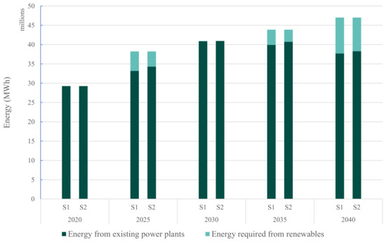
Figure 1.
Energy generation from existing power plants and new renewables.
Figure 2 shows the electricity generation from existing power plants by fuel source. Hydro power plants are the dominant source of electricity generation in Sarawak due to abundant hydro resources and suitable topography. The contribution from hydro power plants has increased from 2030 onwards due to the commencement of H4. Similarly, the contribution of natural gas power plants has increased from 2025 onwards due to capacity addition at NG2. Figure 3 shows the distribution of electricity generation by fuel source across the time periods. A gradual decline in the generation of coal power plants from 14.25% in 2020 to 1.45% (Scenario 1) in 2040. Co-firing (Scenario 2) has allowed a marginally higher share of coal power plants, with a contribution of 4.25% in 2040. A declining share of natural gas power plants in the energy mix can be also observed. In the case of Scenario 2, the percentage share has dropped to 9.24% in 2040 from as high as 23% in 2025. The share of hydro power plants remains stable at around 70% due to full capacity utilization on account of zero carbon emissions. The contribution of the diesel power plants is very negligible at 0.20%. The share of renewables has increased from 0% in 2020 to 19.8% for Scenario 1 and 18.5% in Scenario 2 in 2040.
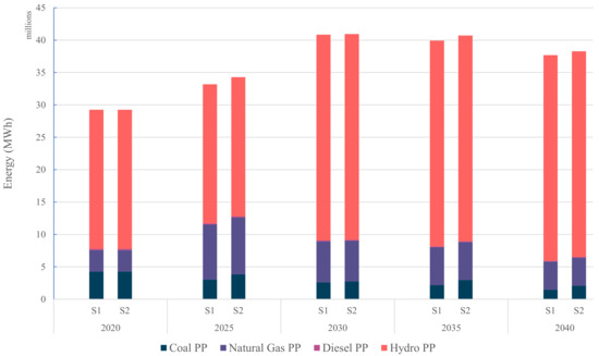
Figure 2.
Energy generation by fuel source.
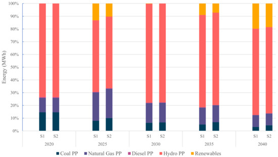
Figure 3.
Distribution of energy generation by fuel source.
Figure 4 presents the energy generation from the individual coal power plants for the time periods and compares the two scenarios. As shown, there exist four coal power plants with a total installed capacity of 4.27 million MWh. The total energy generation from all the coal plants in Scenario 1 is 4.27, 3.03, 2.60, 2.18, and 1.45 million MWh, while that of Scenario 2 is 4.27, 3.84, 2.72. 2.99, and 2.06 million MWh during 2020, 2025, 2030, 2035, and 2040, respectively.
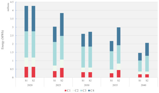
Figure 4.
Energy generation from coal power plants.
The operating range of the coal power plants across time periods is shown in Figure 5. The blue line depicts Scenario 1 while the yellow line represents Scenario 2 in Figure 5. Scenario 2 has resulted in a higher operating capacity of coal power plants than Scenario 1 across the time periods due to co-firing. Interestingly, Scenario 2 records a higher operating capacity in 2035 at plants C1, C2, and C3 than in 2030 due to the commencement of hydro power plant, H4. The generation from H4 enables it to meet the emission limits with the higher operating capacity of coal plants. By 2040, C1 and C2 operate at their minimum operating range of 30% for both scenarios. C3 and C4 operate at 42 and 30% capacity in Scenario 1 while they operate at higher capacities of 60 and 51% in Scenario 2 during 2040. The results show the successful implementation of the strategy to gradually phase out the coal usage in the existing power plants. In addition to new renewable capacity addition, co-firing has allowed the operation of existing coal power plants in achieving the electricity demand within the emission targets.
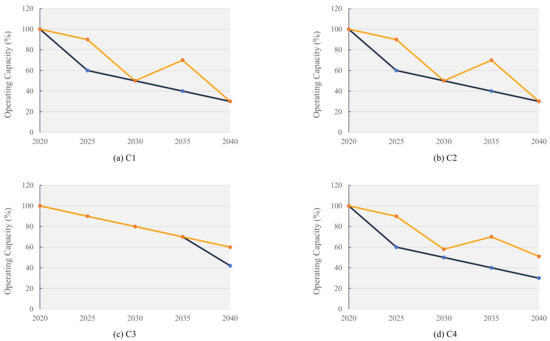
Figure 5.
Operating range of coal power plants.
The electricity generated from the natural gas power plants is shown in Figure 6. The total installed capacity of natural gas plants was 3.13 million MWh in 2020 and increased to 9.92 million MWh from 2025 onwards. The total energy generation from all natural gas plants in Scenario 1 is 3.31, 8.51, 6.34, 5.84, and 4.34 million MWh, while in Scenario 2 it is 3.31, 8.80, 6.31, 5.83, and 4.34 million MWh during 2020, 2025, 2030, 2035, and 2040, respectively. Unlike the coal plants, the difference in generation from natural gas plants between the two scenarios is small. Therefore, the plants also operate at similar capacities for both scenarios, except in 2025 when capacity utilization is marginally higher in Scenario 2 (90%) when compared to Scenario 1 (86%) as shown in Figure 7. This could be attributed to the co-firing in Scenario 2, allowing natural gas plants to operate at a marginally higher capacity within the emission limits. The operating capacity of the plants NG1, NG2, and NG3 in 2040 is 60%, 40%, and 30% for both scenarios, indicating a steady decline of generation from natural gas plants.
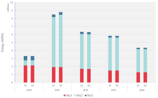
Figure 6.
Energy generation from natural gas power plants.
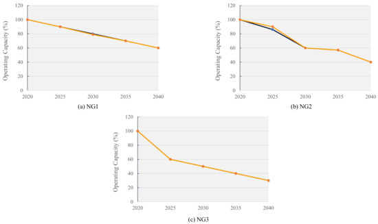
Figure 7.
Operating capacity of natural gas power plants.
As previously discussed, the total electricity generation from diesel power plants is negligible and therefore, it is not considered for detailed analysis. The electricity generation from the hydro power plants H1, H2, H3, and H4 is shown in Figure 8. The total installed capacity of hydro plants was 21.50 million MWh in 2020 and 2025 and later increased to 31.78 million MWh from 2030 onwards. All the hydro plants operate at full capacity across all time periods due to zero operational emissions during electricity generation.
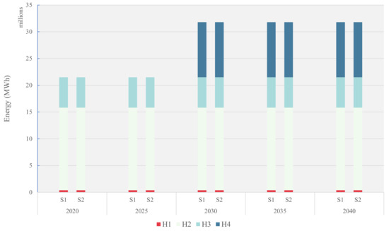
Figure 8.
Energy generation from hydro power plants.
The energy resource required for electricity generation is previously presented in Table 13 and Table 14 in Section 4. However, the data in these tables are presented in MWh. The equivalent physical quantity of the energy source is determined with the following energy content values: coal—20 MJ/kg, biomass—15 MJ/kg, natural gas—40 MJ/m3, and diesel—5564.55 MJ/barrel. The quantity of energy sources consumed during each of the time periods is shown in Table 9. The blue line represents the Scenario 1 values while the green line shows the Scenario 2 values. Scenario 2 consumes a lower quantity of coal in 2020 and 2025, whereas both Scenario 1 and Scenario 2 consume the same quantity from 2030 onwards as shown in Figure 9a. However, in addition to coal, Scenario 2 also consumes biomass which results in higher capacity utilization of coal power plants. The total coal consumption in Scenario 1 is 7.48 million tons while in Scenario 2 is 6.67 million tons, a reduction of 0.81 million tons of coal. Co-firing has reduced around 10% of coal consumption at coal power plants. Scenario 2, with co-fired biomass, requires a total quantity of 3.06 million tons. The natural gas consumption in 2020 was 974.25 million m3. This peaked at 2.57 billion m3 in 2025 and then gradually reduced to 1.28 billion m3 by 2040 as can be seen in Figure 9b. The diesel consumption at diesel power plants has been reduced from 334,382 barrels in 2020 to 200,765 barrels in Scenario 1, and 194,238 barrels in Scenario 2 by 2040 as shown in Figure 9c.
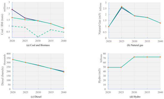
Figure 9.
Energy resource consumption.
The total cost for each time period is discussed already in Table 2. Furthermore, the cost breakdown by fuel source is shown in Figure 10. The cost values discussed below are in the following order of time periods—2020, 2025, 2030, 2035, and 2040. The operating cost of coal power plants for Scenario 1 is USD 302.73 million, USD 77.44 million, USD 65.94 million, USD 55.33 million, and USD 38.20 million, and for Scenario 2 it is USD 287.71 million, USD 123.12 million, USD 70.09 million, USD 86.72 million, and USD 58.81 million. The steep reduction in costs at coal power plants in 2025 is due to the high fuel cost of coal during the base year, 2020. The cost incurred at natural gas plants in Scenario 1 is USD 92.41 million, USD 360.62 million, USD 281.71 million, USD 263.84 million, and USD 194.61 million, while for Scenario 2 it is USD 92.41 million, USD 373.80 million, USD 280.51 million, USD 263.32 million, and USD 194.61 million. The increase in the cost that incurred at natural gas power plants from 2025 onwards is due to capacity addition at NG2. The diesel power plant costs were a meager USD 2.12 million in 2020 and further decreased to less than 1 million in both scenarios by 2040. The cost at hydro power plants for both scenarios for each of the time periods is USD 81.32 million, USD 81.32 million, USD 119.67 million, USD 119.67 million, and USD 119.67. million. The hydro power plants incur the least cost though it contributes the highest share in energy generation.
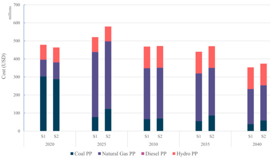
Figure 10.
Cost breakdown by fuel source.
As discussed in Section 3.6, the cost of renewables is estimated by considering the LCOE. The objective of this work is set to minimize the total cost. Hence, in this case, the determination of renewables required is dependent on the value of LCOE considered. A change in the LCOE value may have an impact on the electricity generation from each of the individual power plants and the renewables required. This work has taken the LCOE value of renewable generation to be USD 150/MWh. A sensitivity analysis is performed between LCOE values (USD 25—200/MWh) and the renewables required, and the results are presented for each of the time periods in Figure 11. The dotted line refers to the electricity generated from the existing power plants while the normal line refers to electricity generated from renewables.
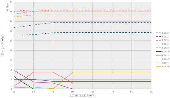
Figure 11.
Sensitivity analysis—LCOE vs. Energy generation.
It can be observed from Figure 11 that the amount of new renewables required during each time period varies based on the LCOE. Moreover, as expected, the model determines higher capacity utilization of the existing power plants when the LCOE of renewables increases. When the LCOE reaches USD 25/MWh, new renewables are added for each time period. However, when the LCOE reaches USD 100/MWh and above, new renewables are added only during the periods 2025, 2035, and 2040.
7. Conclusions
This work presented a mathematical model to determine an optimal low-carbon energy transition planning for the Sarawak region in Malaysia. The developed model was based on the carbon emission pinch analysis (CEPA) method. The model allows decision makers to devise electricity generation plans from different sources based on the demand and carbon reduction targets. It determines the amount of low-carbon energy generation required and the co-firing opportunities to meet the carbon reduction targets. The optimal energy planning strategies from 2020 to 2040 were determined under two scenarios—no co-firing and co-firing. Key insights such as the amount of new renewables required for each of the time periods, electricity generation from existing power plants for each of the time periods, and their corresponding costs are obtained. The co-firing scenario resulted in 14.09% lesser new renewables and a 5.78% lower cost compared to the non-co-firing scenario. Future works can include other emerging technologies that could be vital for a transition towards net zero emission. For instance, besides co-firing biomass, standalone bioenergy with carbon capture and storage (BECCS) can also be considered in future works. Furthermore, co-firing of natural gas power plants with biomethane and green hydrogen is also worthy for subsequent analysis. Future works can also incorporate energy storage in regional energy planning works with additional low-carbon resources as the basis. Aside from this, emerging technologies such as negative emission technologies can be considered in the model to target further carbon emission reductions.
Author Contributions
Conceptualization: V.A., Y.K.W. and D.K.S.N.; methodology: J.P.R., N.N.S. and V.A.; software: J.P.R. and N.N.S.; validation: V.A., Y.K.W. and D.K.S.N.; formal analysis: J.P.R. and V.A.; investigation: J.P.R.; resources: V.A. and N.N.S.; data curation: N.N.S. and J.P.R.; writing—original draft preparation: J.P.R. and N.N.S.; writing—review and editing: V.A., Y.K.W. and D.K.S.N.; visualization: J.P.R. and V.A.; supervision: V.A. and Y.K.W. All authors have read and agreed to the published version of the manuscript.
Funding
This research received no external funding.
Data Availability Statement
Data are available in a publicly accessible repository that does not issue DOIs. These data can be found at https://meih.st.gov.my/documents/10620/19759/National+Energy+-Balance+2019 (accessed on 4 May 2023).
Conflicts of Interest
The authors declare no conflict of interest.
Nomenclature
| Indices | |
| Fuel type | |
| Index for coal resource | |
| Index for biomass resource | |
| Index for natural gas resource | |
| Index for diesel resource | |
| Index for hydro resource | |
| Power plants | |
| Index for coal power plants | |
| Index for natural gas power plants | |
| Index for diesel power plants | |
| Index for hydro power plants | |
| Index for time period | |
| Index for region or location | |
| Parameters | |
| Efficiency of coal power plant cp operated with coal resource c for the time period t (%) | |
| Efficiency of coal power plant cp operated with biomass resource b for the time period t (%) | |
| Efficiency of natural gas power plant ngp with natural gas resource ng for the time period t (%) | |
| Efficiency of diesel power plant dp with diesel resource d for the time period t (%) | |
| Efficiency of hydro power plants hp with hydro resource h for the time period t (%) | |
| Installed capacity of coal power plants (MWh) | |
| Installed capacity of natural gas power plants (MWh) | |
| Installed capacity of diesel power plants (MWh) | |
| Installed capacity of hydro power plants (MWh) | |
| Maximum capacity factor of coal power plants (%) | |
| Maximum capacity factor of natural gas power plants (%) | |
| Maximum capacity factor of diesel power plants (%) | |
| Maximum capacity factor of hydro power plants (%) | |
| Minimum capacity factor of coal power plants (%) | |
| Minimum capacity factor of natural gas power plants (%) | |
| Minimum capacity factor of diesel power plants (%) | |
| Minimum capacity factor of hydro power plants (%) | |
| Co-firing ratio at coal power plants | |
| Energy demand at region l for time-period t (MWh) | |
| Carbon emission target for region l during time period t (tCO2/MWh) | |
| Carbon emissions from coal power plants (tCO2/MWh) | |
| Carbon emissions from natural gas power plants (tCO2/MWh) | |
| Carbon emissions from diesel power plants (tCO2/MWh) | |
| Carbon emissions from hydro power plants (tCO2/MWh) | |
| O&M cost at coal power plants (USD/MWh) | |
| O&M cost at natural gas power plants (USD/MWh) | |
| O&M cost at diesel power plants (USD/MWh) | |
| O&M cost at hydro power plants (USD/MWh) | |
| Fuel cost of coal at coal power plants (USD/MWh) | |
| Fuel cost of biomass at coal power plants (USD/MWh) | |
| Fuel cost at natural gas power plants (USD/MWh) | |
| Fuel cost at diesel power plants (USD/MWh) | |
| Fuel cost at hydro power plants (USD/MWh) | |
| Levelized cost of energy for renewables (USD/MWh) | |
| Variables | |
| Coal consumption at coal power plants (MWh) | |
| Biomass consumption at coal power plants (MWh) | |
| Natural gas consumption at natural gas power plants (MWh) | |
| Diesel consumption at diesel power plants (MWh) | |
| Water consumption at hydro power plants (MWh) | |
| Electricity generated from coal power plant using coal resource (MWh) | |
| Electricity generated from coal power plant using biomass resource (MWh) | |
| Electricity generated from natural gas power plant (MWh) | |
| Electricity generated from diesel power plant (MWh) | |
| Electricity generated from hydro power plant (MWh) | |
| Renewables required (MWh) | |
| Operating cost at coal power plants (MWh) | |
| Operating cost at natural gas power plants (MWh) | |
| Operating cost at diesel power plants (MWh) | |
| Operating cost at hydro power plants (MWh) | |
| Estimated cost of renewables for the time period t (MWh) | |
| Total cost of electricity generation for the time period t (MWh) |
References
- Lindsey, R. Atmospheric Carbon Dioxide. 2020. Available online: https://www.climate.gov/news-features/understanding-climate/climate-change-atmospheric-carbon-dioxide (accessed on 20 April 2023).
- IEA. Global Energy Review: CO2 Emissions in 2021. 2021. Available online: https://www.iea.org/reports/global-energy-review-co2-emissions-in-2021-2 (accessed on 3 March 2023).
- Andiappan, V. State-of-the-art review of mathematical optimisation approaches for synthesis of energy systems. Process Integr. Optim. Sustain. 2017, 1, 165–188. [Google Scholar] [CrossRef]
- Tan, R.R.; Foo, D.C.Y. Pinch analysis approach to carbon-constrained energy sector planning. Energy 2007, 32, 1422–1429. [Google Scholar] [CrossRef]
- Linnhoff, B.; Flower, J.R. Synthesis of heat exchanger networks: I. Systematic generation of energy optimal networks. AIChE J. 1978, 24, 633–642. [Google Scholar]
- Lee, C.S.; Ng, D.K.S.; Foo, D.C.Y.; Tan, R.R. Extended Pinch Targeting Techniques for Carbon-Constrained Energy Sector Planning. Appl. Energy 2009, 86, 60–67. [Google Scholar] [CrossRef]
- Tan, R.R.; Ng, D.K.S.; Foo, D.C.Y. Pinch Analysis Approach to Carbon-Constrained Planning for Sustainable Power Generation. J. Clean. Prod. 2009, 17, 940–944. [Google Scholar] [CrossRef]
- Atkins, M.J.; Morrison, A.S.; Walmsley, M.R.W. Carbon Emissions Pinch Analysis (CEPA) for emissions reduction in the New Zealand electricity sector. Appl. Energy 2010, 87, 982–987. [Google Scholar] [CrossRef]
- Crilly, D.; Zhelev, T. Further emissions and energy targeting: An application of CO2 emissions pinch analysis to the Irish electricity generation sector. Clean Technol. Environ. Policy 2010, 12, 177–189. [Google Scholar] [CrossRef]
- Jia, X.; Liu, C.-H.; Qian, Y. Carbon Emission Reduction using Pinch Analysis. In Proceedings of the 4th International Conference on Bioinformatics and Biomedical Engineering, Chengdu, China, 18–20 June 2010. [Google Scholar]
- Priya, G.S.K.; Bandyopadhyay, S. Emission constrained power system planning: A pinch analysis based study of Indian electricity sector. Clean Technol. Environ. Policy 2013, 15, 771–782. [Google Scholar] [CrossRef]
- Lim, X.Y.; Foo, D.C.Y.; Tan, R.R. Pinch analysis for the planning of power generation sector in the United Arab Emirates: A climate-energy-water nexus study. J. Clean. Prod. 2018, 180, 11–19. [Google Scholar] [CrossRef]
- Baležentis, T.; Štreimikienė, D.; Melnikienė, R.; Zeng, S. Resources, Conservation & Recycling Prospects of green growth in the electricity sector in Baltic States: Pinch analysis based on ecological footprint. Resour. Conserv. Recycl. 2019, 142, 37–48. [Google Scholar]
- Nair, P.N.S.B.; Tan, R.R.; Foo, D.C.; Gamaralalage, D.; Short, M. DECO2—An Open-Source Energy System Decarbonisation Planning Software including Negative Emissions Technologies. Energies 2023, 16, 1708. [Google Scholar] [CrossRef]
- Jia, X.; Wang, S.; Li, Z.; Wang, F.; Tan, R.R.; Qian, Y. Pinch analysis of GHG mitigation strategies for municipal solid waste management: A case study on Qingdao City. J. Clean. Prod. 2018, 174, 933–944. [Google Scholar] [CrossRef]
- Li, Z.; Jia, X.; Foo, D.C.Y.; Tan, R.R. Minimizing carbon footprint using pinch analysis: The case of regional renewable electricity planning in China. Appl. Energy 2016, 184, 1051–1062. [Google Scholar] [CrossRef]
- Walmsley, M.R.W.; Walmsley, T.G.; Atkins, M.J.; Kamp, P.J.J.; Neale, J.R. Minimising carbon emissions and energy expended for electricity generation in New Zealand through to 2050. Appl. Energy 2014, 135, 656–665. [Google Scholar] [CrossRef]
- Sinha, R.K.; Chaturvedi, N.D. A graphical dual objective approach for minimizing energy consumption and carbon emission in production planning. J. Clean. Prod. 2018, 171, 312–321. [Google Scholar] [CrossRef]
- Mohd Yahya, N.S.; Ng, L.Y.; Andiappan, V. Optimisation and planning of biomass supply chain for new and existing power plants based on carbon reduction targets. Energy 2021, 237, 121488. [Google Scholar] [CrossRef]
- Ramli, A.F.; Muis, Z.A.; Ho, W.S.; Idris, A.M.; Mohtar, A. Carbon Emission Pinch Analysis: An application to the transportation sector in Iskandar Malaysia for 2025. Clean Technol. Environ. Policy 2019, 21, 1899–1911. [Google Scholar] [CrossRef]
- Leong, H.; Leong, H.; Foo, D.C.Y.; Yin Ng, L.; Andiappan, V. Hybrid approach for carbon-constrained planning of bioenergy supply chain network. Sustain. Prod. Consum. 2019, 18, 250–267. [Google Scholar] [CrossRef]
- Salman, B.; Nomanbhay, S.; Foo, D.C.Y. Carbon emissions pinch analysis (CEPA) for energy sector planning in Nigeria. Clean Technol. Environ. Policy 2018, 21, 93–108. [Google Scholar] [CrossRef]
- De Lira Quaresma, A.C.; Francisco, F.S.; Pessoa, F.L.P.; Queiroz, E.M. Carbon emission reduction in the Brazilian electricity sector using Carbon Sources Diagram. Energy 2018, 159, 134–150. [Google Scholar] [CrossRef]
- Walmsley, M.R.W.; Walmsley, T.G.; Atkins, M.J. Achieving 33% renewable electricity generation by 2020 in California. Energy 2015, 92, 260–269. [Google Scholar] [CrossRef]
- Cossutta, M.; Foo, D.C.Y.; Tan, R.R. Carbon emission spinch analysis (CEPA) for planning the decarbonization of the UK power sector. Sustain. Prod. Consum. 2021, 25, 259–270. [Google Scholar] [CrossRef]
- Ramsook, D.; Boodlal, D.; Maharaj, R. Multi-period Carbon Emission Pinch Analysis (CEPA) for reducing emissions in the Trinidad and Tobago power generation sector. Carbon Manag. 2022, 13, 164–177. [Google Scholar] [CrossRef]
- Lopez, N.S.A.; Foo, D.C.Y.; Tan, R.R. Optimizing regional electricity trading with Carbon Emissions Pinch Analysis. Energy 2021, 237, 121544. [Google Scholar] [CrossRef]
- Ilyas, M.; Lim, Y.; Han, C. Pinch based approach to estimate CO2 capture and storage retrofit and compensatory renewable power for South Korean electricity sector. Korean J. Chem. Eng. 2012, 29, 1163–1170. [Google Scholar] [CrossRef]
- Thengane, S.K.; Tan, R.R.; Foo, D.C.Y.; Bandyopadhyay, S. A Pinch-Based Approach for Targeting Carbon Capture, Utilization, and Storage Systems. Ind. Eng. Chem. Res. 2019, 58, 3188–3198. [Google Scholar] [CrossRef]
- Nair, P.N.S.B.; Tan, R.R.; Foo, D.C.Y. Extended Graphical Approach for the Deployment of Negative Emission Technologies. Ind. Eng. Chem. Res. 2020, 59, 18977–18990. [Google Scholar] [CrossRef]
- Nair, P.N.S.B.; Tan, R.R.; Foo, D.C.Y. Extended graphical approach for the implementation of energy-consuming negative emission technologies. Renew. Sustain. Energy Rev. 2022, 158, 112082. [Google Scholar] [CrossRef]
- Tan, R.R.; Aviso, K.B.; Foo, D.C.Y. Carbon emissions pinch analysis of economic systems. J. Clean. Prod. 2018, 182, 863–871. [Google Scholar] [CrossRef]
- Mu, P.; Yang, Y.; Han, Y.M.; Gu, X.; Zhu, Q.X. Raw material management networks based on an improved P-graph integrated carbon emission pinch analysis (CEPA-P-graph) method. Can. J. Chem. Eng. 2020, 98, 676–689. [Google Scholar] [CrossRef]
- Kong, K.G.H.; How, B.S.; Lim, J.Y.; Leong, W.D.; Teng, S.Y.; Ng, W.P.Q.; Moser, I.; Sunarso, J. Shaving electric bills with renewables? A multi-period pinch-based methodology for energy planning. Energy 2022, 239, 122320. [Google Scholar] [CrossRef]
- The Official Portal of Sarawak Government. Available online: https://sarawak.gov.my/web/home/article_view/240/175/?id=158#175 (accessed on 20 April 2023).
- Post COVID-19 Development Strategy 2030, 2022. Economic Planning Unit, Sarawak Government. Available online: https://sarawak.gov.my/media/attachments/PCDS_-Compressed_22_July_2021.pdf (accessed on 20 April 2023).
- National Energy Balance (NEB), 2019. Energy commission, Government of Malaysia. Available online: https://meih.st.gov.my/documents/10620/19759/National+Energy+-Balance+2019 (accessed on 20 April 2023).
- Sönnichsen, N. Projection of Coal and Natural Gas Prices from 2016 to 2050. Statista. 2021. Available online: https://www.statista.com/statistics/189185/projected-natural-gas-vis-a-vis-coal-prices/ (accessed on 20 April 2023).
- US Energy Information Administration. Gasoline and Diesel Fuel Update 2022. Available online: https://www.eia.gov/petroleum/gasdiesel/ (accessed on 17 February 2022).
- Annual and Sustainability Report, 2019. Sarawak Energy. Available online: https://www.sarawakenergy.com/investors/annual-and-sustainability-reports (accessed on 20 April 2023).
Disclaimer/Publisher’s Note: The statements, opinions and data contained in all publications are solely those of the individual author(s) and contributor(s) and not of MDPI and/or the editor(s). MDPI and/or the editor(s) disclaim responsibility for any injury to people or property resulting from any ideas, methods, instructions or products referred to in the content. |
© 2023 by the authors. Licensee MDPI, Basel, Switzerland. This article is an open access article distributed under the terms and conditions of the Creative Commons Attribution (CC BY) license (https://creativecommons.org/licenses/by/4.0/).