Digital Twin Based Design and Experimental Validation of a Continuous Peptide Polishing Step

Abstract

Optimizing or debottlenecking existing production plants is a challenging task. In this case study, an existing reversed phased chromatography polishing step for peptide purification was optimized with the help of a digital twin. The existing batch chromatography was depicted digitally with the general rate model. Model parameter determination and model validation was done with dedicated experiments. The digital twin was then used to identify optimized process variants, especially continuous chromatography steps. MCSGP was found to achieve high purities and yield but at the cost of productivity due to column synchronization. An alternative Continuous Twin Column chromatography process (CTCC) was established that eliminates unnecessary waiting times. Ensuring the same or higher purity compared to the batch process, the continuous process achieved a yield increase of 31% and productivity increase of 27.6%. Experimental long runs confirmed these results.

1. Introduction

The purification of pharmaceutical products from microbial fermentation processes, like monoclonal antibodies or peptides, is a challenging task [1,2,3]. There is a variety of impurities from fermentation media and biological byproducts, especially other proteins that are closely related to the target molecule complicate the purification [4,5]. Thus, the process contains multiple unit operations and, in most cases, several chromatographic steps. These usually gain high purities but at the cost of yield.

This problem can be solved by various continuous or cyclic processes [6]. Possible alternatives are conventional simulated moving bed chromatography [7,8,9,10,11] or Multicolumn Countercurrent Solvent Gradient Purification (MCSGP) [12,13,14,15].

The existing polishing step to be optimized is a batch reversed phase chromatography with pronounced Langmuir behavior in overloaded conditions as shown in Figure 1. The concentration axis is zoomed in to show the side components. Mean product concentration is much higher. The vertical green lines indicate the cut points to achieve >99% product purity.

Since this is one of the last of over a dozen steps, yield loss is particularly unfavorable. The optimization task therefore is minimizing yield loss and optimizing productivity. Due to cost restrictions, the new process should not contain too many new units. This disqualifies simulated moving bed chromatography. In addition, the batch process is based on a gradient separation which is challenging to implement in SMB.

To minimize time consuming and cost intensive laboratory work, the optimization process is done with a digital twin. The underlying process model, modeling approach, parameter determination and validation concept were described in a previous work [16].

2. Materials and Methods

2.1. Feed Mixtures, Buffers and Stationary Phases

Feed solution was taken from an industrial peptide process. The short-chain aliphatic alcohol, buffer salts and stabilizers were obtained in pharmaceutical production quality from Sanofi-Aventis Deutschland GmbH. Short-chain aliphatic alcohol was taken from the production process.

Preparative chromatography was performed with silica-based reversed phase media in self-packed glass columns (Götec-Labortechnik GmbH, Bickenbach, Germany). Analytical chromatography was performed with a RP-18 column.

2.2. Batch Chromatography

All preparative runs were performed with the same method. Each run starts with 1 CV equilibration followed by 14 CV loading. The gradient starts directly afterward. A run is terminated with a regeneration step after the elution of the main peak, detected via UV–Vis at 280 nm.

3. Chromatography Modeling

Chromatography modeling was done with the general rate model. The model is setup to represent five components. The first component is the modifier. The second component is the target protein. Components 3 to 5 are impurities. The majority of impurities elute before or at the beginning of the target component peak. These are clustered into two groups.

3.1. General Rate Model

The chromatography model used throughout this work, namely the general rate model, as well as the general modeling approach, is described in detail in Zobel-Roos et al. [16]. The general rate model can be separated in three parts: the mass balance for the mobile phase, the mass balance for the light phase and the description of the equilibrium. For derivation, assumptions and further information see [7,17,18,19,20,21]:

3.1.1. Mass Balance of Mobile Phase

The mass balance of the mobile phase consists of four terms reading from left to right: storage, convective flow, axial dispersion and mass transport [19]:

$$\frac{\partial c_i}{\partial t}={-u}_{int}·\frac{\partial c_i}{\partial x}+D_{ax}·\frac{{\partial }^2{c}_i}{\partial x^2}-\frac{6}{d_p}·\frac{\left(1-{\epsilon }_s\right)}{{\epsilon }_s}·k_{f,i}·\left(c_i-{\left.c_{p,i}\right|}_{{r=R}_p}\right)$$

(1)

with $u_{int}$ as interstitial velocity, $D_{ax}$ as axial dispersion coefficient, ${\epsilon }_s$ as voidage, $d_p$ as particle diameter and $k_{f,i}$ as film mass transport coefficient. The use of film mass transport coefficient demands the consideration of pore diffusion in the mass balance of the stationary phase. However, film mass transport and pore diffusion can be combined, resulting in the lumped pore diffusion model [21]. Here, the film mass transport coefficient $k_{f,i}$ is replaced with an effective mass transport coefficient $k_{eff}$. This simplification is often applied in early process development to reduce model parameter determination efforts at the expense of model accuracy and process understanding. An even further simplification is the lumped kinetic model that neglects intraparticle pores entirely [21].

3.1.2. Mass Balance of Stationary Phase

The mass balance of the stationary phase is mostly dominated by pore diffusion D_p,i and surface diffusion D_S,i [17,22]:

$${\epsilon }_{p,i}·\frac{\partial c_{p,i}}{\partial t}+\left(1-{\epsilon }_{p,i}\right)·\frac{\partial q_i}{\partial t}=\frac{1}{r^2}\frac{\partial }{\partial }\left[r^2\left({\epsilon }_{p,i}·D_{p,i}·\frac{\partial c_{p,i}}{\partial r}+\left(1-{\epsilon }_{p,i}\right)·D_{S,i}\frac{\partial q_i^{\mathrm{*}}}{\partial r}\right)\right]$$

(2)

with $c_{p,i}$ as the concentration of component i within the pores and $q_i$ as the surface loading of component i. For larger molecules, surface diffusion is often neglected or combined with pore diffusion into one effective diffusion coefficient D_eff [1,22]

$$D_{eff,i}={\epsilon }_{p,i}·D_{p,i}+\left(1-{\epsilon }_p,i\right)·D_{S,i}\frac{\partial q_i^{\mathrm{*}}}{\partial c_{p,i}}$$

(3)

Combining Equations (2) and (3) results in:

$${\epsilon }_{p,i}·\frac{\partial c_{p,i}}{\partial t}+\left(1-{\epsilon }_{p,i}\right)·\frac{\partial q_i}{\partial t}=D_{eff,i}\left(\frac{{\partial }^2{c}_{p,i}}{\partial r^2}+\frac{2}{r}·\frac{\partial c_p}{\partial r}\right)$$

(4)

For the lumped pore diffusion model, the mass balance for the stationary phase reads [21]:

$${\epsilon }_{p,i}·\frac{\partial c_{p,i}}{\partial t}+\left(1-{\epsilon }_{p,i}\right)·\frac{\partial q_i}{\partial t}=\frac{6}{d_p}·\frac{\left(1-{\epsilon }_s\right)}{{\epsilon }_s}·k_{f,i}·\left(c_i-\left.c_{p,i}\right|\right)$$

(5)

3.1.3. Adsorption Equilibrium

There is a vast amount of approaches to describe the adsorption equilibrium, mostly depending on the adsorption mechanism and mode of operation [23,24,25,26,27,28,29,30,31,32,33,34,35]. For this simulation study, competitive Langmuir isotherms were used [1,36]:

$$q_i=\frac{q_{max,i}·K_i·c_i}{1+\sum _{j=1}^n{K}_j·c_j}$$

(6)

Here, $K_i$ is the Langmuir coefficient, and $q_{max,i}$ is the maximum loading capacity of component i. There are different notations found in literature, e.g., with the use of the Henry coefficient H_i. All notations can be transferred into the other with:

$$H_i=q_{max,i}·K_i$$

(7)

3.2. Model Parameter Determination

3.2.1. Fluid Dynamics

The fluid dynamic parameters $D_{ax}$, ${\epsilon }_s$ and ${\epsilon }_{p,i}$ were determined with inversed Size Exclusion Chromatography tracer experiments [37,38]. Polystyrene standards (PSS Polymer Standards Service GmbH, Mainz, Germany) with different molecular weights were dissolved in tetrahydrofuran (LiChrosolv, Merck KGaA, Darmstadt, Germany) and injected into the column. To determine the axial dispersion coefficients, the peak of the molecular weight component closest to the target component is evaluated with the following equations [39]:

$$\frac{{\sigma }^2}{{\stackrel{-}{t}}^2}=2·\left(\frac{D_{ax}}{v·l}\right)-2·{\left(\frac{D_{ax}}{v·l}\right)}^2·\left[1-e^{-\frac{v·l}{D_{ax}}}\right]$$

(8)

$$\frac{{\sigma }^2}{{\stackrel{-}{t}}^2}=2·\left(\frac{D_{ax}}{v·l}\right)+8·{\left(\frac{D_{ax}}{v·l}\right)}^2$$

(9)

with $\stackrel{-}{t}$ as mean residence time, ${\sigma }^2$ as variance, v as velocity and l as column length. Often, both equations give similar results. Equation (8) is valid for closed vessel boundary conditions. Equation (9) is valid for open vessel boundary conditions. The assumption of a closed vessel seems legit for most, especially small chromatography columns. The porosities can be determined with Equation (10):

$${\epsilon }_i=\frac{\dot{V}·\stackrel{-}{t_l}}{V_{S\mathrm{ä}ule}}$$

(10)

3.2.2. Adsorption Equilibrium

To determine the parameters for the competitive Langmuir isotherms, frontal analyses at different modifier concentrations were used [26,40,41]. At least five different protein concentrations were investigated per modifier concentration. To obtain higher protein concentrations than present in the original feed solution, preparative chromatography runs were used. Target and closely eluting side components were captured as “product fraction”. The modifier concentration of these fractions was measured with Fourier-Transform infrared spectroscopy (FTIR) and adjusted to the desired values.

3.2.3. Mass Transport

Since all the other parameters are known after the previous measurements, the mass transfer coefficient $k_{f,i}$ was determined by fitting simulations to experimental batch runs with different velocities and gradients.

3.3. Model Validation

To validate the fluid dynamics, the tracer experiments to determine the fluid dynamic parameters were compared with simulations. The results can be seen in Figure 2. Simulations and experiments match very well. The deviation in mean residence times between measurements and simulations is 0.16%. The coefficient of determination R² is 0.99.

The whole process was validated with three batch runs with different gradients; one example is shown in Figure 3. The overall deviation in mean residence time was 0.24%; the R² exceeds 0.95 for every run. Thus, the simulations describe the reality very well.

4. Results and Discussion

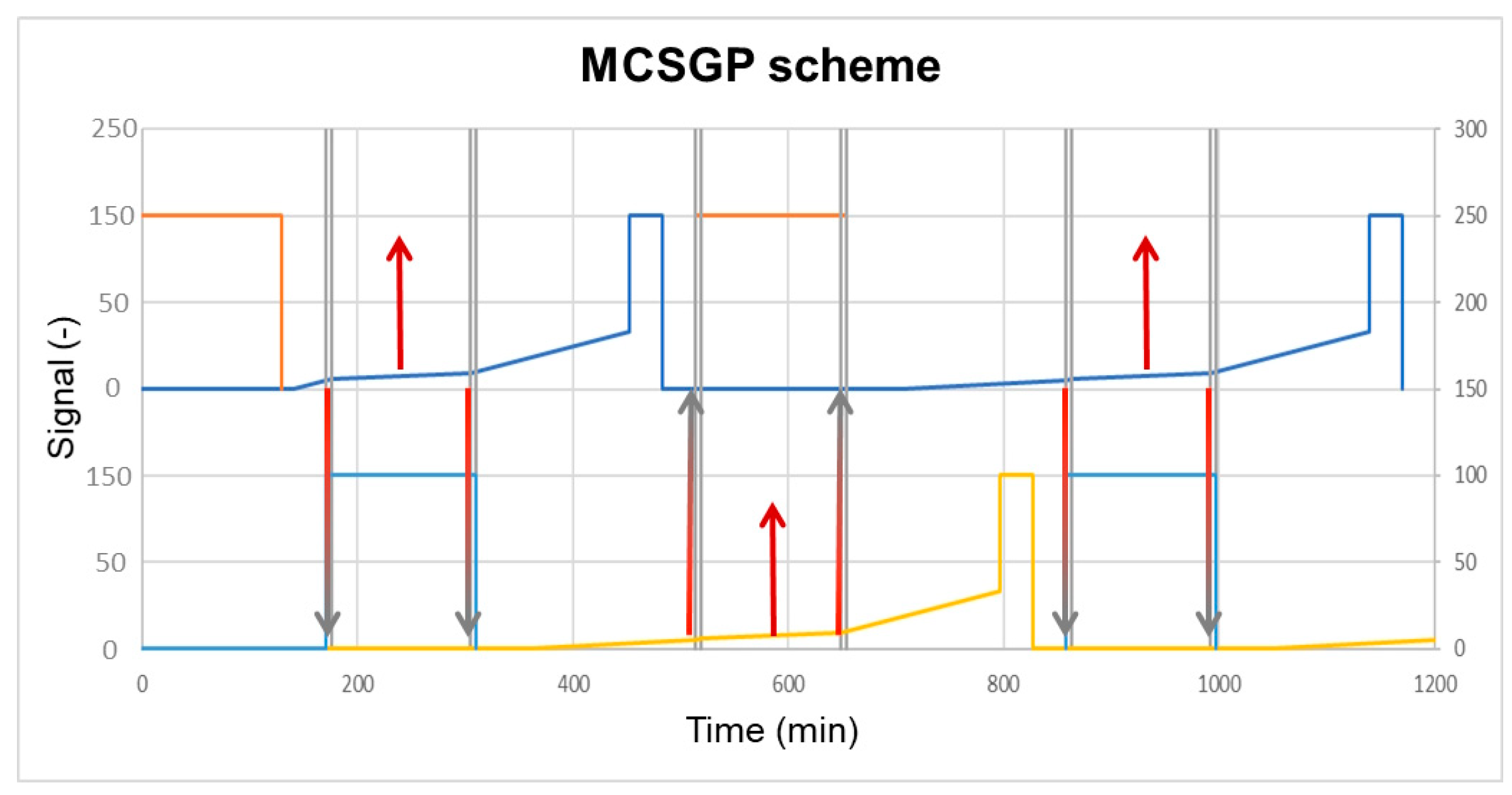
The established batch chromatography process model can be used to simulate various interconnections representing all types of continuous process variants.

4.1. MCSGP

The basic idea of the MCSGP process is a synchronized operation of two identical columns. While one is performing the gradient, the other is loaded with feed. The main benefit is high yield achieved through recycling. As depicted in Figure 4, the product peak is split up into three fractions. The fraction in the middle is the high purity product fraction (F2). The fractions before and afterwards contain an overlap of product and side components. These fractions are loaded to the other column before (F1) and after (F3) feed loading. Due to the gradient, inline dilution is necessary to dilute these fractions back to binding conditions. The MCSGP process ensures high yields without compromising purity.

However, the higher yield might come at the costs of productivity losses. As mentioned above, the two columns are synchronized. This forces one column to wait for the other. The loading of new feed on one column for example should take place during the exact same time as pure product elution from the other column. If both steps happen to take different amounts of time, one column has to wait for the other, or the flow rates have to be adjusted to slow down the faster process step. This is indicated in Figure 5.

Figure 5 shows an MCSGP scheduling where feed loading roughly takes 15 to 20 column volumes (CV). The gradient is roughly 10 CV with the product eluting in approximately 1.5 CV. Since fraction 1 should be loaded before feed and fraction 3 should be loaded after feed, the product elution must be slowed down. This is done by reducing the flow rate. As one can see in Figure 5, the gradient between two red to gray arrows is therefore very shallow. The gradient steepness in CV remains the same, but due to the low flow rate, it takes more time.

There is a similar issue for the regeneration and equilibration step of one column and the gradient start at the other. Regeneration and equilibration need to be finished before fraction 1 elutes; thus, again one column might need to wait for the other or adjust the flow rate.

For the process at hand, the column synchronization would lead to major delays almost doubling the process duration. Therefore, despite reaching over 99% yield during the first simulation studies, the decrease in productivity excluded MCSGP for further investigation.

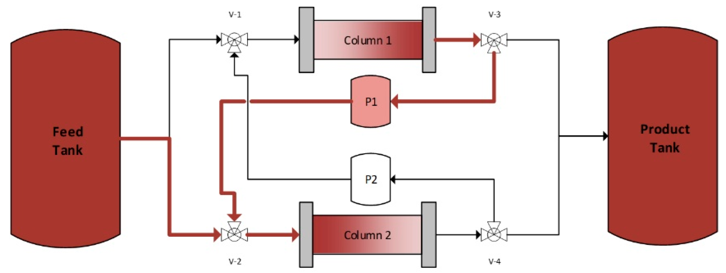
4.2. Continuous Twin Column Chromatography (CTCC)

To every problem there is a solution. The major advantage of the MCSGP process is high yield due to product recycling. The main disadvantage is longer process time due to column synchronization. Thus, the idea is to decouple both columns by storing the fractions F1 and F3 in additional tanks. This would additionally ease the necessary dilution.

First process simulations showed that purity is not influenced whether F1 and F3 are stored in two individual tanks (leading to a total of 4 tanks) or in one tank per column. Thus, the process scheme would look like Figure 6.

The use of tanks allows both columns to run at individual speeds. Only the total cycle time of both columns must be the same. In this case, loading took 1 CV longer than gradient, regeneration and equilibration. This was compensated for with 1 CV longer equilibration, leading to a theoretical productivity decrease of approximately 3%.

However, the overall yield could be increased drastically as shown in Figure 7:

As shown in Figure 1, the product peak has a sharp start and a tailing end. Thus, there is not much product in fraction 3. Hence, there are two reloading options. Reloading fraction 1 and 3 (A) or reloading fraction 1 only (B). Option A achieves higher yields but needs more time since fraction 2 elutes at a relatively high elution strength, thus needing more dilution before reloading and therefore adding more time to the loading phase.

The three different yields are explained as follows:

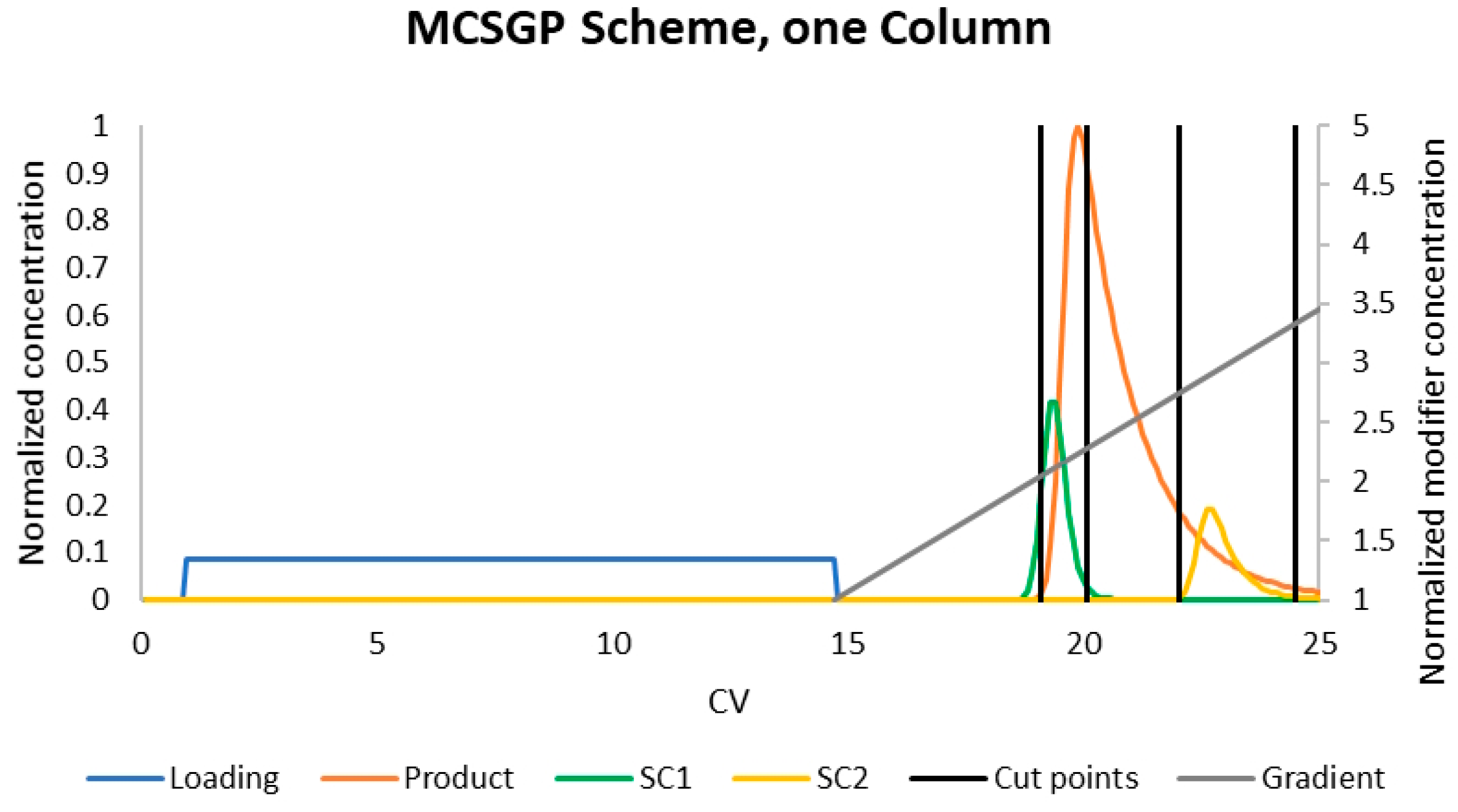
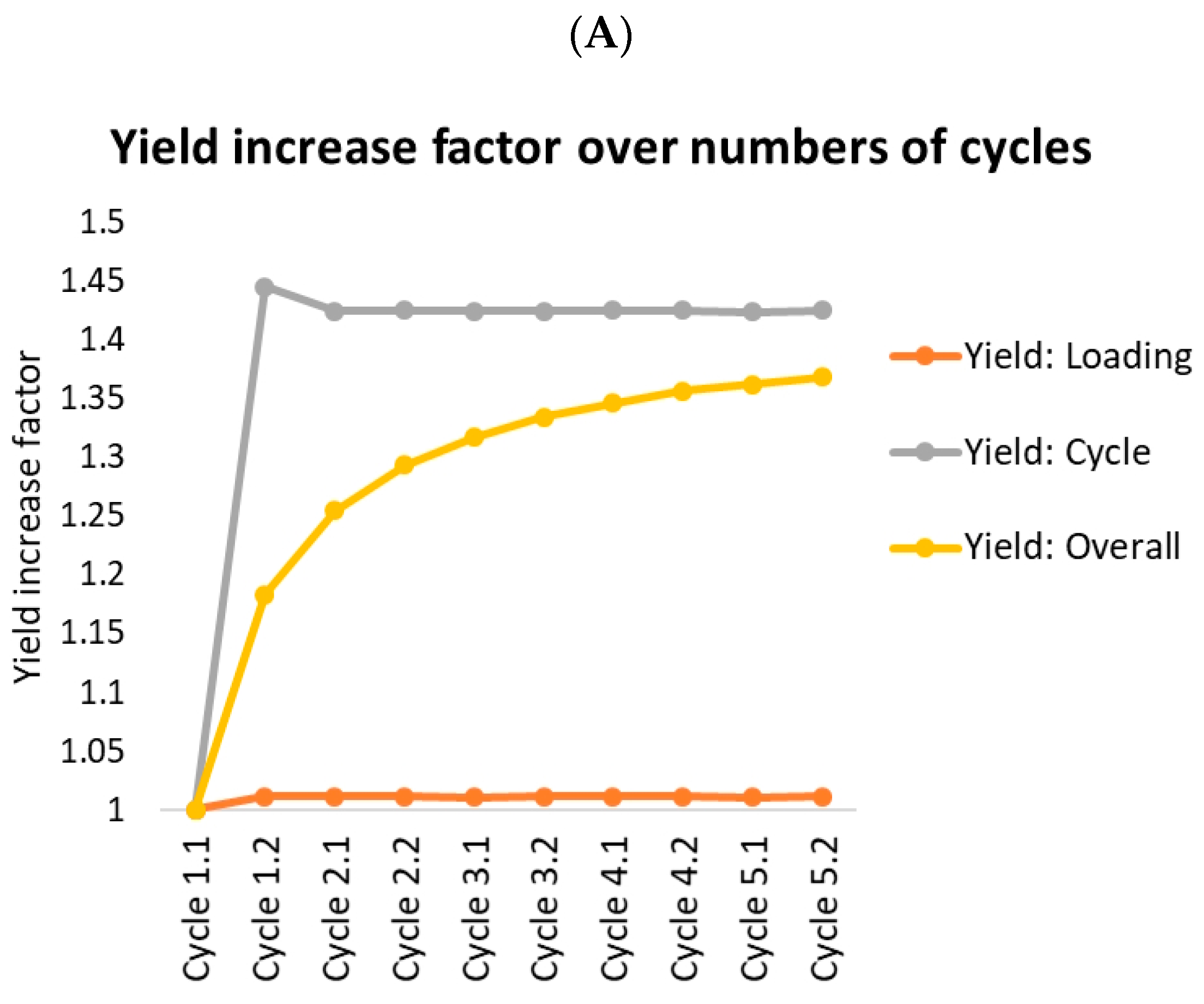
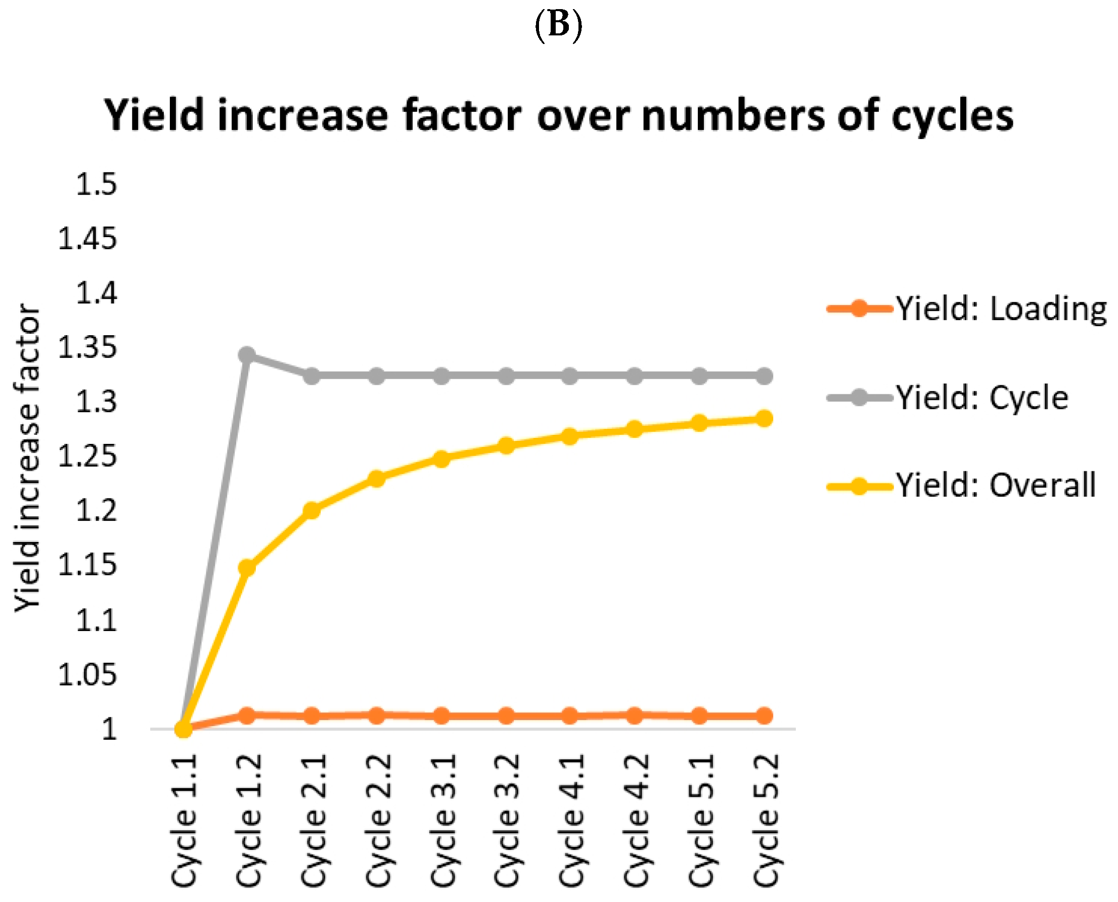
• Yield: Loading (orange lines) indicates the amount of product in product fraction compared to the overall amount loaded (feed plus reloading fractions) in this cycle. This should roughly resemble the batch yield.
• Yield: Cycle (gray) indicates the amount of product in product fraction compared to the amount of feed loaded in this cycle. Option A reaches 100% after the first cycle. There is no product lost at all. Option B loses 7% in fraction 3.
• Yield: Overall (yellow) indicates the overall amount of product gained compared to the overall amount of feed loaded. This starts at the batch yield and approaches the cycle yield, which it would reach after an infinite number of cycles. The gap between the cycle yield and the overall yield is caused by the amount of product stored in the fractions. Since this amount stays roughly the same, the yield loss caused by this becomes more and more unimportant compared to the overall amount of protein produced.

As shown in Figure 7, the CTCC process reaches 36.8% yield increase when both fractions are reloaded (A) and 28.5% if only fraction 1 is reprocessed (B).

However, option B takes less time. Therefore, the productivity increase is higher with 27.6% compared to 25.1%. The eluent consumption also decreases significantly. Option A has 23.6%, and option B has 20.2% less eluent consumption related to the amount of product. Due to slight changes in the cut points, specifically a narrower product fraction, the already very high purity of the corresponding batch process can be increased slightly.

4.3. Experimental Validation

The results of the simulation study were verified with pilot scale validation runs. These were performed on the multi-purpose chromatography prototype shown in Figure 8. The system contains six pumps, up to 60 valves and an array of different detectors and is, therefore, able to run a variety of continuous chromatography processes like MCSGP, PCC, SMB and more [41]. For this validation, only four pumps and two UV detectors were needed. Two Pumps are coupled to form a high-pressure gradient system; the other two pumps are used for feed loading and fraction reloading.

Two sets of long-term runs were done with 20 cycles each. An accumulation of side components was not observed, and the high initial peptide purity was maintained throughout the entire long-term runs. Simulations and experiments were in good agreement in terms of yield and productivity. The latter was found to be a little lower compared to the simulations (27.6%) leading to an overall productivity increase of 26.6% for the experimental validation runs compared to the experimental (and simulated) batch runs.

5. Conclusions

Starting from an existing preparative batch polishing step, a digital twin was successfully established, parametrized and validated. The model was then used to evaluate continuous chromatography options. MCSGP proved to be excellent in terms of purity and yield but with insufficient low productivity. An alternative Continuous Twin Column chromatography process (CTCC) was established that evades this drawback. These results of simulation studies were validated with two experimental long runs on a multi-purpose prototype. The already high purity of the batch step could be improved slightly. Yield and productivity, however, were increased significantly by 27.6% and 26.6%, respectively. Additionally, eluent consumption decreased by 20.2%.

References

1. Carta, G.; Jungbauer, A. Protein Chromatography: Process Development and Scale-Up; Wiley-VCH: Weinheim, Germany, 2010; ISBN 978-3-527-31819-3. [Google Scholar]
2. Scopes, R.K. Protein Purification: Principles and Practice, 3rd ed.; Springer: New York, NY, USA, 1994; ISBN 978-1-4757-2333-5. [Google Scholar]
3. Subramanian, G. (Ed.) Biopharmaceutical Production Technology; Wiley-VCH: Weinheim, Germany, 2012; ISBN 9783527653096. [Google Scholar]
4. Kornecki, M.; Mestmäcker, F.; Zobel-Roos, S.; Heikaus de Figueiredo, L.; Schlüter, H.; Strube, J. Host Cell Proteins in Biologics Manufacturing: The Good, the Bad, and the Ugly. Antibodies 2017, 6, 13. [Google Scholar] [CrossRef]
5. Gronemeyer, P.; Strube, J. Purification of Antibodies and their Fragments by ATPE and Precipitation: One Step towards a Chromatography-Free Manufacturing Process. Chem. Ing. Tech. 2015, 87, 1057–1058. [Google Scholar] [CrossRef]
6. Subramanian, G. (Ed.) Continuous Biomanufacturing: Innovative Technologies and Methods; Wiley-VCH: Weinheim, Germany, 2018; ISBN 9783527699902. [Google Scholar]
7. Strube, J. Technische Chromatographie: Auslegung, Optimierung, Betrieb und Wirtschaftlichkeit; Als Ms. gedr; Univ., Habil.-Schr.: Dortmund, Germany; Shaker: Aachen, Germany, 2000; ISBN 3826568974. [Google Scholar]
8. Rodrigues, A. Simulated Moving Bed Technology: Principles, Design and Process Applications; Elsevier Science: Burlington, ON, Canada, 2015; ISBN 9780128020241. [Google Scholar]
9. Kaspereit, M.; Seidel-Morgenstern, A. Auslegung der Regenerationszonen des SMB-Verfahrens. Chem. Ing. Tech. 2002, 74, 591–592. [Google Scholar] [CrossRef]
10. Mazzotti, M. Equilibrium theory based design of simulated moving bed processes for a generalized Langmuir isotherm. J. Chromatogr. A 2006, 1126, 311–322. [Google Scholar] [CrossRef]
11. Wellhoefer, M.; Sprinzl, W.; Hahn, R.; Jungbauer, A. Continuous processing of recombinant proteins: Integration of refolding and purification using simulated moving bed size-exclusion chromatography with buffer recycling. J. Chromatogr. A 2014, 1337, 48–56. [Google Scholar] [CrossRef] [PubMed]
12. Aumann, L.; Morbidelli, M. A continuous multicolumn countercurrent solvent gradient purification (MCSGP) process. Biotechnol. Bioeng. 2007, 98, 1043–1055. [Google Scholar] [CrossRef]
13. de Luca, C.; Lievore, G.; Bozza, D.; Buratti, A.; Cavazzini, A.; Ricci, A.; Macis, M.; Cabri, W.; Felletti, S.; Catani, M. Downstream Processing of Therapeutic Peptides by Means of Preparative Liquid Chromatography. Molecules 2021, 26, 4688. [Google Scholar] [CrossRef]
14. de Luca, C.; Felletti, S.; Lievore, G.; Buratti, A.; Vogg, S.; Morbidelli, M.; Cavazzini, A.; Catani, M.; Macis, M.; Ricci, A.; et al. From batch to continuous chromatographic purification of a therapeutic peptide through multicolumn countercurrent solvent gradient purification. J. Chromatogr. A 2020, 1625, 461304. [Google Scholar] [CrossRef]
15. Aumann, L.; Stroehlein, G.; Muller-Spath, T.; Schenkel, B.; Morbidelli, M. Protein Peptide Purification using the Multicolumn Countercurrent Solvent Gradient Purification (MCSGP) Process. BioPharm Int. 2009, 22. [Google Scholar]
16. Zobel-Roos, S.; Mouellef, M.; Ditz, R.; Strube, J. Distinct and Quantitative Validation Method for Predictive Process Modelling in Preparative Chromatography of Synthetic and Bio-Based Feed Mixtures Following a Quality-by-Design (QbD) Approach. Processes 2019, 7, 580. [Google Scholar] [CrossRef]
17. Kaczmarski, K.; Cavazzini, A.; Szabelski, P.; Zhou, D.; Liu, X.; Guiochon, G. Application of the general rate model and the generalized Maxwell–Stefan equation to the study of the mass transfer kinetics of a pair of enantiomers. J. Chromatogr. A 2002, 962, 57–67. [Google Scholar] [CrossRef] [PubMed]
18. Kaczmarski, K.; Gubernak, M.; Zhou, D.; Guiochon, G. Application of the general rate model with the Maxwell–Stefan equations for the prediction of the band profiles of the 1-indanol enantiomers. Chem. Eng. Sci. 2003, 58, 2325–2338. [Google Scholar] [CrossRef]
19. Guiochon, G.; Felinger, A.; Shirazi, D.G.; Katti, A.M. Fundamentals of Preparative and Nonlinear Chromatography, 2nd ed.; Elsevier Academic Press: Amsterdam, The Netherlands, 2006. [Google Scholar]
20. Zobel-Roos, S. Entwicklung, Modellierung und Validierung von Integrierten Kontinuierlichen Gegenstrom-Chromatographie-Prozessen; 1. Auflage; Shaker: Herzogenrath, Germany, 2018; ISBN 3844061878. [Google Scholar]
21. Felinger, A.; Guiochon, G. Comparison of the Kinetic Models of Linear Chromatography. Chromatographia 2004, 60, S175–S180. [Google Scholar] [CrossRef]
22. Piątkowski, W.; Antos, D.; Kaczmarski, K. Modeling of preparative chromatography processes with slow intraparticle mass transport kinetics. J. Chromatogr. A 2003, 988, 219–231. [Google Scholar] [CrossRef]
23. Seidel-Morgenstern, A. Experimental determination of single solute and competitive adsorption isotherms. J. Chromatogr. A 2004, 1037, 255–272. [Google Scholar] [CrossRef]
24. Asnin, L. Adsorption models in chiral chromatography. J. Chromatogr. A 2012, 1269, 3–25. [Google Scholar] [CrossRef] [PubMed]
25. Blümel, C.; Kniep, H.; Seidel-Morgenstern, A. Measuring adsorption isotherms using a closed-loop perturbation method to minimize sample consumption. In Proceedings of the 6th International Conference of Fundamentals of Adsorption—FOA 6, Presqu’ile de Giens, France, 23–27 May 1998; Elsevier: Amsterdam, The Netherlands, 1998; pp. 449–454. [Google Scholar]
26. Cavazzini, A.; Felinger, A.; Guiochon, G. Comparison between adsorption isotherm determination techniques and overloaded band profiles on four batches of monolithic columns. J. Chromatogr. A 2003, 1012, 139–149. [Google Scholar] [CrossRef] [PubMed]
27. Ching, C.B.; Chu, K.H.; Ruthven, D.M. A study of multicomponent adsorption equilibria by liquid chromatography. AIChE J. 1990, 36, 275–281. [Google Scholar] [CrossRef]
28. Gamba, G.; Rota, R.; Storti, G.; Carra, S.; Morbidelli, M. Absorbed solution theory models for multicomponent adsorption equilibria. AIChE J. 1989, 35, 959–966. [Google Scholar] [CrossRef]
29. Hu, X.; Do, D.D. Comparing various multicomponent adsorption equilibrium models. AIChE J. 1995, 41, 1585–1592. [Google Scholar] [CrossRef]
30. Heinonen, J.; Rubiera Landa, H.O.; Sainio, T.; Seidel-Morgenstern, A. Use of Adsorbed Solution theory to model competitive and co-operative sorption on elastic ion exchange resins. Sep. Purif. Technol. 2012, 95, 235–247. [Google Scholar] [CrossRef]
31. Emerton, D.A. Profitability in the Biosimilars Market: Can You Translate Scientific Excellence into a Healthy Commercial Return? BioProcess Int. 2013, 11, 6–23. [Google Scholar]
32. Erto, A.; Lancia, A.; Musmarra, D. A modelling analysis of PCE/TCE mixture adsorption based on Ideal Adsorbed Solution Theory. Sep. Purif. Technol. 2011, 80, 140–147. [Google Scholar] [CrossRef]
33. Myers, A.L.; Prausnitz, J.M. Thermodynamics of mixed-gas adsorption. AIChE J. 1965, 11, 121–127. [Google Scholar] [CrossRef]
34. Costa, E.; Calleja, G.; Marron, C.; Jimenez, A.; Pau, J. Equilibrium adsorption of methane, ethane, ethylene, and propylene and their mixtures on activated carbon. J. Chem. Eng. Data 1989, 34, 156–160. [Google Scholar] [CrossRef]
35. Brooks, C.A.; Cramer, S.M. Steric mass-action ion exchange: Displacement profiles and induced salt gradients. AIChE J. 1992, 38, 1969–1978. [Google Scholar] [CrossRef]
36. Langmuir, I. The adsorption of gases on plane surfaces of glass, mica and platinum. J. Am. Chem. Soc. 1918, 40, 1361–1403. [Google Scholar] [CrossRef]
37. DePhillips, P.; Lenhoff, A.M. Pore size distributions of cation-exchange adsorbents determined by inverse size-exclusion chromatography. J. Chromatogr. A 2000, 883, 39–54. [Google Scholar] [CrossRef]
38. Goto, M.; McCoy, B.J. Inverse size-exclusion chromatography for distributed pore and solute sizes. Chem. Eng. Sci. 2000, 55, 723–732. [Google Scholar] [CrossRef]
39. Levenspiel, O. Chemical Reaction Engineering, 3rd ed.; Wiley: New York, NY, USA, 1999; ISBN 9780471254249. [Google Scholar]
40. Jacobson, J.M.; Frenz, J.H.; Horvath, C.G. Measurement of competitive adsorption isotherms by frontal chromatography. Ind. Eng. Chem. Res. 1987, 26, 43–50. [Google Scholar] [CrossRef]
41. Strube, J.; Zobel-Roos, S. Preparative Chromatography for (Bio)Pharmaceuticals: Digital Multi-Purpose Plants for Fast and Flexible Process Solutions. Available online: https://analyticalscience.wiley.com/do/10.1002/was.00080322 (accessed on 15 March 2022).
Figure 1. Batch chromatogram of the peptide polishing step. The solid blue line is the chromatogram at 280 nm measured with a diode array detector (DAD), assigned to the right axis. The left concentration axis is zoomed in to show the side components (SC), which are represented with dots.
Processes 11 01401 g001
Figure 2. Comparison between measurements (dotted lines) and simulations (solid lines) for two different volumetric flows (0.33 CV/min, yellow; 0.66 CV/min, green). Time scale and volumetric flow are normalized to CV and CV/min, respectively.
Processes 11 01401 g002
Figure 3. Comparison between measurements (dotted lines) and simulations (solid lines) for a batch chromatography run. The target component is given in orange. Side components in blue. The gradient is shown with a green line.
Processes 11 01401 g003
Figure 4. Chromatogram of a batch run with relevant cut points (black lines) for MCSGP operation.
Processes 11 01401 g004
Figure 5. MCSGP scheduling for column 1 (upper) and 2 (lower). Gray lines indicate fraction cut points. The color shifting arrows (red to gray) indicate the transfer of fraction 1 or 3 from one column to the other. Pure red arrows indicate pure product elution. Orange (above) and blue (below) lines indicate feed loading.
Processes 11 01401 g005
Figure 6. Process scheme for the CTCC process.
Processes 11 01401 g006
Figure 7. Purity (blue line) and yield for (A) reloading of fraction 1 and 3 and (B) reloading fraction 1 only.
Processes 11 01401 g007aProcesses 11 01401 g007b
Figure 8. Multi-purpose continuous chromatography prototype.
Processes 11 01401 g008
Disclaimer/Publisher’s Note: The statements, opinions and data contained in all publications are solely those of the individual author(s) and contributor(s) and not of MDPI and/or the editor(s). MDPI and/or the editor(s) disclaim responsibility for any injury to people or property resulting from any ideas, methods, instructions or products referred to in the content.