Separation of Ternary System 1,2-Ethanediol + 1,3-Propanediol + 1,4-Butanediol by Liquid-Only Transfer Dividing Wall Column

Abstract

This study focuses on separating a mixture consisting of 1,2-ethanediol (1,2-ED), 1,3-propanediol (1,3-PD), and 1,4-butanediol (1,4-BD). Vapor–liquid equilibrium (VLE) data for 1,2-ED + 1,4-BD and 1,3-PD + 1,4-BD are determined at 101.3 kPa using a modified Rose equilibrium still. The consistency of the VLE data is checked with both Redlich–Kister and Fredenslund tests. The VLE data are fitted by the Wilson, NRTL, and UNIQUAC activity coefficient models. All three models can effectively correlate the VLE data. Then, the separation of the mixture is designed with the NRTL model and its correlated binary interaction parameters. A liquid-only transfer dividing wall column (LDWC) is investigated on the basis of a direct conventional distillation sequence (DCDS). For a fair comparison, both DCDS and LDWC are optimized to minimize total annual cost using sequential iterative optimization procedures. After optimization, LDWC exhibits a 16.87% reduction in total annual cost, while cooling and heating utility consumptions are reduced by 28.40% and 19.24% compared to DCDS.

1. Introduction

Diols including 1,2-ethanediol (1,2-ED), 1,3-propanediol (1,3-PD), and 1,4-butanediol (1,4-BD) can be used as solvents, antifreeze, pharmaceutical synthesis, polyester intermediates, etc. [1]. They can be obtained through chemical synthesis or catalytic hydrocracking of sorbitol derived from bioconversion processes [2]. Separation and purification are the keys to their industrial application. Distillation, as the most widely applied separation technology [3], is considered in this article. As conventional distillation column normally consumes a large amount of energy [4,5,6,7], it is promising to find an alternative column configuration with lower energy consumption.

Dividing wall column (DWC) involving a vertical partition wall proposed by R.O. Wright can be one of the alternative column configurations [8]. It reduces the internal re-mixing of the feed stream and side-draw product [9], reducing energy consumption compared to the conventional distillation column. In addition, it saves capital costs by reducing one condenser and reboiler by integrating the main column and prefractionator into a single shell. Much research has been done on the DWC for ternary mixture separation. Kaibel [8] studied the performance of DWC to separate a mixture of n-octane, n-heptane, and n-hexane under an equimolar fraction feed. It showed that DWC can reduce about 20% of the energy consumption compared with direct conventional distillation sequence (DCDS). Kolbe and Wenzel [10] applied the DWC to petrochemical cuts and calculated its capital cost. Approximately 20% of capital cost can be saved, along with higher capacity compared to DCDS. Ling et al. [11] investigated the controllability of the benzene, toluene, and o-xylene DWC through a four-column equivalent model. It demonstrated that product purity can be controlled by manipulating reflux ratio, side-product flow, liquid split, and ratio reboiler duty with a tiny purity deviation. However, only about 200 DWCs have been built globally [12]. Effectively controlling the vapor split ratio [13], which substantially impacts product purity, capital cost, and energy consumption, is one of the DWC application’s constraints.

To eliminate the vapor split ratio, Agrawal proposed a new alternative configuration named the liquid-only transfer DWC (LDWC) [13], shown in Figure 1. Ramapriya and Agrawal [13] have demonstrated that LDWC is equivalent to DWC through physical reasoning. Cui et al. [14] investigated ten different liquid-only transfer topologies that could separate the equimolar mixture of benzene, toluene, and m-xylene. These topologies included DCDS and LDWC. The simulation results showed that LDWC could save economic and energy consumption compared to the other nine topologies. Based on the static state study, Cui et al. [15] investigated LDWC dynamic control performance for the ternary mixture separation. The product purity could be maintained using five temperature controllers with an additional internal composition controller when handling ±20% disturbance in feed flow or composition. Furthermore, Zhang et al. [16] focused on the dynamic control of LDWC for the separation of an equimolar quaternary mixture. Their work showed that LDWC can be easily controlled well only using temperature controllers facing ±15% disturbance. LDWC provides a new path for DWC’s application. So, it is used to separate the diols in this study.

Vapor–liquid equilibrium (VLE) data are the foundation for distillation separation. Our previous work determined VLE data for the system of 1,2-ED and 1,3-PD at 101.3 kPa [17]. The VLE data for the system 1,2-PD + 1,4-BD at 10 kPa, 20 kPa, and 40 kPa have been measured by Yang et al. [18]. However, VLE data for the two binary mixtures 1,2-ED + 1,4-BD and 1,3-PD + 1,4-BD at 101.3 kPa were not found in the NIST Thermodata Engine. Thus, the VLE data for these two binary mixtures at 101.3 kPa are measured and then regressed by activity coefficient models including Wilson [19], NRTL [20], and UNIQUAC [21] via Aspen Plus V11. It is unclear that the performance of the LDWC is used for the diols mixtures separation. Therefore, the LDWC for the diols mixtures separation is simulated using Aspen Plus based on the correlated binary interaction parameters. And DCDS, as illustrated in Figure 2, is carried out as the base case. For a fair comparison, sequential iterative optimization procedures were used to minimize the total annual cost of each configuration. This study can promote the industrial application of LDWC for diols separation.

2. Experimental and Process Modeling

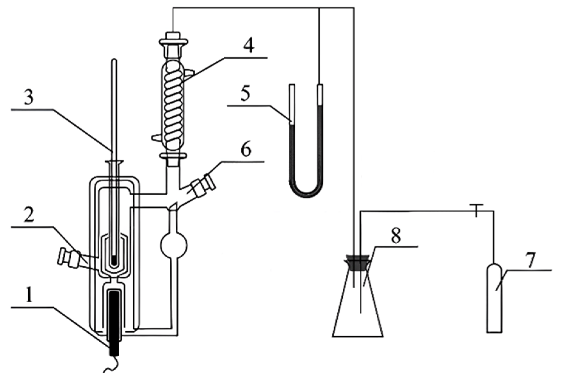
2.1. Materials

1,2-ED, 1,3-PD, and 1,4-BD were the chemical reagents utilized in this investigation. Their purity is checked by gas chromatography (Zhejiang Fuli Instruments, GC-9790plus, Taizhou, China). The detailed information, including density and boiling point, is summarized in

Table 1. Details of chemical reagents ^a.

Component	CAS	Supplier	Purity (wt %)	Density (g·cm−3)		Boiling Point (K)		Analysis Method
				Exp c	Lit d	Exp e	Lit f
1,2-ED	107-21-1	Sinopharm, Beijing, China	≥99.0	1112	1110 [22]	470.25	470.45 [23]	GC b
1,3-PD	504-63-2	Accela, Shanghai, China	≥98.0	1053	1050 [24]	487.35	487.55 [24]
1,4-BD	110-63-4	Sinopharm, Beijing, China	≥99.0	1012	1016.9 [25]	501.05	501.15 [25]

^a Standard uncertainties of T and p are u(T) = 0.1 K and u(p) = 0.1 kPa, respectively. ^b Gas chromatography. ^d, ^f Reported in literature. ^c Experiments conducted at 293.75 K. ^e Experiments performed at 101.3 kPa.

. It is important to note that these chemicals are used without further treatment.

2.2. Methods

A modified Rose equilibrium still, depicted in Figure 3, was employed to determine VLE data in this study. Our previous work [26,27] demonstrated the reliability of the apparatus. The apparatus facilitates the establishment of equilibrium by continuous recirculation of both the vapor and liquid phases. For each experiment, 40 mL of the liquid mixture was added to the modified Rose still. Then, the heating rate was tuned to maintain a vapor phase condensation rate of approximately 60 drops per minute. After the temperatures of the vapor and liquid phases were maintained for more than 60 min, equilibrium was reached. Then, both liquid and condensed vapor were sampled for subsequent analysis.

Two precision mercury thermometers were used to measure the equilibrium temperature. These two thermometers, respectively, have a scale from 150 °C to 200 °C and 200 °C to 250 °C, with a division value of 0.1 °C. Nitrogen was continually added from the nitrogen cylinder to control the pressure. The standard uncertainties of T and p were 0.1 K and 0.1 kPa, respectively. It is noted that the conversion from Celsius to Kelvin is obtained by adding 273.15 and then rounding up.

Gas chromatography (Zhejiang Fuli Instruments, GC-9790plus) with a flame ionization detector (FID) and a capillary column (PEG-20M, 30 m × 0.32 mm × 0.5 μm) was used to examine each sample. A total of 0.1 μL of the sample was injected each time. The carrier gas was high-purity nitrogen (99.999%, wt) at a flow rate of 30 mL/min. Both the detector and the injector had a temperature of 523.15 K. The temperature of the column was programmed in the following manner: initially, it was maintained at a temperature of 373.15 K for a duration of 4 min. Subsequently, the temperature was raised to 503.15 K at a rate of 5 K per minute and held at this temperature for a period of 3 min. To assure accuracy, each sample was measured at least three times.

2.3. Simulation

The simulation employed a mixture consisting of 1,2-ED, 1,3-PD, and 1,4-BD. The feed was introduced at a flow rate of 100 kmol/h, featuring a uniform distribution of mole fractions, representing a challenging separation scenario. All products’ target concentration was assumed to be 99.0 mol%. The operational pressure remained consistent with the experimental conditions.

RadFrac module can be used for rigorous calculation for conventional distillation columns. However, no built-in module is available for LDWC in Aspen Plus. When the heat transfer on both sides of the partition is ignored, the equivalent model of LDWC can be derived by the RadFrac modules [15,16], as illustrated in Figure 4.

2.4. Optimization

The simplicity of sequential iterative optimization procedures has contributed to their extensive application in the optimization of diverse distillation systems [28,29,30]. Therefore, two sequential iterative optimization procedures are proposed to optimize DCDS and LDWC, as illustrated in Figure 5 and Figure 6, respectively. Herein, the primary objective is to minimize the total annual cost (TAC) because it simultaneously considers operating cost and capital cost. TAC in this study can be calculated by the Douglas equations [31], which are provided in Appendix A.

As shown in Figure 2, DCDS has four independent discrete design variables and four independent continuous design variables. The discrete design variables include the total theoretical stages of C1 and C2 (N_C1, N_C2) and the feed stage locations of C1 and C2 (NF_C1, NF_C2). The continuous design variables include the distillation flow rates of C1 and C2 (DF_C1, DF_C2) and the reflux ratios of C1 and C2 (RR_C1, RR_C2). The sequence iterative optimization procedure of DCDS can be manipulated as follows:

(1)

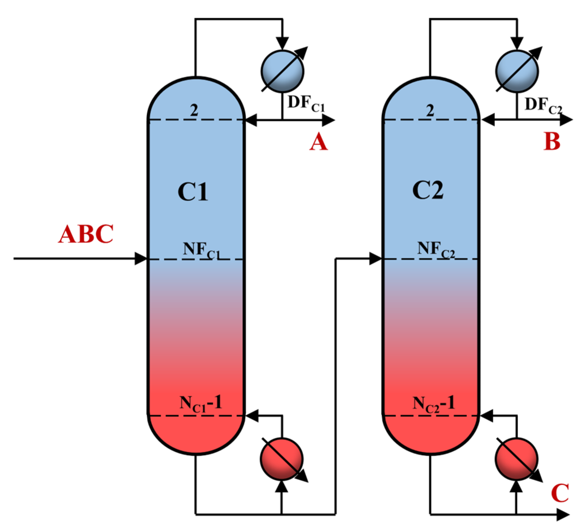
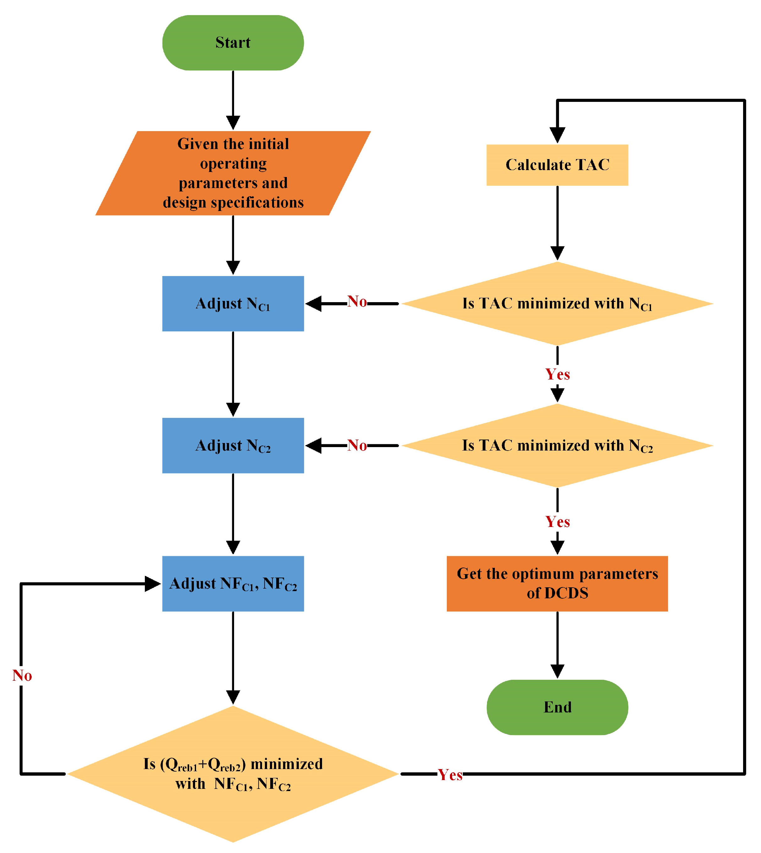
Specify the initial operation parameters and use Design specifications and vary modules in simulation to maintain target purity. Herein, target purity is achieved by manipulating DF_C1, DF_C2, RR_C1, and RR_C2 using these two modules.

(2)

Adjust NF_C1 and NF_C2 to minimize the total heat duty (Q_reb1 + Q_reb2).

(3)

If the TAC is minimized with N_C1, obtain the optimum N_C1; if not, adjust N_C1 and go back to step 2.

(4)

If the TAC is minimized with N_C2, obtain the optimum N_C2; if not, adjust N_C2 and go back to step 2.

(5)

Obtain the optimum parameters of DCDS.

LDWC, shown in Figure 1, involved eight independent discrete design variables and seven independent continuous design variables. The eight discrete variables are the total theoretical stages of CL and CR (N_CL, N_CR), the feed stages location of CL and CR (NF_LDWC, N_{AB_IN}, N_{BC_IN}), and the side-draw stages location of CL and CR (N_{AB_OUT}, N_{BC_OUT}, N_B). The seven continuous variables are the distillation flow rates and reflux ratios of CL and CR section (DF_CL, DF_CR, RR_CL, RR_CR), the flow rates of liquid-only transfer streams AB and BC(F_AB, F_BC), and the side-draw stage flow rate (F_B). In the sequence iterative optimization procedure of LDWC, the optimum parameters can be obtained as follows:

(1)

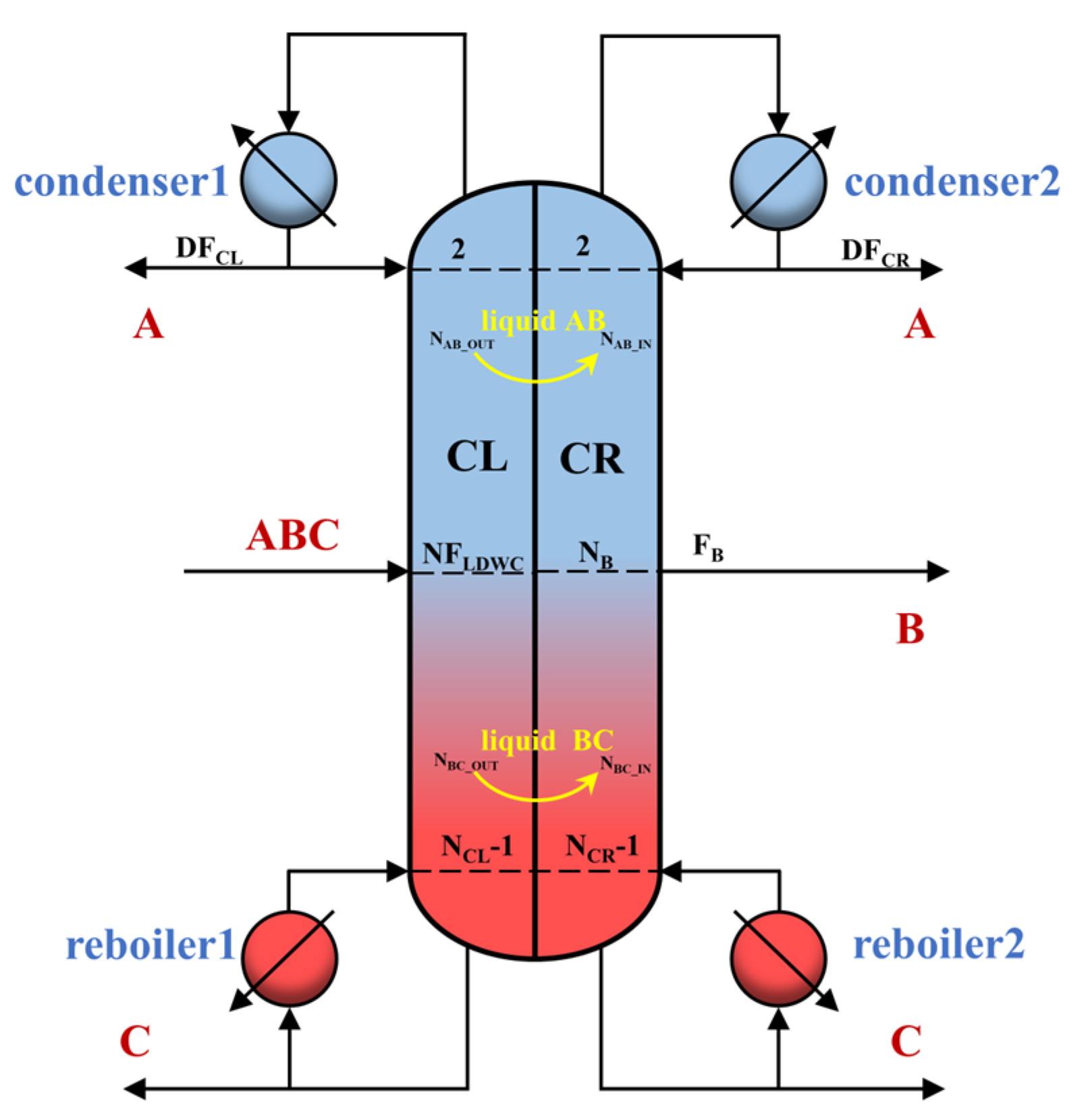
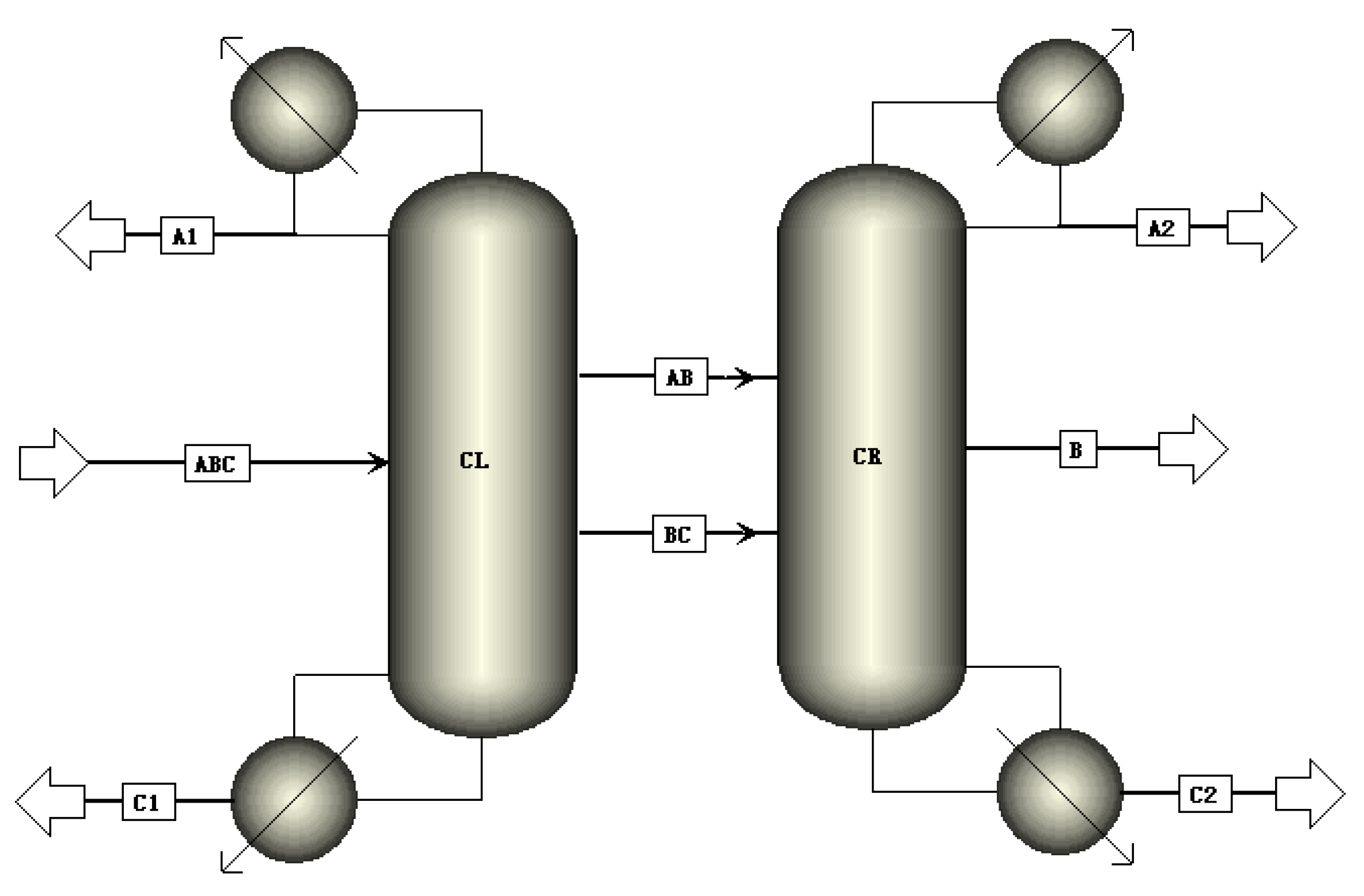
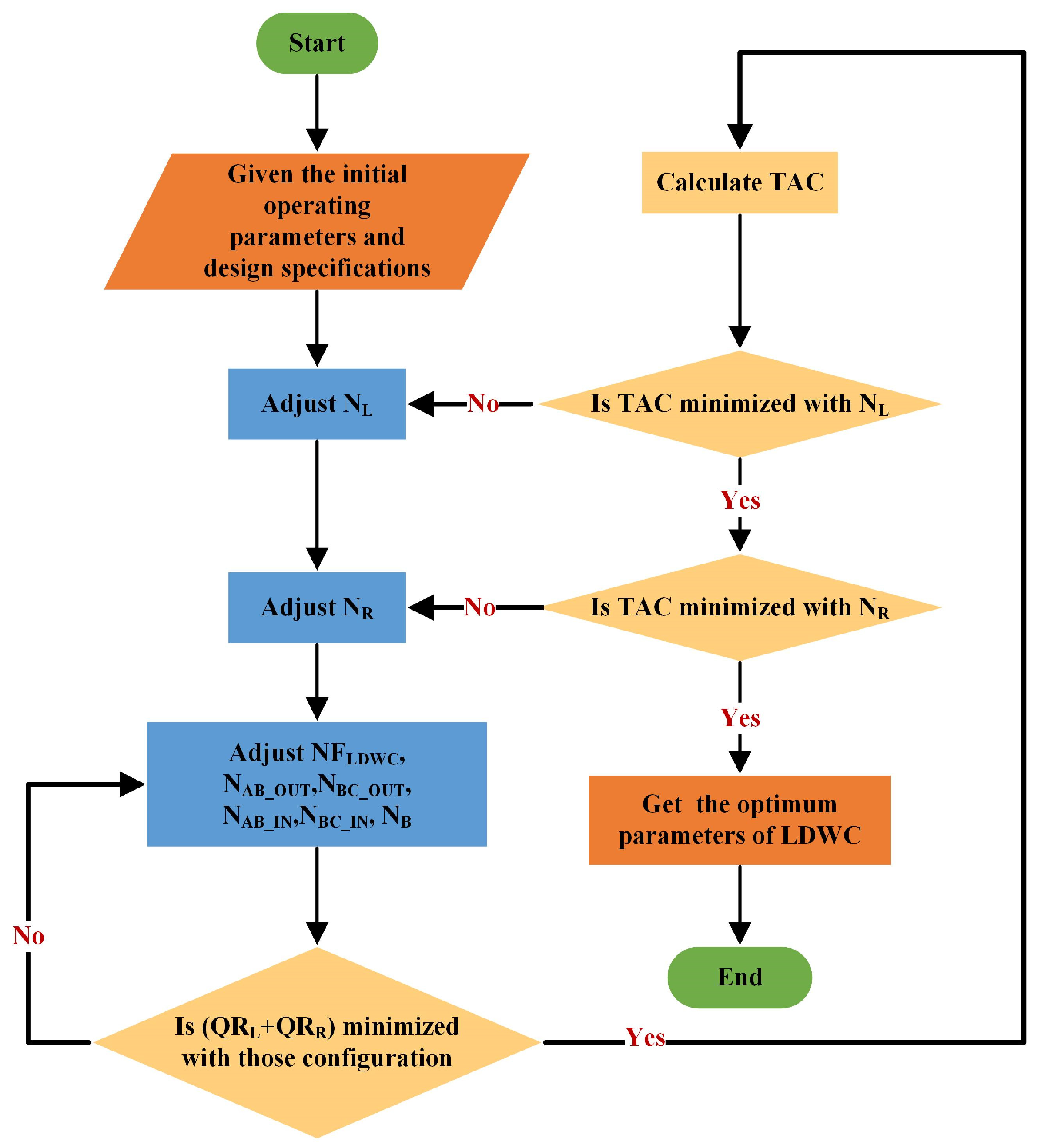
Specify the initial operation parameters and use design specifications in Aspen Plus to maintain target purity. Herein, target purity is obtained by manipulating DF_CL, DF_CR, RR_CL, RR_CR, and F_B using these two modules.

(2)

Adjust NF_LDWC, N_{AB_OUT}, N_{BC_OUT}, N_{AB_IN}, N_{BC_IN}, and N_B to minimize the total heat duty (QR_L + QR_R).

(3)

If the TAC is minimized with N_L, get the optimum N_L; if not, adjust N_L and go back to step 2.

(4)

If the TAC is minimized with N_R, get the optimum N_R; if not, adjust N_R and go back to step 2.

(5)

Get the optimum parameters of DCDS.

In addition, the related discrete and continuous design variables for DCDS and LDWC are marked in Figure 1 and Figure 2.

3. Results and Discussion

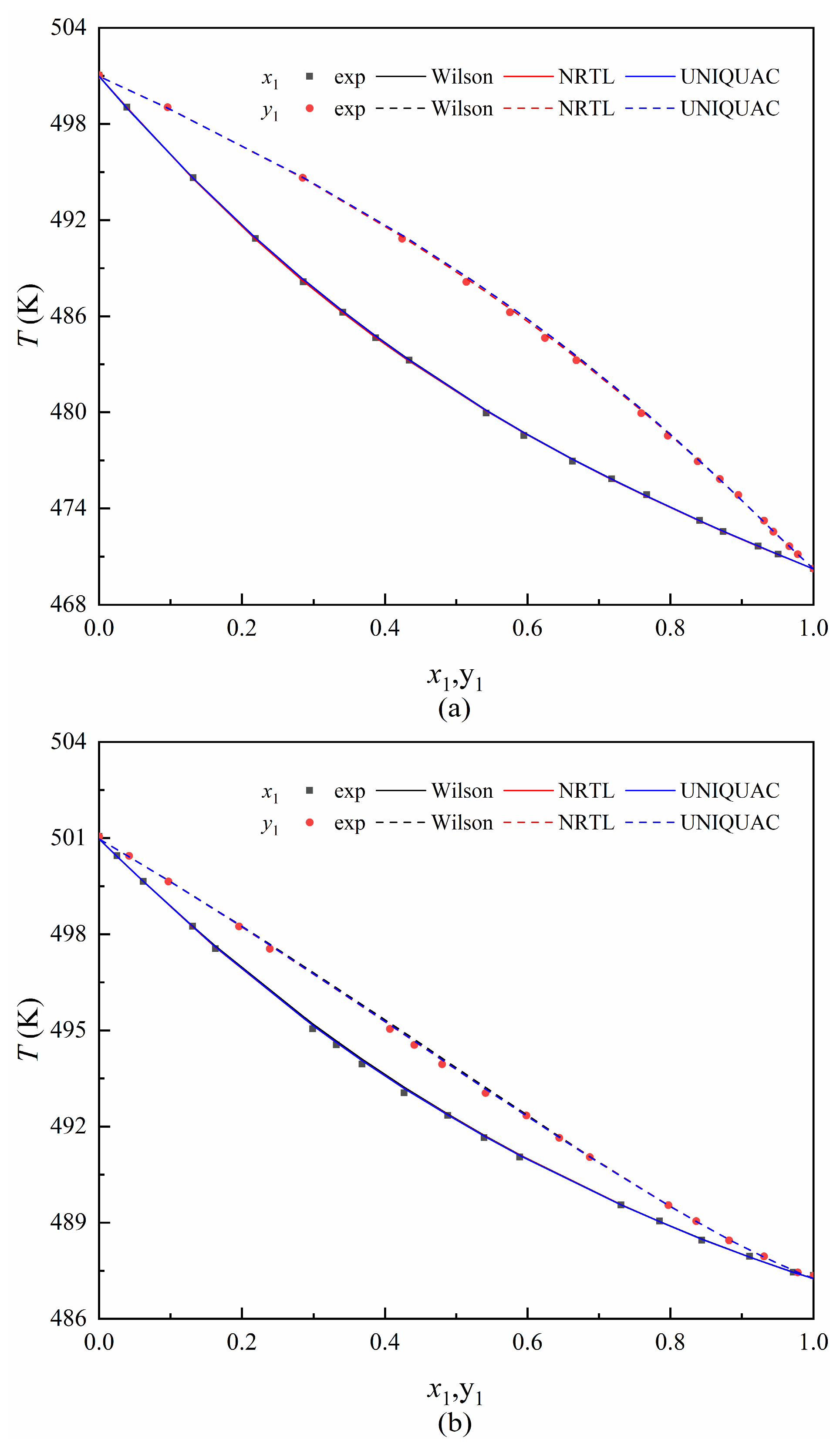
3.1. Phase Equilibrium Data

The VLE data of 1,2-ED (1) + 1,4-BD (2) and 1,3-PD (1) + 1,4-BD (2) at 101.3 kPa are listed in Appendix B. The vapor and liquid phase equilibrium relationship is expressed as Equation (1).

$${\phi }_i^{v}p{y}_i={\gamma }_i{x}_i{p}_i^s{\phi }_i^s\exp \left(\frac{V_i^L\left(p-p_i^s\right)}{RT}\right)$$

(1)

where T and p are the temperature and pressure of the systems, respectively; x_i and y_i are mole fractions of component i in the liquid and vapor phases, respectively; γ_i is the activity coefficient of component i in the liquid phase; R is the gas constant; and V_i^L is the liquid mole volume of pure component i.

Meanwhile, φ_i^v and φ_i^s represent the fugacity coefficient of component i in the vapor and saturated vapor phases, respectively. The vapor phase can be treated as an ideal gas at 101.3 kPa [32], which means that the last term on the right of Equation (1), φ_i^v_, and φ_i^s can be assumed to be 1. Thus, the VLE relationship can be simplified as Equation (2).

$$p{y}_i={\gamma }_i{x}_i{p}_i^s$$

(2)

where p_i^s is the saturated vapor pressure of pure component i. It can be calculated by Extended Antoine Equation (3).

$$\ln (p_i^s)=C_{1i}+\frac{C_{2i}}{T+C_{3i}}+C_{4i}T+C_{5i}\ln (T)+C_{6i}{T}^{C_{7i}} \mathrm{for} C_{8i} \le T \le C_{9i}$$

(3)

where the constants C_1i–C_9i are Extended Antoine Coefficients for component i, which are listed in

Table 2. Antoine coefficients for vapor pressure ^a.

Component	C1i	C2i	C3i	C4i	C5i	C6i	C7i	C8i	C9i
1,2-ED b	84.09	10411	0	0	8.1976	1.65 × 10−18	6	260.15	720
1,3-PD b	115.58	−11732	0	0	−13.174	6.55 × 10−6	2	246.45	724
1,4-BD b	105.76	−12811	0	0	−11.069	9.44 × 10−18	6	293.05	667

^a from Aspen Plus. ^b T/K, p/Pa.

.

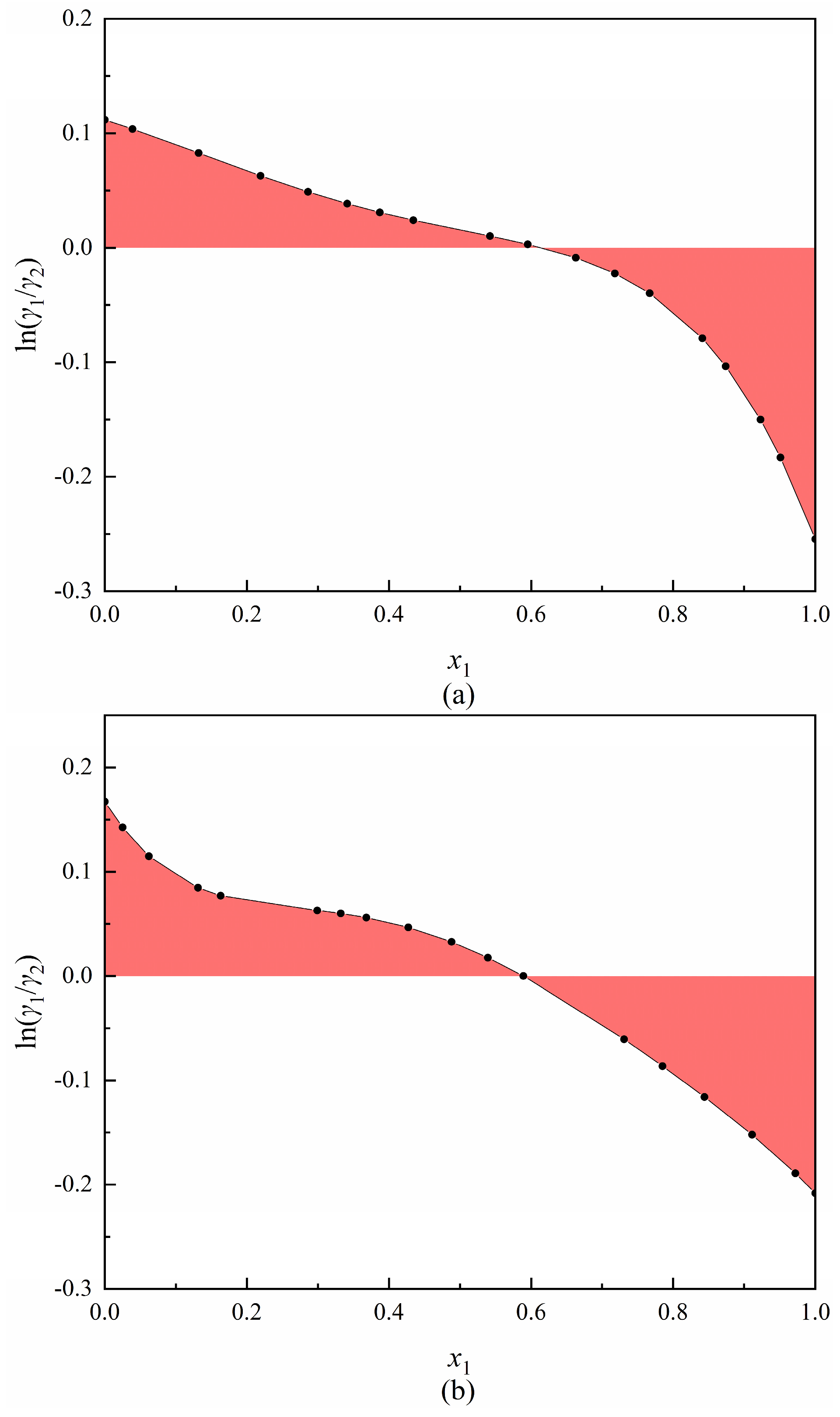
3.2. Thermodynamic Consistency Test

In this study, both the Redlich–Kister method [33] and the Van Ness method modified by Fredenslund [34] were used to check the thermodynamic consistency of VLE data.

The Redlich–Kister test is expressed as Equation (4).

$$D=100\frac{\left|{\displaystyle \int {}_0^1\ln ({\gamma }_1/{\gamma }_2)d{x}_1}\right|}{{\displaystyle \int {}_0^1\left|\ln ({\gamma }_1/{\gamma }_2)\right|d{x}_1}}\le 2$$

(4)

where γ₁ and γ₂ is the activity coefficient of component 1 and 2, respectively; x₁ is the mole fraction of component 1. When the value of D is no greater than 2 [33], the VLE data can be considered thermodynamically consistency. Meanwhile, the Redlich–Kister plots for two binary systems are illustrated in Figure 7.

The Van Ness method modified by Fredenslund, i.e., the Fredenslund test, is expressed as Equation (5).

$$\Delta y=\frac{1}{N}\underset{i=1}{\overset{N}{\Sigma }}\left|y_i^{\exp }-y_i^{cal}\right|\le 0.01$$

(5)

where N represents the number of experimental data points, y^exp is the experimental data of y, and y^cal is the calculated value. According to this method, the value of Δy should not be more than 0.01 for thermodynamic consistency [34].

Nevertheless, it should be noted that the Fredenslund test alone may not provide a comprehensive evaluation of thermodynamic consistency [35], as it does not consider potential local inconsistencies. Therefore, the residual disturbances of equilibrium temperature and vapor composition, as depicted in Figure 8 and Figure 9, should be analyzed. They were calculated from Equations (6) and (7) [36]. According to the distribution results in the figures, the data has local consistency.

$$\Delta T=T_{\exp }-T_{\mathrm{cal}}$$

(6)

$$\Delta y=y_{\exp }-y_{\mathrm{cal}}$$

(7)

The results of the Redlich–Kister test and the Fredenslund test are listed in

Table 3. The thermodynamic consistency test results.

System	D	Δy1 a
1,2-ED (1)—1,4-BD (2)	1.77	0.0014
1,3-PD (1)—1,4-BD (2)	0.22	0.0008

^a Testified by the NRTL model.

. The values of D for 1,2-ED (1) + 1,4-BD (2) and 1,3-PD (1) + 1,4-BD (2) are 0.9078 and 0.9321, respectively. They are both less than 2. Meanwhile, the Δy values are 0.0026 and 0.0018, respectively. They are both less than 0.01. Thus, the experimental VLE data for these two binary systems exhibit thermodynamic consistency.

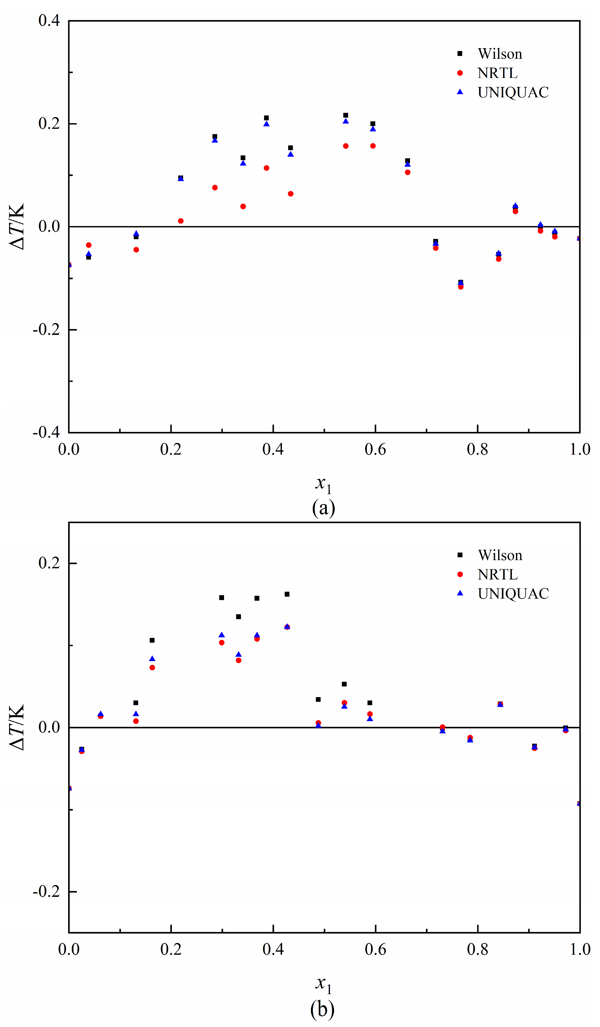
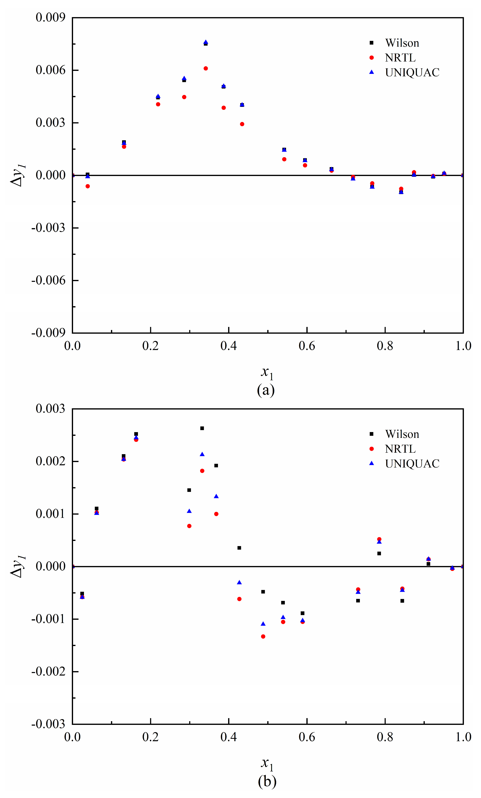
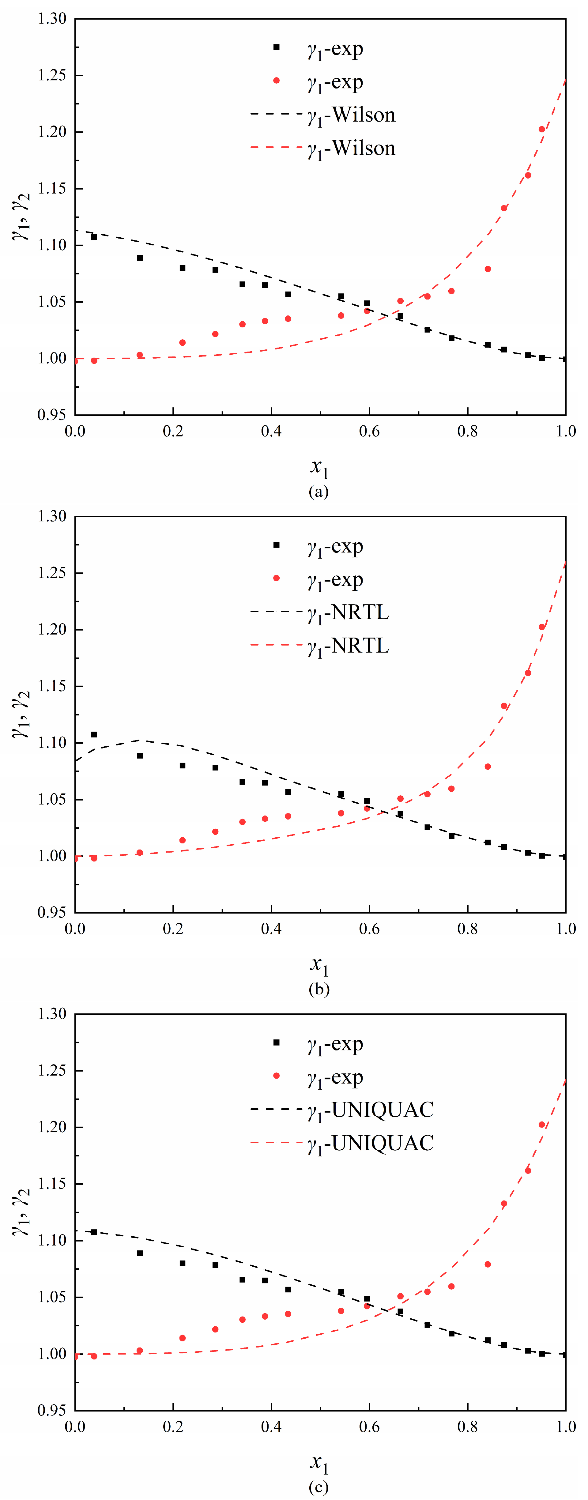
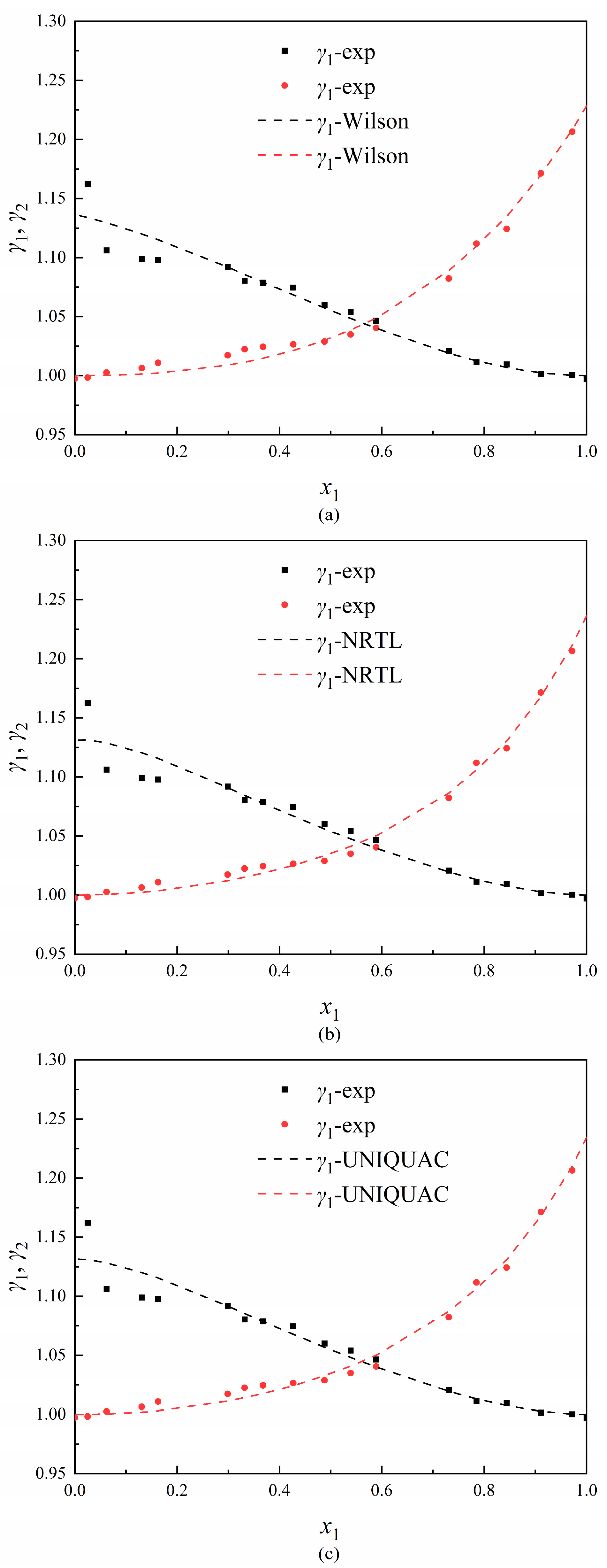
3.3. Data Regression

In this study, the Wilson, NRTL, and UNIQUAC activity coefficient models were used to regress the VLE data. These models can be found in Aspen Plus and listed in Appendix C. The maximum likelihood objective function was taken to regress the binary interaction parameters and expressed as Equation (8).

$$Q={\displaystyle \sum _{i=1}^N\left[{\left(\frac{p_i{}^{\exp }-p_i^{\mathrm{cal}}}{{\sigma }_p}\right)}^2+{\left(\frac{T_i^{\exp }-T_i^{\mathrm{cal}}}{{\sigma }_T}\right)}^2+{\left(\frac{x_{1,i}^{\exp }-x_{1,i}^{\mathrm{cal}}}{{\sigma }_x}\right)}^2+{\left(\frac{y_{1,i}^{\exp }-y_{1,i}^{\mathrm{cal}}}{{\sigma }_y}\right)}^2\right]}$$

(8)

where N is the number of experimental data, σ_T, σ_P, σ_x, and σ_y represent the standard deviations of T, p, x, and y, respectively. The nonrandom interaction parameter (α_ij) was set as 0.3 in the NRTL model.

Table 4. Correlated parameters of Wilson, NRTL, and UNIQUAC for 1,2-ED (1) + 1,4-BD (2) and 1,3-PD (1) + 1,4-BD (2).

Model	a12	a21	b12	b21	α
1,2-ED (1) + 1,4-BD (2)
Wilson	1.54	−5.40	−479.79	2111.72	-
NRTL	−19.57	12.58	9926.34	6373.18	0.3
UNIQUAC	−3.57	2.00	1497.94	−823.53	-
1,3-PD (1) + 1,4-BD (2)
Wilson	4.50	−8.26	−2057.22	3767.51	-
NRTL	−30.09	22.47	15,144.8	−11,261.3	0.3
UNIQUAC	11.57	−9.60	−5820.44	4809.73	-
1,2-ED (1) + 1,3-PD (2) α
Wilson	−141.12	91.50	0	0	-
NRTL	−14.78	50.33	0	0	0.3
UNIQUAC	116.52	−154.33	0	0	-

^α Binary interaction parameters used in simulation come from our previous work [17].

summarizes all the regressed binary interaction parameters.

Additionally, the root mean square deviation (RMSD) and average absolute deviation (AAD) were computed. When comparing experimental data with the calculated values, RMSD assesses how dispersed the data are, while ADD assesses how closely they coincide with each other.

As shown in

Table 5. AAD and RMSD for 1,2-ED (1) + 1,4-BD (2), and 1,3-PD (1) + 1,4-BD (2).

Model	AAD (T) a	AAD (y1) a	RMSD (T) b	RMSD (y1) b
1,2-ED (1) + 1,4-BD (2)
Wilson	0.10	0.0018	0.12	0.0029
NRTL	0.07	0.0014	0.08	0.0024
UNIQUAC	0.09	0.0018	0.11	0.0030
1,3-PD (1) + 1,4-BD (2)
Wilson	0.06	0.0009	0.08	0.0012
NRTL	0.05	0.0008	0.06	0.0011
UNIQUAC	0.05	0.0008	0.06	0.0011

^a AAD = $\frac{\sum _{i=1}^N\left|{\theta }_{i,exp}-{\theta }_{i,cal}\right|}{N}$, ^b RMSD = ${\left({\sum }_{i=1}^N\frac{{({\theta }_{i,exp}-{\theta }_{i,cal})}^2}{N}\right)}^{0.5}$. where N is the number of experimental data points, θ is the parameter (T and y in this study).

, the AAD of T is no more than 0.10 and 0.06, while the AAD of y₁ is no more than 0.0018 and 0.0009 for the two binary systems, respectively. RMSD of T is no more than 0.12 and 0.08, while RMSD of y₁ is no more than 0.0030 and 0.0012, respectively. Consequently, the VLE data can be effectively correlated using the three models. NRTL is taken for the following study because it presents the least AAD and RMSD for these two binary systems.

The T–x–y diagrams for experimental data and correlated data using the Wilson, NRTL, and UNIQUAC models for 1,2-EG (1) + 1,4-BD (2) and 1,3-PD (1) + 1,4-BD (2) are shown in Figure 10.

Meanwhile, the activity coefficient of experimental data and values calculated by the Wilson, NRTL, and UNIQUAC models for the two binary systems are shown in Figure 11 and Figure 12, respectively. These Figures show that the activity coefficient varies monotonically with liquid phase composition.

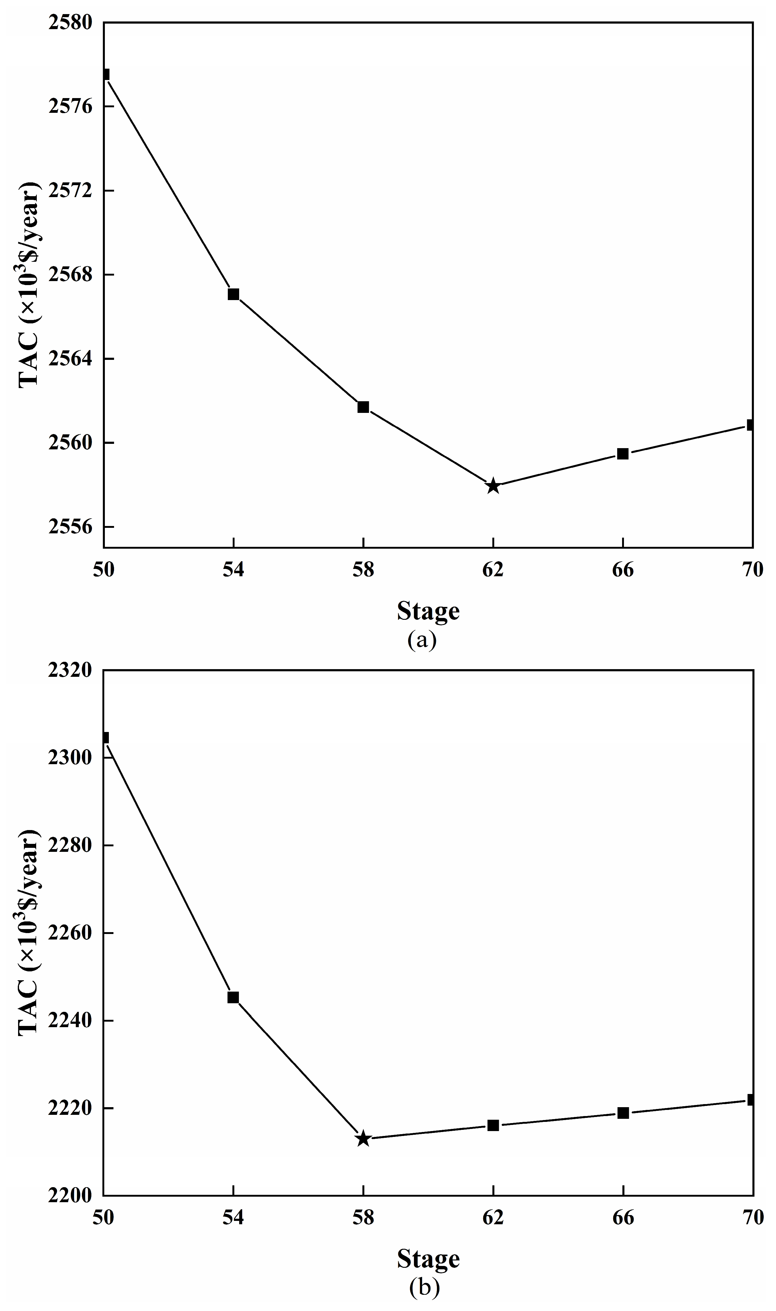
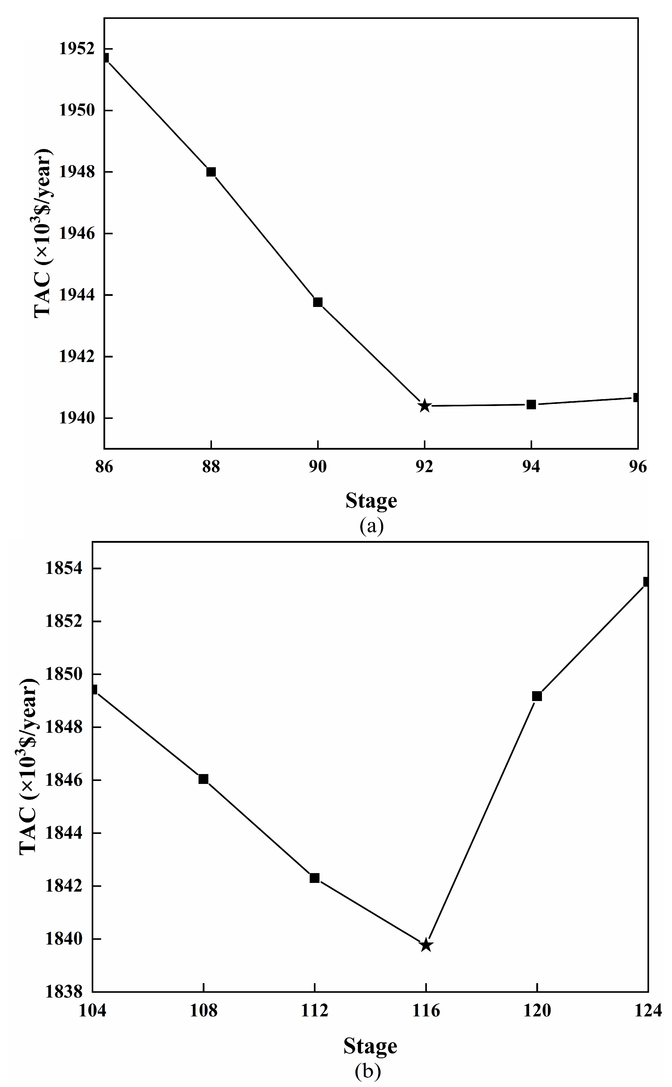
3.4. Optimization Results and Comparison

For DCDS, the optimization process can be found in Figure 13, which shows the relationship between TAC and the stages of C1 (NC1) and C2 (NC2). The TAC presents an initial rapid decrease with the increase of the two columns’ stages, followed by a gradual increase. The minimum TAC of 2,213,017 $/year for DCDS is achieved when N_C1 and N_C2 are 62 and 58, respectively. The optimization process for LDWC is illustrated in Figure 14, which displays the relationship between the stage in the left column CL (N_L) or right column CR (N_R) and TAC. The TAC first rapidly decreases, then slowly increases with the increasing N_L, while it rapidly decreases and then quickly increases with increasing N_R. The minimum TAC of 1,839,766 $/year for LDWC is obtained while the N_L is set as 92 and the N_R is 116.

The detailed costs for the optimized DCDS and LDWC are listed in

Table 6. Detailed cost of DCDS and LDWC.

	DCDS	LDWC
Capital cost ($)	2,028,300	2,178,246
Shell	1,196,753	1,409,168
Tray	89,091	128,568
Heat exchanger	742,456	640,510
CC Saving (%)	0	−7.39
Operating cost ($/year)	2,010,187	1,621,942
Heating utilities	1,936,378	1,586,162
Cooling utilities	73,809	35,779
OC Saving (%)	0	19.31
TAC * ($/year)	2,213,017	1,839,766
TAC Saving (%)	0	16.87

* The payback year was assumed at 10.

. Despite LDWC incurring a higher capital cost of 7.39% compared with DCDS, it involves a lower operating cost of 19.31% due to the lower energy requirement. As a result, TAC for LDWC can be reduced by 16.8% compared with DCDS.

The optimum design parameters for DCDS and LDWC are displayed in Figure 15, where 1,2-ED, 1,3-PD, and 1,4-BD are marked as A, B, and C, respectively. Figure 15a shows that the reboilers’ duties of DCDS are 4005 kW and 3234 kW, while the condensers’ duties of DCDS are 1697 kW and 3205 kW, respectively. From Figure 15b, the reboilers’ duties of LDWC are 3665 kW and 2181 kW, and the condensers’ duties of LDWC are 1356 kW and 2154 kW, respectively. As a result, LDWC achieves energy savings of 19.24% for heating utility and 28.40% for cooling utility than DCDS.

Figure 16 illustrates the liquid composition of C1 and C2 in DCDS. The concentrations of 1,2-ED and 1,4-ED exhibit a consistent monotonic change along the columns. However, the concentration of 1,3-PD within C1 presents two distinct peaks in the rectifying and stripping section, which requires additional energy to satisfy product specifications. As illustrated in Figure 17, 1,3-PD is withdrawn in the highest concentration zone for LDWC, which is similar to the DWC for ternary mixture separation and reduces the re-mixing of the middle component. Thus, LDWC has a lower energy consumption compared to DCDS.

4. Conclusions

In this study, we determine the VLE data for the binary systems of 1,2-ED + 1,4-BD and 1,3-PD + 1,4-BD at 101.3 kPa. Redlich–Kister and Fredenslund tests are employed to validate the reliability of measured data. The Redlich–Kister test parameter D is less than 2, and the Fredenslund test parameter Δy is less than 0.01, demonstrating that the VLE data present thermodynamic consistency. Additionally, VLE data are regressed using the Wilson, NRTL, and UNIQUAC activity coefficient models. AAD(T) and AAD(y₁) are no more than 0.10 K and 0.0018, respectively, and RMSD(T) and RMSD(y₁) are no more than 0.12 K and 0.0030, respectively, which indicate that the VLE data can be correlated well with all three models. Based on regression binary interaction parameters, DCDS and LDWC are designed and optimized for separating a ternary mixture including 1,2-ED, 1,3-PD, and 1,4-BD by the NRTL model. As a result, LDWC can reduce TAC by 16.87% and cooling and heating utility consumptions by 28.40% and 19.24%, respectively, compared with DCDS.

References

1. Liu, Y.; Wang, W.; Zeng, A.-P. Biosynthesizing structurally diverse diols via a general route combining oxidative and reductive formations of OH-groups. Nat. Commun. 2022, 13, 1595. [Google Scholar] [CrossRef] [PubMed]
2. Tronconi, E.; Ferlazzo, N.; Forzatti, P.; Pasquon, I.; Casale, B. A mathematical model for the catalytic hydrogenolysis of carbohydrates. Chem. Eng. Sci. 1992, 47, 2451–2456. [Google Scholar] [CrossRef]
3. Sholl, D.S.; Lively, R.P. Seven chemical separations to change the world. Nature 2016, 532, 435–437. [Google Scholar] [CrossRef] [PubMed]
4. Qian, X.; Liu, R.; Huang, K.; Chen, H.; Yuan, Y.; Zhang, L.; Wang, S. Comparison of Temperature Control and Temperature Difference Control for a Kaibel Dividing Wall Column. Processes 2019, 7, 773. [Google Scholar] [CrossRef]
5. Qian, X.; Liu, R.; Huang, K.; Chen, H.; Yuan, Y.; Zhang, L.; Wang, S. Controllability Comparison of the Four-Product Petlyuk Dividing Wall Distillation Column Using Temperature Control Schemes. Processes 2020, 8, 116. [Google Scholar] [CrossRef]
6. Rangaiah, G.P.; Feng, Z.; Hoadley, A.F. Multi-Objective Optimization Applications in Chemical Process Engineering: Tutorial and Review. Processes 2020, 8, 508. [Google Scholar] [CrossRef]
7. Ye, Q.; Wang, Y.; Pan, H.; Zhou, W.; Yuan, P. Design and Control of Extractive Dividing Wall Column for Separating Dipropyl Ether/1-Propyl Alcohol Mixture. Processes 2022, 10, 665. [Google Scholar] [CrossRef]
8. Kaibel, G. Distillation columns with vertical partitions. Chem. Eng. Technol. 1987, 10, 92–98. [Google Scholar] [CrossRef]
9. Dejanović, I.; Matijašević, L.; Halvorsen, I.J.; Skogestad, S.; Jansen, H.; Kaibel, B.; Olujić, Ž. Designing four-product dividing wall columns for separation of a multicomponent aromatics mixture. Chem. Eng. Res. Des. 2011, 89, 1155–1167. [Google Scholar] [CrossRef]
10. Kolbe, B.; Wenzel, S. Novel distillation concepts using one-shell columns. Chem. Eng. Process. Process Intensif. 2004, 43, 339–346. [Google Scholar] [CrossRef]
11. Ling, H.; Luyben, W.L. Temperature Control of the BTX Divided-Wall Column. Ind. Eng. Chem. Res. 2010, 49, 189–203. [Google Scholar] [CrossRef]
12. Si, Z.; Chen, H.; Cong, H.; Li, X. Energy, exergy, economic and environmental analysis of a novel steam-driven vapor recompression and organic Rankine cycle intensified dividing wall column. Sep. Purif. Technol. 2022, 295, 121285. [Google Scholar] [CrossRef]
13. Ramapriya, G.M.; Tawarmalani, M.; Agrawal, R. Thermal coupling links to liquid-only transfer streams: A path for new dividing wall columns. AIChE J. 2014, 60, 2949–2961. [Google Scholar] [CrossRef]
14. Cui, C.; Zhang, X.; Sun, J. Design and optimization of energy-efficient liquid-only side-stream distillation configurations using a stochastic algorithm. Chem. Eng. Res. Des. 2019, 145, 48–52. [Google Scholar] [CrossRef]
15. Cui, C.; Zhang, Q.; Zhang, X.; Sun, J. Eliminating the vapor split in dividing wall columns through controllable double liquid-only side-stream distillation configuration. Sep. Purif. Technol. 2020, 242, 116837. [Google Scholar] [CrossRef]
16. Zhang, T.; Li, M.; Pan, H.; Ling, H. Dynamic control of liquid-only transfer Kaibel dividing-wall column. Chem. Eng. Sci. 2023, 272, 118589. [Google Scholar] [CrossRef]
17. Qu, X.C.; Wu, Y.Y.; Zhu, J.W.; Chen, K.; Wu, B.; Ji, L.J. Separation of ternary system (1,2-ethanediol+1,3-butanediol+1,3-propanediol) by distillation. Sep. Sci. Technol. 2018, 53, 2435–2443. [Google Scholar] [CrossRef]
18. Yang, C.; Sun, Y.; Qin, Z.; Feng, Y.; Zhang, P.; Feng, X. Isobaric Vapor–Liquid Equilibrium for Four Binary Systems of Ethane-1,2-diol, Butane-1,4-diol, 2-(2-Hydroxyethoxy)ethan-1-ol, and 2-[2-(2-Hydroxyethoxy)ethoxy]ethanol at 10.0 kPa, 20.0 kPa, and 40.0 kPa. J. Chem. Eng. Data 2014, 59, 1273–1280. [Google Scholar] [CrossRef]
19. Wilson, G.M. Vapor-liquid equilibrium. XI. A new expression for the excess free energy of mixing. J. Am. Chem. Soc. 1964, 86, 127–130. [Google Scholar] [CrossRef]
20. Renon, H.; Prausnitz, J.M. Local compositions in thermodynamic excess functions for liquid mixtures. AIChE J. 1968, 14, 135–144. [Google Scholar] [CrossRef]
21. Abrams, D.S.; Prausnitz, J.M. Statistical thermodynamics of liquid mixtures: A new expression for the excess Gibbs energy of partly or completely miscible systems. AIChE J. 1975, 21, 116–128. [Google Scholar] [CrossRef]
22. Rodrigues, M.; Francesconi, A.Z. Experimental Study of the Excess Molar Volumes of Binary and Ternary Mixtures Containing Water +(1,2-Ethanediol, or 1,2-Propanediol, or 1,3-Propanediol, or 1,2-Butanediol) + (1-n-Butyl-3-methylimidazolium Bromide) at 298.15 K and Atmospheric Pressure. J. Solut. Chem. 2011, 40, 1863–1873. [Google Scholar] [CrossRef]
23. Zhang, K.; Meng, X.Y.; Wu, J.T. Flammability Limits of Binary Mixtures of 1,2-Ethanediol plus Steam and 1,2-Propanediol plus Steam. J. Chem. Eng. Data 2013, 58, 2681–2686. [Google Scholar] [CrossRef]
24. Lin, Y.F.; Tu, C.H. Isobaric vapor-liquid equilibria for the binary and ternary mixtures of 2-propanol, water, and 1,3-propanediol at P = 101.3 kPa: Effect of the 1,3-propanediol addition. Fluid Phase Equilib. 2014, 368, 104–111. [Google Scholar] [CrossRef]
25. Zhong, Y.; Wu, Y.Y.; Zhu, J.W.; Chen, K.; Wu, B.; Ji, L.J.; Shen, Y.L. The Distillation Process Design for the Ternary System 1,2-Butanediol + 1,4-Butanediol + 2,3-Butanediol. Sep. Sci. Technol. 2015, 50, 2545–2552. [Google Scholar] [CrossRef]
26. Zhai, X.; Wu, Y.; Tian, B.; Yao, Y.; Wu, B.; Chen, K.; Ji, L. Isobaric Vapor-Liquid Equilibrium for the Binary System of Cumene plus Acetophenone at 101.3, 30.0, and 10.0 kPa. J. Chem. Eng. Data 2022, 67, 669–675. [Google Scholar] [CrossRef]
27. Yi, Q.; Chen, W.P.; Zhang, X.Y.; Wu, Y.Y.; Wu, B.; Chen, K.; Ji, L.J. Isobaric Vapor–Liquid Equilibrium for the Binary Systems of 2-Phenylethanol + 2-Ethylphenol, 1-Phenyl-2-propanol + 2-Ethylphenol, 2-Phenylethanol + 1-Phenyl-2-propanol and 2-Phenyl-1-propanol + 2-Ethylphenol under 101.3 kPa. J. Chem. Eng. Data 2021, 66, 4351–4360. [Google Scholar] [CrossRef]
28. Chen, M.; Yu, N.; Cong, L.; Wang, J.; Zhu, M.; Sun, L. Design and Control of a Heat Pump-Assisted Azeotropic Dividing Wall Column for EDA/Water Separation. Ind. Eng. Chem. Res. 2017, 56, 9770–9777. [Google Scholar] [CrossRef]
29. Lee, H.-Y.; Yeh, M.-H.; Chen, Y.-Y.; Chen, C.-L. Design and control of a comprehensive Ethylenediamine (EDA) process with external/internal heat integration. Sep. Purif. Technol. 2022, 293, 121137. [Google Scholar] [CrossRef]
30. Liu, Y.; Zhai, J.; Li, L.; Sun, L.; Zhai, C. Heat pump assisted reactive and azeotropic distillations in dividing wall columns. Chem. Eng. Process. Process Intensif. 2015, 95, 289–301. [Google Scholar] [CrossRef]
31. Douglas, J.M. Conceptual Design of Chemical Processes; McGraw-Hill: New York, NY, USA, 1988. [Google Scholar]
32. Zheng, H.; Luo, X.; Yin, G.; Chen, J.; Zhao, S. Vapor Pressure and Isobaric Vapor–Liquid Equilibrium for Binary Systems of Furfural, 2-Acetylfuran, and 5-Methylfurfural at 3.60 and 5.18 kPa. J. Chem. Eng. Data 2018, 63, 49–56. [Google Scholar] [CrossRef]
33. Redlich, O.; Kister, A.T. Thermodynamics of Nonelectrolyte Solutions-x-y-t relations in a Binary System. Ind. Eng. Chem. Res. 1948, 40, 341–345. [Google Scholar] [CrossRef]
34. Fredenslund, A.; Gmehling, J.; Rasmussen, P. Vapor–Liquid Equilibria Using UNIFAC—A Group Contribution Model; Elsevier: Amsterdam, The Netehrlands, 1977. [Google Scholar]
35. Mathias, P.M. Effect of VLE uncertainties on the design of separation sequences by distillation—Study of the benzene–chloroform–acetone system. Fluid Phase Equilib. 2016, 408, 265–272. [Google Scholar] [CrossRef]
36. Sosa, A.; Ortega, J.; Fernández, L.; Pacheco, J.M.; Wisniak, J.; Romero, A. Further Advance to a Practical Methodology to Assess Vapor–Liquid Equilibrium Data: Influence on Binaries Rectification. J. Chem. Eng. Data 2019, 64, 3933–3944. [Google Scholar] [CrossRef]
37. Kiss, A.A. Advanced Distillation Technologies: Design, Control, and Applications; Wiley: Chichester, UK, 2013. [Google Scholar]
38. Cui, C.; Li, X.; Guo, D.; Sun, J. Towards energy efficient styrene distillation scheme: From grassroots design to retrofit. Energy 2017, 134, 193–205. [Google Scholar] [CrossRef]
39. Luyben, W.L. Distillation Design and Control Using Aspen™ Simulation; John Wiley & Sons, Inc.: Hoboken, NY, USA, 2013. [Google Scholar]
40. Song, Z.-W.; Cui, W.; Wu, Y.-Y.; Wu, B.; Chen, K.; Ji, L.-J. Energy, exergy, economic, and environmental analysis of a novel liquid-only transfer dividing wall column with vapor recompression. Sep. Purif. Technol. 2024, 329, 125122. [Google Scholar] [CrossRef]
41. Li, Q.; Feng, Z.; Rangaiah, G.P.; Dong, L. Process Optimization of Heat-Integrated Extractive Dividing-Wall Columns for Energy-Saving Separation of CO2 and Hydrocarbons. Ind. Eng. Chem. Res. 2020, 59, 11000–11011. [Google Scholar] [CrossRef]
42. Sun, L.-Y.; Chang, X.-W.; Qi, C.-X.; Li, Q.-S. Implementation of Ethanol Dehydration Using Dividing-Wall Heterogeneous Azeotropic Distillation Column. Sep. Sci. Technol. 2011, 46, 1365–1375. [Google Scholar] [CrossRef]
43. Sun, L.; Wang, Q.; Li, L.; Zhai, J.; Liu, Y. Design and Control of Extractive Dividing Wall Column for Separating Benzene/Cyclohexane Mixtures. Ind. Eng. Chem. Res. 2014, 53, 8120–8131. [Google Scholar] [CrossRef]
Figure 1. Diagrammatic schematic of LDWC. Where DFCL is the distillate flow rate of CL, DFCR is the distillate flow rate of CR, and FB is the flow rate of B.
Processes 11 03150 g001
Figure 2. Diagrammatic schematic of DCDS. Where DFC1 is the distillate flow rate of C1, DFC2 is the distillate flow rate of C2.
Processes 11 03150 g002
Figure 3. Apparatus for the VLE: (1) electric heating rod; (2) a port for liquid-phase sampling; (3) thermometer; (4) condenser tube; (5) U-shaped mercury differential manometer; (6) a port for vapor-phase sampling; (7) nitrogen cylinder; and (8) buffer vessel.
Processes 11 03150 g003
Figure 4. The equivalent model for LDWC in Aspen Plus.
Processes 11 03150 g004
Figure 5. Optimization procedure for DCDS.
Processes 11 03150 g005
Figure 6. Optimization procedure for LDWC.
Processes 11 03150 g006
Figure 7. Redlich–Kister plots for the binary system of (a) 1,2-ED (1) + 1,4-BD (2), (b) 1,3-PD (1) + 1,4-BD (2).
Processes 11 03150 g007
Figure 8. Residual disturbance for the equilibrium temperature (T) with liquid composition (x1) of (a) 1,2-ED (1) + 1,4-BD (2), (b) 1,3-PD (1) + 1,4-BD (2).
Processes 11 03150 g008
Figure 9. Residual disturbance for vapor composition (y1) with liquid composition (x1) of (a) 1,2-ED (1) + 1,4-BD (2), (b) 1,3-PD (1) + 1,4-BD (2).
Processes 11 03150 g009
Figure 10. T–x–y diagram for (a) 1,2-EG (1) + 1,4-BD (2) and (b) 1,3-PD (1) + 1,4-BD (2) at 101.3 kPa using Wilson, NRTL, and UNIQUAC models.
Processes 11 03150 g010
Figure 11. The activity coefficient for experimental and correlated data for 1,2-EG (1) + 1,4-BD (2) using (a) Wilson, (b) NRTL, and (c) UNIQUAC models.
Processes 11 03150 g011
Figure 12. The activity coefficient for experimental and correlated data for 1,3-PD (1) + 1,4-BD (2) using (a) Wilson, (b) NRTL, and (c) UNIQUAC models.
Processes 11 03150 g012
Figure 13. The relationship between TAC and stages of (a) C1 and (b) C2 for DCDS.
Processes 11 03150 g013
Figure 14. The relationship between TAC and stages of (a) CL and (b) CR for LDWC.
Processes 11 03150 g014
Figure 15. Simulation results of (a) DCDS and (b) LDWC.
Processes 11 03150 g015
Figure 16. Liquid composition profiles of (a) C1, (b) C2 in DCDS.
Processes 11 03150 g016
Figure 17. Liquid profiles of (a) CL and (b) CR in LDWC.
Processes 11 03150 g017