A Novel Convolutional LSTM Network Based on the Enhanced Feature Extraction for the Transmission Line Fault Diagnosis

Abstract

Recently, the traditional transmission line fault diagnosis approaches cannot handle the variables’ dynamic coupling properties, and they also ignore the local structure feature information during the feature extraction. To figure out these issues, a novel enhanced feature extraction based convolutional LSTM (ECLSTM) approach is developed to diagnose the transmission line fault in this paper. Our work has three main contributions: (1) To tackle the dynamic coupling characteristics of the process variables, the statistics analysis (SA) method is first employed to calculate different statistical features of the transmission line’s original data, where the original datasets are transformed into the subsequently used statistics datasets; (2) The statistics comprehensive feature preserving (SCFP) is then proposed to maintain both the global and local structure features of the constructed statistics datasets, where the locality structure preserving technique is incorporated into the principal component analysis (PCA) model to extract the features from the statistics datasets; (3) To effectively diagnose the transmission line’s fault, the SCFP based convolutional LSTM fault diagnosis scheme is constructed to classify the global and local statistical structure features of fault snapshot dataset, because of its ability to exploit the temporal dependencies and spatial correlations of the extracted statistical features. Detailed experiments and comparisons on the datasets of the simulated power system are performed to prove the excellent performance of the ECLSTM based fault diagnosis scheme.

1. Introduction

1.1. Motivation and Incitement

As an important component of the power system, the transmission line transmits the power from the source area to the distribution network [1]. However, the transmission line’s fault always affects the power supply and reliability of the power system [2]. Under this background, efficient fault diagnosis schemes for the transmission line are urgently needed to remove these faults and guarantee the power system is running safely [3]. For many data-driven transmission line recognition models, the original datasets are often used as the input. Thus, these models cannot cope with the dynamic coupling properties between different original variables [4]. However, the effectiveness of fault diagnosis approaches for the transmission line is seriously affected by the original variables’ dynamically correlated natures [5].

To deal with the dynamic coupling characteristics contained in the original process variables, some fault diagnosis methods based on mining the higher-order statistics of the original process variables have been studied in recent years. For example, as an emerging superior feature extraction technique, statistics analysis (SA) [6,7] has been developed to calculate multiple different statistical indicators among different process variables for the purpose of tackling coupling dynamics. The original variables’ interaction and relevance can be sufficiently revealed and captured by calculating and grouping the multiple statistics of the original process variables. Hence, in our work, the SA method is utilized to figure out the dynamic interactions between the original variables of the transmission line.

Although the dynamic correlative properties among the original measured variables can be successfully figured out by the SA, the redundant information between the calculated multiple statistics always leads to an adverse impact on the fault diagnosis of the transmission line. In view of the PCAs superiority in removing redundant information among the multiple statistics by preserving the main variance information, we intend to apply the PCA to characterize the transmission line’s running state by retaining the key latent statistics. However, the traditional PCA-based approach only mines the global structure features and neglects the important local structure features [8]. Recently, locality-preserving-based methods have been suggested to exploit the local neighbor structure of the samples for feature extraction by considering the underlying geometrical manifold of the dataset [9,10]. In our work, a novel dimension reduction technique, i.e., comprehensive feature preservation (CFP), is proposed to mine the global and local data structures of the different statistics by combining the advantages of the PCA and locality preservation techniques together.

According to the above analysis, if the statistics analysis (SA) method is integrated into the constructed CFP technique, the improved feature extraction model will capture the dynamic interactions among the original variables as well as remove redundant correlation information by preserving the data’s global and local structure. As a result, the transmission line’s fault diagnosis performance will be significantly improved by employing the constructed feature extraction model to exploit the data features during the dimensionality reduction. Inspired by the merits of the SA method and the CFP technique, we have come up with an enhanced feature extraction strategy termed the statistics CFP (SCFP) by combining the SA with the CFP in our work.

After the global and local statistical features of the fault snapshot dataset are extracted, it is also very important to recognize the fault patterns of the transmission line. Although long short-term memory (LSTM) [11,12] has been widely applied to recognize the fault type in the fault diagnosis field, conventional LSTM only focuses on the data’s temporal dependency information and ignores the spatial structure information. As an improved version of the LSTM, the convolutional LSTM (CLSTM) owns the superiority to keep the data’s temporal dependencies, such as the LSTM, and consider the data’s spatial correlation, such as the CNN, which has been widely applied to perform the classification tasks recently [13]. Because of the CLSTMs above merits in identifying the fault pattern, in this paper, we adopt the CLSTM-based approach to recognize the reinforced data features mined by the suggested SCFP model.

1.2. Literature Review

Modern power systems exhibit very rapid development in the complexity of power transmission and supply to satisfy the increasing energy requirement [1]. However, faults frequently occur in the transmission line, which impacts the power supply and degrades the reliability of the power system [14]. Therefore, to maintain the damaged components and reduce the downtime, it is crucial to accurately diagnose the transmission line faults and rapidly eliminate the faults.

With the progress of data measurement and collection systems, massive transmission line-running data becomes available. Based on the gathered running data, data-driven approaches are gaining more and more attention to diagnose transmission line faults [15,16]. However, the most data-driven models cannot cope with the coupling dynamics of the process data because their input datasets are directly collected from the original process variables. In practice, the dynamic properties would lead the process variables to be interrelated and influenced, which always influences the fault identification accuracy of the abovementioned methods.

Recently, by mining the higher-order statistics of original process variables, some fault diagnosis methods have been discussed to handle the variables’ dynamic coupling characteristics. For instance, the independent component analysis (ICA)-based fault diagnosis approaches adopt higher-order statistical information to discover the independent and non-Gaussian distributed latent features from the original measured variables, which can reveal more useful fault information [17,18]. However, the ICA-based methods have the limitation of dealing with the measurement noise hidden in the collected data. When the gathered data are contaminated with measurement noise, the latent variables cannot be precisely derived [19]. As an alternative way to tackle the coupling dynamics, statistics analysis (SA) [6,7] has been reported to calculate the variables’ multiple different statistical indicators. Another merit of the statistics analysis (SA) is that regardless of the original variables’ non-Gaussian distribution, the computed statistics of the variables will follow the Gaussian distribution [5]. Hence, the calculated statistical features are efficient in clearing off the bad effect of the original variables’ interactional dynamics on the fault recognition performance.

To further remove the redundant information between the calculated multiple statistics, the principal component analysis (PCA) has been applied to extract the intrinsic latent variables by preserving the main variance information recently [20,21]. In this way, the PCA can capture the global structure of the process data for feature extraction. However, the traditional PCA-based approach only mines the global structure features and neglects the important local structure features for eliminating redundant features among the computed statistics [8]. The local structure features are also significant for feature extraction because they indicate the detailed neighbor relations of different samples [22]. The loss of this crucial information in low-dimensional space may have a great impact on dimension reduction performance.

As mentioned above, the local structure features are also significant for feature extraction and dimensionality reduction because they indicate the detailed neighbor relations of different samples [22]. The missed local structure would result in the downside influence of eliminating the redundant information and extracting the key latent features. Recently, locality-preserving-based methods have been suggested to exploit the local neighbor structure of the samples for feature extraction by considering the underlying geometrical manifold of the dataset [9,10]. However, without preserving the variance information, the outer shape of the dataset may be broken after the dimension reduction procedure. Hence, the performance of local feature extraction may be degraded if a dataset has significant directions for variance information.

After the global and local statistical features of the process data are extracted, the next work is to effectively analyze these mined fault features for the transmission line’s fault pattern recognition. In recent years, deep neural network-based methods have displayed superior capability to exploit the valuable information from the process data [23,24]. As a classical deep learning method, long short-term memory (LSTM) [11,12] is widely applied to recognize fault types in the fault diagnosis field. For instance, Sun et al. [25] combined the LSTM model with Bayesian to perform the fault diagnosis task for the nonlinear dynamic process. To monitor the milling process under different working conditions, Zheng et al. discussed an attention mechanism-combined LSTM to estimate the tool wear value [26]. Zhou et al. combined the entropy-based sparsity measure with the LSTM to carry out the bearing defect prognosis [27]. To carry out the fault classification and fault prediction of the transmission line, Belagoune et al. [14] employed the LSTM-based approach to classify and predict the multivariate temporal sequences. To acquire improved fault identification results, Han et al. [28] discussed a modified memory-capable-based LSTM approach to select the optimal hidden layer node number. However, the traditional LSTM merely utilizes the previous samples’ useful information to derive the output at present. Thus, the conventional LSTM only focuses on the data’s temporal dependency information and ignores the spatial structure information.

As an improved version of the LSTM, the convolutional LSTM (CLSTM) has been proposed by displacing matrix multiplication in the traditional LSTM with a convolution operation. The CLSTM has the superiority to keep the data’s temporal dependencies, such as the LSTM, and consider the data’s spatial correlation, such as the CNN, which has been widely applied to perform the classification tasks recently [26]. For example, Nogas et al. [29] proposed CLSTM-based spatiotemporal autoencoders to implement the fall detection task. To deal with the problem of deepfake video detection, Chen et al. [30] suggested the Xception-LSTM algorithm to capture and enhance the frame spatial structure features and temporal dependencies by combining the spatiotemporal attention mechanism with the CLSTM. Based on a modified CLSTM, Yu et al. [31] proposed an improved autoencoder network to effectively extract the key features of the measured data for fault detection in industrial processes. Considering the CLSTMs merits, we adopt the CLSTM-based approach to recognize the reinforced data features mined by the suggested SCFP model.

1.3. Contributions and Paper Organization

To exploit much more comprehensive and detailed feature information from the transmission line fault data, an effective combination of the SA method and the CFP technique is proposed to mine the data features in our work. Furthermore, if the CLSTM model is utilized to identify the enhanced data features, much better fault diagnosis performance of the transmission line will be achieved. In short, this paper proposes an enhanced feature extraction-based CLSTM method to identify the transmission line’s faults. The main innovations and contributions are given out.

(1) To cope with the dynamic coupling properties hidden in the process variables, the SA method is applied to calculate different statistical features of the transmission line’s original data. In the SA, the behaviors of the transmission line are characterized by computing the statistics pattern, which contains different order statistics with the help of the moving window technique. The training statistics matrix is then built by gathering the multiple computed statistics patterns from different moving windows, which is efficient to clear off the bad effect of the original variables’ interactional dynamics on the subsequent fault diagnosis.

(2) To further eliminate the redundant correlation information among the calculated multiple statistics, a novel SCFP model is developed to carry out the feature extraction. The SCFP model has the capability to mine the global and local structure features of the constructed training statistics matrix during dimension reduction. Specifically, considering the traditional PCA only maintains the global structure feature for dimensionality reduction, the locality structure preservation is combined into the PCA to establish the SCFP model.

(3) To effectively diagnose the fault of the transmission line, the SCFP-based ECLSTM fault identification is suggested to exploit the temporal dependencies and spatial correlations of the mined global and local statistical features. Firstly, the fault samples are collected to set up the snapshot dataset. Then, the SCFP model is employed to extract the global and local statistical features of the current snapshot dataset. And, to train the fault diagnosis model, the mined global and local statistical features of multiple historical fault datasets are input to the CLSTM. At last, the ECLSTM diagnosis model is applied to classify the snapshot dataset’s global and local statistical features to diagnose the fault.

(4) To fully verify the performance of the proposed ECLSTM-based transmission line diagnosis scheme, the ECLSTM model is compared with some closely related diagnosis models in terms of diagnosing the fault. The experiments of the suggested ECLSTM and the comparisons with related approaches are carried out on the datasets of the simulated power system. In comparison with the related methods, the fault diagnosis results display the superior effectiveness of the ECLSTM-based recognition scheme.

The other parts of this paper are given out. Section 2 introduces the transmission line’s short circuit faults, the basic PCA, and the convolutional LSTM. The SCFP-based feature extraction technique is developed in Section 3. The ECLSTM-based transmission line fault diagnosis approach is established in Section 4. The case study on the datasets of the simulated power system is implemented in Section 5. At last, the conclusion is formulated in Section 6.

2. Preliminaries

2.1. The Short Circuit Faults of the Transmission Line

The transmission line usually experiences short circuit faults, which always lead to residual life reduction, power loss increase, and so on [32]. Different short circuit faults always arise during the transmission line’s daily running, which can be divided into asymmetrical faults and symmetrical faults [14]. To be specific, the line-to-ground (LG) faults, the line-to-line (LL) faults, and the double lines-to-ground (LLG) faults belong to the asymmetrical faults, which possess a much higher occurrence probability compared with the symmetrical faults [33]. On the other hand, the triple lines (LLL) faults and the triple lines to ground (LLLG) faults remain with the symmetrical faults, which result in much greater damage to the transmission line than the asymmetrical faults [33]. However, the occurrence probability of these symmetrical faults is smaller than that of the asymmetrical faults.

The short circuit faults seriously influence the running status of the transmission line; therefore, the rapid and accurate recognition of the short circuit faults is significant and important to ensuring the safe and stable operation of the transmission line [34,35]. According to the specific fault pattern, the amplitude, phase, and frequency of the voltages and currents for the short circuit faults would undergo obvious changes, and these changes are unique to each fault pattern. In this way, we can capture the covariate features from the short circuit faults’ temporal operation data to discern different fault patterns as well as process disturbances.

2.2. The Basic PCA Method

The PCA possesses the ability to cope with highly redundant process data by mapping the redundant data into a low-dimensional principal component subspace that contains the most variations of the data [8,20,21]. Therefore, the PCA is widely used for data feature extraction.

Suppose this $X\in R^{n\times m}$ is the original high-dimensional dataset, which contains n samples, and each sample consists of m measured variables. After the dataset X is scaled according to the normal operation dataset, the covariance S of the dataset X is first computed

$$S=\frac{1}{n-1}{X}^{\mathrm{T}}X$$

(1)

Then, Equation (2) is carried out on the obtained covariance, which is given out as follows:

$$S=VD{V}^{\mathrm{T}}$$

(2)

where D represents a diagonal matrix, whose diagonal contains the decreasing-order eigenvalues ${\tilde{\lambda }}_1>{\tilde{\lambda }}_2>\dots >{\tilde{\lambda }}_{rank(X)}$ of the matrix S. The l eigenvectors ${\tilde{p}}_1,{\tilde{p}}_2,\dots ,{\tilde{p}}_l$ of the matrix S corresponding to the first l largest eigenvalues ${\tilde{\lambda }}_1>{\tilde{\lambda }}_2>\dots >{\tilde{\lambda }}_l$ are retained to construct the loading matrix $\tilde{P}=[{\tilde{p}}_1,{\tilde{p}}_2,\dots ,{\tilde{p}}_l]\in R^{m\times l}$.

Based on the loading matrix $\tilde{P}$, the original dataset X is mapped into the principal component and residual spaces.

$$X=T{\tilde{P}}^{\mathrm{T}}+E=t_1{\widetilde{p_1}}^{\mathrm{T}}+t_2{\widetilde{p_1}}^{\mathrm{T}}+\cdots +t_l{\widetilde{p_l}}^{\mathrm{T}}+E$$

(3)

where T indicates the score matrix $T=[t_1,t_2,\cdots ,t_l]$, and $t_i\in R^n$ is the i-th score vector. Note that, the vector ${\tilde{p}}_i$ is also called the i-th loading vector, and the l also represents the principal component (PC) number retained in the principal space.

The residual matrix E in residual space is computed as

$$E=X-\widehat{X}=X-T{\tilde{P}}^{\mathrm{T}}$$

(4)

In the principle component space, the computed PCs can represent the main changes of the process. While the latent variables in the residual space characterize the process noise information.

2.3. The Basic Convolutional LSTM Network

The traditional LSTM network only maintains the data’s temporal dependencies and omits the data’s spatial correlations. By incorporating the convolution operation into the LSTM, Shi et al. [36] proposed the convolutional LSTM (CLSTM) to handle both the temporal dependencies and the spatial correlations of video data.

The CLSTM adopts a convolutional structure to replace the fully connected layer in the traditional LSTM; therefore, the CLSTM not only owns the LSTMs advantage to mine the temporal relations of process data but also inherits the CNNs merit to exploit the local spatial features. Figure 1 gives out the schematic diagram of the CLSTM. The input of the CLSTM has three portions: the previous memory information, the previous unit’s output, and the current input. As displayed in Figure 1, the CLSTM consists of an input gate, an output gate, a forget gate, and a memory unit, which makes the CLSTM take advantage of the spatiotemporal features of the process data effectively.

The forget gate abandons unnecessary information selectively, which is formulated as

$$f_t=\sigma (W_f\odot [c_{t-1},h_{t-1},x_t]+b_f)$$

(5)

where $\sigma$ indicates activation function, $\odot$ is convolution operation, $x_t$ indicates input vector at sample interval t, $c_{t-1}$ indicates previous information, $h_{t-1}$ represents previous output of the CLSTM unit, and $W_f$ and $b_f$ are respectively the weight and bias of the forget gate.

In general, to selectively pass the information through, the activation function $\sigma$ is always chosen as the sigmoid function to convert the input x_i into the range (0, 1).

$$\sigma (x_i)=\mathrm{sigmoid}(x_i)=\frac{1}{1+e^{-x_i}}$$

(6)

The input gate adds new information to the memory unit, where the information is first determined for updating, and then the alternative information is generated.

$$i_t=\sigma (W_i\odot [c_{t-1},h_{t-1},x_t]+b_i)$$

(7)

$${\tilde{C}}_t=\tan \mathrm{h}(W_c\odot [h_{t-1},x_t]+b_c)$$

(8)

where $i_t$ and ${\tilde{C}}_t$ are respectively the input gate’s output and the memory unit’s alternative information, and tanh represents the tangent function.

The memory information $C_t$ is updated as follows:

$$C_t=f_t·C_{t-1}+i_t·{\tilde{C}}_t=f_t·C_{t-1}+i_t·\tan \mathrm{h}(W_c\odot [h_{t-1},x_t]+b_c)$$

(9)

where the C_t integrates the previous $C_{t-1}$ and current states ${\tilde{C}}_t$ to construct the CLSTMs memory state.

Based on the above computation, the output gate provides the final output.

$$o_t=\sigma (W_o\odot [c_t,h_{t-1},x_t]+b_o)$$

(10)

$$h_t=o_t·\tanh (C_t)$$

(11)

where $o_t$ is the output gate’s output, and $h_t$ is the output of the CLSTM at sample interval t.

3. The Developed SCFP Based Feature Extraction Technique

3.1. The SA Method

To figure out the transmission line’s dynamic interactions among original process variables, the statistics analysis (SA) approach is first employed to exploit the original variables’ statistical features in the developed SCFP technique. To be specific, in the SA method, the process operation state is characterized by variables’ different statistics.

For the normal operating dataset X, let the subset $X_k$ indicate a window of samples, which is formulated as

$$X_k=\left[\begin{array}{cccc}{x}_1(k-w+1)& x_2(k-w+1)& \cdots & x_m(k-w+1)\\ x_1(k-w+2)& x_2(k-w+2)& \cdots & x_m(k-w+2)\\ ⋮& ⋮& \ddots & ⋮\\ x_1(k)& x_2(k)& \cdots & x_m(k)\end{array}\right]$$

(12)

where $w$ represents the window width and $k$ indicates the current time index. The SA is indeed to calculate the statistics pattern (SP), which contains four statistics: mean, variance, skewness, and kurtosis. To be specific, the mean of the original process variables is calculated as

$$u_i=\frac{1}{w}{\displaystyle \sum _{l=0}^{w-1}{x}_i(k-l)}, i=1,2,\cdots ,m$$

(13)

The second-order statistic is the variance of the original process variables, which is formulated as

$$v_i=\frac{1}{w}{\displaystyle \sum _{l=0}^{w-1}{[x_i(k-l)-u_i]}^2}, i=1,2,\cdots ,m$$

(14)

The skewness measures the nonlinearity of original variables, and the kurtosis evaluates the non-Gaussianity of original variables. Specifically, the skewness and kurtosis are respectively expressed as

$${\gamma }_i=\frac{\frac{1}{w}{\displaystyle \sum _{l=0}^{w-1}[x_i}(k-l)-u_i{]}^3}{{\left(\frac{1}{w}{\displaystyle \sum _{l=0}^{w-1}{[x_i(k-l)-u_i]}^2}\right)}^{3/2}}, i=1,2,\cdots ,m$$

(15)

$${\kappa }_i=\frac{\frac{1}{w}{\displaystyle \sum _{l=0}^{w-1}{[x_i(k-l)-u_i]}^4}}{{\left(\frac{1}{w}{\displaystyle \sum _{l=0}^{w-1}{[x_i(k-l)-u_i]}^2}\right)}^2}-3, i=1,2,\cdots ,m$$

(16)

In our work, the four statistics $u_i$, $v_i$, ${\gamma }_i$ and ${\kappa }_i$ are first derived from the original process variables. Then, one SP is set up by arranging these four statistics into a vector, and the training statistics matrix is finally established by putting together multiple SPs that are computed from different windows.

3.2. The SCFP Technique

As introduced in Section 2, the PCA cannot grasp the local structure features of the transmission line data. Motivated by this, to further remove redundant correlation information from the constructed training statistics matrix, a novel statistics comprehensive feature preserving (SCFP)-based dimension reduction technology is proposed to mine the global and local data structure information of the different statistics, which incorporates the locality structure preserving technique into the PCA model.

Given the transmission line’s normal operating dataset X, a window of samples is denoted as the data subset $X_k$ according to Equation (12). In our work, the samples in the data subset $X_k$ are used to calculate a statistics pattern (SP), ${\tilde{x}}_s(k)$ which contains four statistics: mean ($u_i$), variance ($v_i$), skewness (${\gamma }_i$), and kurtosis (${\kappa }_i$), respectively, according to the Equations (13)–(16). Based on the four statistics $u_i$, $v_i$, ${\gamma }_i$ and ${\kappa }_i$ calculated from the data subset $X_k$ of the normal operating dataset X, the SP ${\tilde{x}}_s(k)$ at the current time k is then established by arranging these statistics into a vector, which is formulated as

$${\tilde{x}}_s(k)={[u_1,u_2,\dots ,u_m,v_1,v_2,\dots ,v_m,{\gamma }_1,{\gamma }_2,\dots ,{\gamma }_m,{\kappa }_1,{\kappa }_2,\dots ,{\kappa }_m]}^T\in R^{m_s\times 1}$$

(17)

where $m_s$ is the number of statistics in the k-th SP ${\tilde{x}}_s(k)$.

With the windows moving from the first sample to the last sample in the normal operating dataset X, a number of $n_s$ data subsets $X_i,i=1,2,\dots ,n_s$ are obtained. Through computing the mean ($u_i$), variance ($v_i$), skewness (${\gamma }_i$), and kurtosis (${\kappa }_i$) statistics in each data subset $X_i$ and arranging them according to Equation (17), a number of $n_s$ SPs ${\tilde{x}}_s(i), i=1,2,\dots ,n_s$ can be derived. These $n_s$ SPs are further normalized to have a zero mean and a unit standard deviation. More specifically, the i-th SP ${\tilde{x}}_s(i)$ is normalized as

$$x_s(i)=\frac{{\tilde{x}}_s(i)-mean({\tilde{X}}_S)}{std({\tilde{X}}_S)}, i=1,2,\dots ,n_s$$

(18)

where ${\tilde{X}}_S={[{\tilde{x}}_s(1),{\tilde{x}}_s(2),\cdots ,{\tilde{x}}_s(n_s)]}^T$ indicates the original training statistics matrix, $mean(\cdot )$ and $std(\cdot )$ respectively indicate the mean and standard deviation operators implemented on the original training statistics matrix ${\tilde{X}}_S$.

Finally, the training statistics matrix $X_S$ is constructed in Equation (19) by putting together the $n_s$ normalized SPs computed from different windows.

$$X_S={[x_s(1),x_s(2),\cdots ,x_s(n_s)]}^T\in R^{n_s\times m_s}$$

(19)

Based on the normalized statistics matrix $X_S$, the PCA is indeed seeking a loading vector $p$ that can guarantee that the distance among all the data samples in the principal component space is maximized.

$$J{(p)}_{PCA}=\max \frac{1}{n_s}{\displaystyle {\sum }_{i=1}^{n_s}{p}^T(x_s(i)-{\overline{x}}_s){(x_s(i)-{\overline{x}}_s)}^{T}p}=\max p^{T}Gp$$

(20)

where ${\overline{x}}_s=\frac{1}{n_s}{\displaystyle {\sum }_{i=1}^{n_s}{x}_s(i)}$ is the mean value of $n_s$ SPs, and $G=\frac{1}{n_s}{\displaystyle {\sum }_{i=1}^{n_s}(x_s(i)-{\overline{x}}_s){(x_s(i)-{\overline{x}}_s)}^T}$.

From Equation (20), it can be found that the PCA only preserves the global structure features of the statistics matrix $X_S$ while clearing off the redundant correlations. Without considering the local relationship between different data points, the PCA cannot preserve the intrinsic geometrical structure of the dataset. For the k near points $x_s(1),x_s(2),\dots ,x_s(k)$ in the original space, the ordering of the corresponding points $y(1),y(2),\dots ,y(k)$ in the low-dimensional space may be destroyed since the PCA ignores these neighborhood relationships in the projection step. Therefore, to optimally keep the global and local structure features of the statistics matrix $X_S$, the local structure-preserving framework is combined with the PCA model in our work.

For the i-th SP $x_s(i)$, its nearest neighbors $x_s(j), j=1,2,\dots ,K$ are first searched to construct the local neighborhood subset $X_{\mathrm{sub}}(i)$ by means of the k-nearest neighbor approach. Therefore, the acquired neighbor matrix $X_{\mathrm{sub}}(i)$ has the ability to reveal if the j-th SP $x_s(j)$ belongs to the local neighborhood of the $x_s(i)$. To be specific, the element $W_{ij}$ of the similarity matrix W is determined as

$$W_{ij}=\left\{\begin{array}{c}w\{x_s(i),x_s(j)\}=\exp (-{‖x_s(i)-x_s(j)‖}^2), if x_s(j)\in X_{\mathrm{sub}}(i) or x_s(i)\in X_{\mathrm{sub}}(j)\\ 0, otherwise\end{array}\right.$$

(21)

where $w\{x_s(i),x_s(j)\}$ indicates the neighborhood relationship (the similarity) between the two SPs, $x_s(i)$ and $x_s(j)$, thus the matrix W can represent the local neighbor relations of the statistics matrix $X_S$.

The local structure-preserving framework aims for the loading vector p to hold the local neighbor relations of the statistics matrix $X_S$ by minimizing the distances of the neighbor SPs in the low-dimensional space.

$$\begin{array}{l}J{(p)}_{LSP}=\min \frac{1}{2}{\displaystyle {\sum }_{i=1}^{n_s}{p}^T(x_s(i)-x_s(j))W_{ij}{(x_s(i)-x_s(j))}^{T}p}\\ =\min p^T{X}_s(D-W)X_s^{T}p=\min p^T{X}_{s}L{X}_s{}^{T}p\end{array}$$

(22)

where $L=D-W$ represents the Laplacian matrix [9,10,21], and D denotes the diagonal matrix with the i-th diagonal element as $D_{ii}={\displaystyle \sum _{j=1}^{n_s}{W}_{ji}}, i=1,2,\cdots ,n_s$.

To exploit the local and global structure features of the statistics matrix during the dimensionality reduction, the optimization $J{(p)}_{SCFP}$ of the proposed SCFP technique is constructed in Equation (23) to derive the optimal loading vector p, which simultaneously maximizes the PCAs objective function and minimizes the optimization of the local structure preserving framework.

$$\begin{array}{l}J{(p)}_{SCFP}=\max \left\{\eta J{(p)}_{PCA}-(1-\eta )J{(p)}_{LSP}\right\}\\ =\max p^T\left\{\eta G-(1-\eta )X_{s}L{X}_s{}^T\right\}p=\underset{a}{\max }{p}^{T}Qp\\ s. t. p^{T}p=1\end{array}$$

(23)

where the $J{(p)}_{PCA}$ is utilized to keep the global structure features of the statistics matrix, and the local structure features are remained by the $J{(p)}_{LSP}$. The $\eta$ tradeoff parameter is used to balance the optimizations $J{(p)}_{PCA}$ and $J{(p)}_{LSP}$. The matrix $Q$ is calculated as

$$Q=\eta G-(1-\eta )X_{s}L{X}_s{}^T$$

(24)

The Equation (23) can be solved by computing the eigenvalue decomposition defined in Equation (25).

$$Qp=\lambda p$$

(25)

Suppose $p_1,p_2,\cdots ,p_d$ are the eigenvectors of the first d largest eigenvalues ${\lambda }_1,{\lambda }_2,\cdots ,{\lambda }_d$. Then, the loading matrix P of the SCFP is built by retaining these d eigenvectors $P=[p_1,p_2,\cdots ,p_d]\in R^{n_s\times d}$. These loading vectors are mutually orthogonal, which can effectively improve the discriminative ability of the SCFP-based dimension reduction method.

The number of retained loading vectors d in the PC space is determined based on the cumulative contribution rate. Specifically, the cumulative contribution rate $R_d$ represents the ratio of the sum of the first d largest eigenvalues to the sum of all the $m_s$ eigenvalues, which is given out as follows:

$$R_d={\displaystyle \sum _{i=1}^d{\lambda }_i}/{\displaystyle \sum _{j=1}^{m_s}{\lambda }_j}$$

(26)

In this paper, the value of d in the SCFP model is selected by the 95% cumulative contribution rate according to the references [37,38].

Based on the loading matrix P, the statistics matrix $X_s$ is decomposed by the suggested SCFP model.

$$X_s=Y{P}^T+{\tilde{X}}_s$$

(27)

where $Y=X_{s}P$ is the score matrix in the feature space, and ${\tilde{X}}_s=X_s-Y{P}^T$ indicates the residual matrix.

When the fault samples become available, the window is shifted forward, and the fault SP $x_s^{}(f)$ is calculated. The latent significant features $y_F$ of the $x_s^{}(f)$ are then extracted by protecting the $x_s^{}(f)$ feature space.

$$y_F=P^T{x}_s^{}(f)$$

(28)

4. The Enhanced Convolutional LSTM (ECLSTM) Based Fault Diagnosis

Suppose that $n_f$ fault samples are gathered, and the snapshot dataset $X_F={[x_F(1),x_F(2),\dots ,x_F(n_f)]}^T$ is set up by these samples. Then, the dataset $X_F$ is normalized using the training data. The enhanced feature extraction-based CLSTM fault diagnosis strategy for the transmission line is revealed in Figure 2. As shown in Figure 2, in the modeling stage, the developed SCFP model is first established utilizing the normal operating dataset X, and then the built SCFP model is employed to extract the global and local statistical features of the C classes historical fault datasets. Finally, the mined historical global and local statistical features are imported to the ECLSTM network to train the fault diagnosis model. In the fault diagnosis stage, the constructed SCFP is first adopted to exploit the global and local statistical features of the fault snapshot dataset $X_F$, and the trained ECLSTM is applied to classify the extracted global and local statistical features to recognize the pattern of the snapshot dataset $X_F$. Due to the ECLSTMs virtue in figuring out the temporal and spatial relations of the extracted global and local statistical features, the pattern of the fault snapshot dataset can be effectively and accurately identified.

Further on, the implementation of the proposed ECLSTM-based transmission line fault diagnosis is revealed in Figure 3, which is composed of the ECLSTM model training and the ECLSTM-based fault recognition. In the ECLSTM model training phase, the correct label vector is first obtained by importing the multiple historical fault pattern datasets to the encoding operation cell. Then, the ECLSTM model and fully connected layer cooperatively transform the global and local statistical features of the historical fault datasets into an output vector. To be specific, after the operation of the ECLSTM, the fully connected layer goes on generating the global structure expression of the captured global and local statistical features. The error, i.e., loss function, is calculated by comparing the estimated output vector with the correct label vector with the help of softmax cross entropy. According to the error, the ECLSTMs parameters are adjusted by the Adam optimizer until the preset value of the fault diagnosis rate is reached. In the ECLSTM-based fault recognition phase, an output vector is estimated by feeding the snapshot dataset’s global and local statistical features to the established ECLSTM-based diagnosis model. The achieved output vector is sequentially converted into a probability vector by means of the softmax layer. At last, the pattern of the transmission line fault dataset is diagnosed by searching the index of the probability vector’s largest element.

The procedures for the ECLSTM-based fault diagnosis model training phase are given as follows:

(1) Suppose there are C classes fault patterns. The established SCFP feature extraction model is adopted to capture the historical global and local statistical features of the C fault pattern datasets. With the help of the ECLSTM and fully connected layer, the extracted global and local statistical features are transformed into the output vector $\widehat{y}\in R^{C\times 1}$.

(2) The C fault pattern datasets are encoded to achieve the correct label vector $y=[1,\dots ,C]\in R^{C\times 1}$ by applying the encoding operation, where the C fault patterns are represented by different numbers.

(3) The error is calculated by contrasting the output vector $\widehat{y}$ with the correct label vector $y$ with the aid of the softmax cross entropy, which is computed as

$$Erro{r}_{\widehat{y}}=-\frac{1}{C}{\displaystyle \sum _{c=1}^C\left\{y(c)\log \left(\frac{e^{\widehat{y}(c)}}{{\displaystyle {\sum }_{i=1}^C{e}^{\widehat{y}(i)}}}\right)\right\}}$$

(29)

(4) According to the acquired error, the model parameters are adjusted in line with the Adam optimizer until the preset threshold is attained. More details about the Adam optimizer are given in the references [4,13,28].

(5) The procedures (1)~(4) are performed iteratively until the fault diagnosis rate arrives at the given value.

During the fault pattern identification displayed in Figure 3, the established output vector $\widehat{y}$ containing C real numbers is converted into a probability vector $\tilde{y}$ whose elements are the probability values, by inputting the vector $\widehat{y}$ into the softmax layer. Based on Equation (30), the probability vector’s elements are derived and acquired. The index of the probability vector’s largest element is then hunted to find the output vector’s maximum probability of remaining with the correct label vector’s specific fault pattern. The searched index can denote the pattern of the transmission line fault data.

$$\tilde{y}(i)=\frac{e^{\widehat{y}(i)}}{{\displaystyle \sum _{i=1}^C{e}^{\widehat{y}(i)}}}$$

(30)

To solve the ECLSTMs over-fitting problem for the relatively small training dataset, the dropout approach is employed to improve the generalization ability of the ECLSTM when identifying the fault pattern of the snapshot dataset. The goal of the dropout approach is to abandon the hidden nodes with a particular probability for each iteration and then incorporate the multiple established submodels into a final model. To be specific, the essential theory of the dropout approach is formulated in Equation (31). If the probability vector d_i is equal to zero, the input node x_i will be dropped out.

$$z_j={\displaystyle \sum _i{W}_{ij}{d}_i{x}_i}+b_i$$

(31)

The fault recognition phase is similar to the ECLSTM model training phase. After the global and local statistical features of the snapshot dataset are captured via SCFP, these global and local statistical features are then imported into the built ECLSTM fault diagnosis model. At last, the fault pattern of the snapshot dataset is identified by figuring out the index of the probability vector’s largest element according to Equation (30).

5. The Experiments and Comparisons

5.1. Introduction of the Experimental Data

A benchmark power system is modeled in the MATLAB/Simulink environment [14,39,40] to simulate the normal operating and multiple fault datasets, where Simscape Electrical affords a component library to model electronic, mechatronic, and electrical power systems. The simulated system is widely applied to perform power system studies, which are discussed in the literature [14,40]. The simulated power system includes two symmetrical areas that are connected by two 220 km-long transmission lines, where the various fault patterns are simulated and studied at the transmission line.

The power system is simulated under normal running and short-circuit fault conditions on the transmission line. A comprehensive normal and fault dataset is constructed to build the developed ECLSTM-based fault diagnosis model by measuring and collecting the line voltages and currents of the power system. The sampling interval is 0.001 s, and a total of 12,000 samples are generated and labeled for twelve types of operating conditions, which include one normal operating condition and eleven short circuit fault patterns. Thus, each type of operating condition contains 1000 samples. Before the normalization of transmission line datasets, Gaussian noise with a zero mean and 0.01 variance is introduced to the monitored variables for the purpose of simulating the actual measurement noise. As listed in

Table 1. The description of normal running and eleven fault patterns.

Number	Fault Pattern	Fault Description
0	NF	No fault (normal operation)
1	AG	Short fault of line A to ground
2	BG	Short fault of line B to ground
3	CG	Short fault of line C to ground
4	AB	Short fault of line A to line B
5	BC	Short fault of line B to line C
6	AC	Short fault of line A to line C
7	ABG	Short fault of line A and line B to ground
8	BCG	Short fault of line B and line C to ground
9	ACG	Short fault of line A and line C to ground
10	ABC	Short fault in lines A, B, and C
11	ABCG	Short fault of lines A, B, and C to ground

, the simulated eleven fault patterns are {AG, BG, CG, AB, BC, AC, ABG, BCG, ACG, ABC, ABCG}, where the symbols A, B, C, and G respectively stand for the phases A, B, C, and ground. These eleven short circuit fault patterns are classified as double lines (LL) fault, line to ground (LG) fault, triple lines (LLL) fault, double lines to ground (LLG) fault, and triple lines to ground (LLLG) fault, where only the LLL and LLLG fault patterns are symmetric faults and the remaining are asymmetric faults.

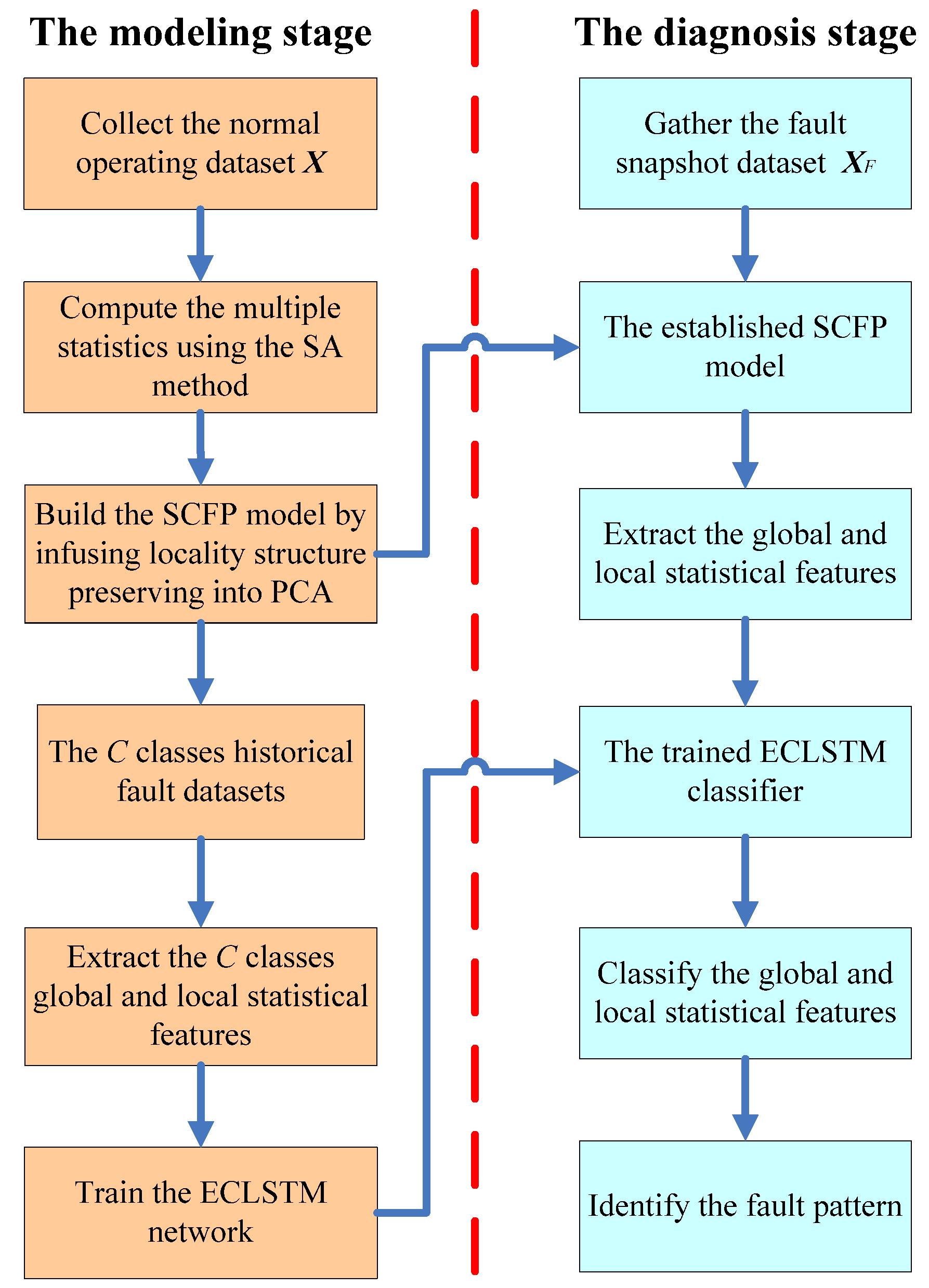
To diagnose the fault pattern of the transmission line, the first 500 collected fault samples are utilized to build the snapshot dataset. And the rest of the 500 fault samples from the same pattern are regarded as the historical fault dataset. The ECLSTM-based fault diagnosis model is first trained by feeding the mined historical fault datasets’ global and local statistical features, which are extracted by the developed SCFP approach, and the snapshot dataset’s global and local statistical features are then extracted and imported into the established ECLSTM-based diagnosis model for the purpose of identifying the pattern of the detected fault.

5.2. Compared Approaches and Effectiveness Evaluation Index

To testify the effectiveness of the proposed ECLSTM-based diagnosis approach, some traditional and closely related fault diagnosis methods, i.e., the support vector machine (SVM), the convolutional neural network (CNN), the deep belief network (DBN), and the long short-term memory (LSTM), are contrasted with the suggested ECLSTM. The global and local statistical features derived by the constructed SCFP are respectively fed to the SVM, CNN, DBN, and ELSTM. And these improved fault diagnosis methods are respectively termed the ESVM, ECNN, EDBN, and ELSTM.

To train the ECLSTM and ELSTM-based diagnosis models, the number of hidden units is set to 300, the batch size is 64, and the 0.001 learning rate is utilized with the help of cross-validation. In addition, the optimal model parameters are determined by the Adam optimizer. The node numbers of the ECNNs three convolution layers are respectively selected as 32, 64, and 128 by trial and error, while the neuron numbers in the EDBNs first, second, and third hidden layers are respectively 500, 300, and 200. Similar to the ECLSTM and ELSTM, the batch size and the learning rate in the ECNN and EDBN are also chosen as 64 and 0.001 for fairness. In the ESVM, the Gaussian kernel function is adopted, and the parameter is set to 600 by the grid search method. In addition, the weight factor of the ESVM is experientially determined at 50.

To assess the performance of the discussed ECLSTM for transmission line fault diagnosis, four performance indices, i.e., the fault diagnosis rate $FDR(i), i=1,2,\dots ,C$ of fault samples in the i-th pattern, the average fault diagnosis rate $FD{R}_{\mathrm{average}}$ of fault samples in the total of C patterns, the precision P(i), i = 1, 2, …, C for the i-th pattern, and the average precision, P_average are employed.

Particularly, the index $FDR(i)$ is defined as

$$FDR(i)=\frac{N_i(i)}{N_i}, i=1,\cdots ,C$$

(32)

where $N_i(i)$ denotes the number of correctly diagnosed fault samples for the i-th pattern.

The index $FD{R}_{\mathrm{average}}$ expressed in Equation (33) indicates the average value of all the acquired fault diagnosis rates for the C fault snapshot datasets.

$$FD{R}_{\mathrm{average}}=\frac{1}{C}{\displaystyle \sum _{i=1}^{C}FDR(i)}$$

(33)

The precision $P\left(i\right), i=1,2,\dots ,C$ for the i-th pattern is defined as

$$P(i)=\frac{N_i(i)}{(N_i(i)+F{P}_i(i))}$$

(34)

where $F{P}_i(i)$ represents the number of wrongly identified fault samples in the i-th pattern.

The index average precision $P_{\mathrm{average}}$ expressed in Equation (35) indicates the average value of all the computed precisions for the C fault snapshot datasets.

$$P_{\mathrm{average}}=\frac{1}{C}{\displaystyle \sum _{i=1}^{C}P(i)}$$

(35)

5.3. The Comparison of Accuracies for the Diagnosis Methods’ Training Process

The remaining 500 fault samples from each fault pattern are regarded as the historical fault dataset, i.e., the training dataset. The training process of the fault diagnosis network stops as the values of the FDR for the eleven training datasets are all above 98.00%. To reveal the accuracy of the diagnosis network during the training process, the 200 fault samples randomly selected from the historical fault dataset are adopted to construct a validation dataset for each short-circuit fault pattern. After the five fault diagnosis models are trained on the training datasets, the eleven validation datasets’ global and local statistical features are further inputted into these five trained models to figure out the accuracy of the training process.

The accuracies (i.e., the values of the FDR) of the ESVM, ECNN, EDBN, ELSTM, and ECLSTM-based diagnosis networks for the eleven fault patterns during the training process are revealed in

Table 2. The accuracies (values of the FDR) of the five fault diagnosis approaches during the training process.

Fault Pattern	ESVM	ECNN	EDBN	ELSTM	ECLSTM
AG	84.00%	95.00%	92.00%	93.50%	98.00%
BG	90.50%	87.50%	94.50%	93.50%	94.00%
CG	80.50%	81.00%	98.00%	94.00%	96.00%
AB	74.50%	71.50%	91.00%	87.50%	94.00C
BC	84.00%	98.50%	82.50%	86.50%	98.50%
AC	78.50%	84.50%	89.00%	96.50%	100.00%
ABG	83.50%	90.00%	87.00%	99.00%	96.50%
BCG	88.00%	94.00%	93.50%	99.00%	96.50%
ACG	95.50%	95.00%	100.00%	91.50%	99.50%
ABC	75.00%	90.50%	86.00%	91.50%	97.00%
ABCG	92.50%	86.50%	88.50%	100.00%	95.00%
FDRaverage	84.23%	88.55%	91.27%	93.86%	96.82%

. In addition, the values of the index $FD{R}_{\mathrm{average}}$ for the five diagnosis models during the training process are also given out. From Table 2, the values of the index $FD{R}_{\mathrm{average}}$ for the ESVM, ECNN, EDBN, ELSTM, and ECLSTM are respectively computed as 84.23%, 88.55%, 91.27%, 93.86%, and 96.82%. Thus, during the training process, the ECLSTM-based approach demonstrates the highest accuracy for all eleven fault patterns among the five approaches. What is more, in comparison with the ESVM, ECNN, EDBN, and ELSTM, the suggested ECLSTM also exhibits more remarkable diagnosis performance to discern the particular validation datasets of the eleven fault patterns in terms of the FDR values.

5.4. The Comparison of the Fault Diagnosis Results

(1) Fault diagnosis effectiveness verification of the proposed SCFP based feature extraction

In order to prove the improvement of the suggested statistics comprehensive feature preserving (SCFP) technique’s fault diagnosis performance, the SCFP-based feature extraction technique is compared with statistics analysis (SA), principal component analysis (PCA), and locality-preserving-based methods. In our work, the developed SCFP technique is combined with the CLSTM classifier to build the ECLSTM method. Similarly, the SA, PCA, and locality preservation are combined with the CLSTM classifier to respectively build the SCLSTM, GCLSTM, and LCLSTM approaches. In this way, the fault diagnosis capabilities of the SCFP, SA, global feature, and local feature-based exaction approaches can be analyzed.

The fault diagnosis results of the SCLSTM, GCLSTM, LCLSTM, and ECLSTM for the eleven fault patterns are listed in

Table 3. The values of the index FDR for the SCLSTM, GCLSTM, LCLSTM, and ECLSTM.

Fault Pattern	SCLSTM	GCLSTM	LCLSTM	ECLSTM
AG	89.60%	86.50%	83.80%	95.60%
BG	85.00%	82.80%	87.20%	90.80%
CG	90.00%	87.60%	85.40%	92.20%
AB	86.80%	84.40%	83.20%	91.80%
BC	93.60%	86.40%	96.40%	97.40%
AC	94.80%	87.20%	90.60%	98.00%
ABG	85.20%	77.20%	83.80%	93.40%
BCG	91.60%	85.60%	91.40%	94.80%
ACG	93.60%	90.80%	85.60%	98.20%
ABC	85.20%	82.00%	78.00%	92.60%
ABCG	87.60%	78.40%	81.60%	94.20%
FDRaverage	88.36%	84.45%	86.09%	94.45%

and

Table 4. The values of the index P for the SCLSTM, GCLSTM, LCLSTM and ECLSTM.

Fault Pattern	SCLSTM	GCLSTM	LCLSTM	ECLSTM
AG	87.00%	85.50%	83.80%	95.79%
BG	90.00%	84.80%	86.20%	93.80%
CG	85.20%	83.40%	85.80%	95.64%
AB	88.80%	81.00%	82.40%	94.25%
BC	85.80%	85.00%	90.60%	94.20%
AC	87.20%	86.80%	83.40%	92.45%
ABG	86.40%	83.20%	84.80%	95.50%
BCG	89.20%	87.20%	86.20%	93.86%
ACG	90.40%	88.40%	84.80%	95.34%
ABC	88.20%	85.80%	87.20%	95.07%
ABCG	86.00%	84.00%	85.80%	93.27%
Paverage	87.65%	85.01%	85.54%	94.47%

. According to the values of index FDR shown in Table 3, the index $FD{R}_{\mathrm{average}}$ values for the SCLSTM, GCLSTM, LCLSTM, and ECLSTM are respectively calculated as 88.36%, 84.45%, 86.09%, and 94.45%. Thus, the ECLSTM demonstrates the highest value of the index $FD{R}_{\mathrm{average}}$ for all eleven fault patterns. Anyway, in comparison with the SCLSTM, GCLSTM, and LCLSTM, the ECLSTM also exhibits more remarkable diagnosis performance to discern the eleven fault patterns in terms of the index FDR values. For example, for the fault pattern AC, the values of the index FDR for the SCLSTM, GCLSTM, LCLSTM, and ECLSTM are respectively calculated as 94.80%, 87.20%, 90.60%, and 98.00%, which proves that the ECLSTM owns the highest value of the index FDR among these four fault diagnosis models. Analogously, according to the values of precision P displayed in Table 4, the ECLSTM also reveals the highest value of the index P_average in comparison with the SCLSTM, GCLSTM, and LCLSTM. Furthermore, the ECLSTM shows much higher values of precision P than the other three methods in terms of identifying the eleven fault patterns. In summary, the above experiments prove the outstanding fault diagnosis performance of the suggested SCFP-based feature extraction techniques.

(2) Fault diagnosis effectiveness verification of the developed ECLSTM based diagnosis model

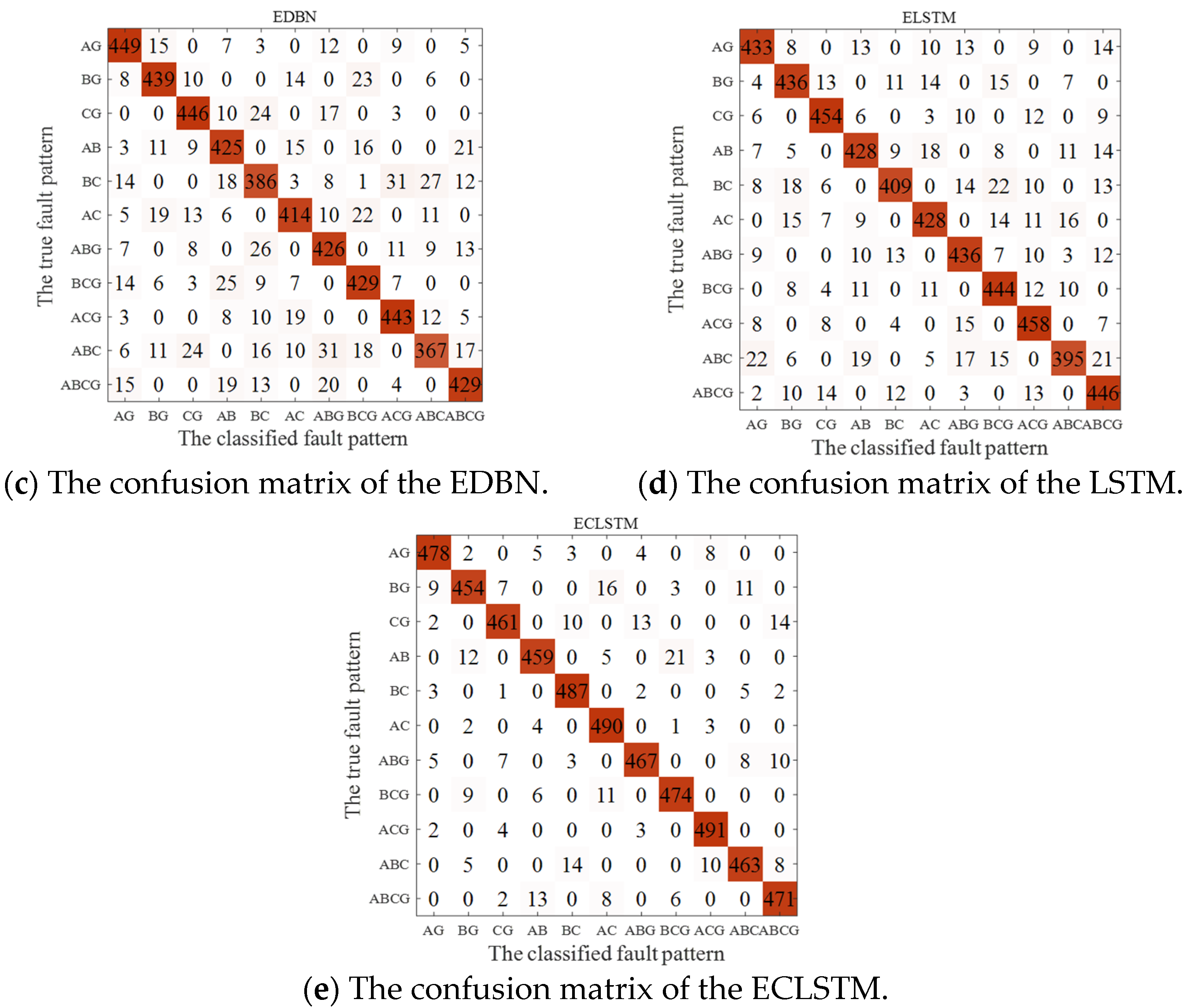
After the above-introduced eleven fault patterns are detected, the fault diagnosis rates of the ESVM, ECNN, EDBN, ELSTM, and ECLSTM for these eleven fault patterns are figured out and exhibited in Figure 4 and Figure 5. Specifically, Figure 4 gives out the confusion matrixes of these five fault diagnosis approaches. From Figure 4, the numbers in the dark orange blocks denote the numbers of accurately diagnosed fault samples, while the numbers in the shallow orange blocks stand for the numbers of mistakenly diagnosed fault samples. The orange block is darker, the number of fault samples is more. As displayed in Figure 4a–d, the numbers in the shallow orange blocks of the sixth rows for the ESVM, ECNN, EDBN, and ELSTM are much greater than those in Figure 4e of the ECLSTM. This demonstrates that more fault data points pertaining to the fault AC are mistakenly identified by the ESVM, ECNN, EDBN, and ELSTM. 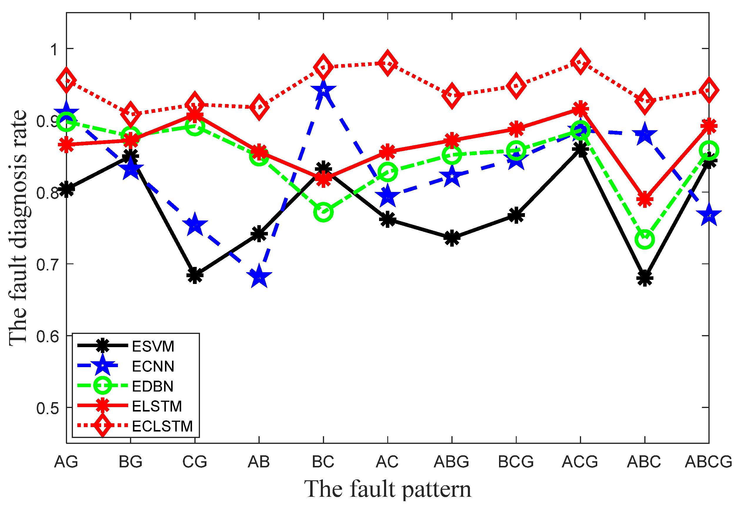Moreover, in comparison with Figure 4e, much more shallow orange blocks appear in Figure 4a–d. This phenomenon means that the ESVM, ECNN, EDBN, and ELSTM inaccurately discern much more fault data points for these eleven faults than the ECLSTM. To implement more graphical analysis and comparison, the line charts of the fault diagnosis rates for the five approaches under the eleven fault patterns are exhibited in Figure 5. As revealed in Figure 5, the fault diagnosis rates of the ECLSTM are significantly improved compared with those of the ESVM, ECNN, EDBN, and ELSTM. To be specific, the ECLSTMs values of the index FDR for the eleven fault patterns are all above 90.00%, and the fault diagnosis rate even reaches 98.20%. As displayed in Figure 5, the great differences between the fault diagnosis rates of the five approaches prove the superiority of the ECLSTM for implementing transmission line fault diagnosis.

The fault diagnosis rates of the ESVM, ECNN, EDBN, ELSTM, and ECLSTM for the eleven fault patterns are further quantized in

Table 5. The values of the index FDR for the five fault diagnosis approaches.

Fault Pattern	ESVM	ECNN	EDBN	ELSTM	ECLSTM
AG	80.40%	91.00%	89.80%	86.60%	95.60%
BG	85.00%	83.20%	87.80%	87.20%	90.80%
CG	68.40%	75.40%	89.20%	90.80%	92.20%
AB	74.20%	68.20%	85.00%	85.60%	91.80%
BC	83.20%	94.20%	77.20%	81.80%	97.40%
AC	76.20%	79.40%	82.80%	85.60%	98.00%
ABG	73.60%	82.20%	85.20%	87.20%	93.40%
BCG	76.80%	84.60%	85.80%	88.80%	94.80%
ACG	86.00%	88.60%	88.60%	91.60%	98.20%
ABC	68.00%	88.00%	73.40%	79.00%	92.60%
ABCG	84.40%	76.80%	85.80%	89.20%	94.20%
FDRaverage	77.84%	82.87%	84.60%	86.67%	94.45%

. In addition, for the sake of fairness, the values of the index $FD{R}_{\mathrm{average}}$ for the five diagnosis models on the eleven fault patterns are also exhibited in Table 5. From Table 5, the values of the index $FD{R}_{\mathrm{average}}$ for the ESVM, ECNN, EDBN, ELSTM, and ECLSTM are respectively computed as 77.84%, 82.87%, 84.60%, 86.67%, and 94.45%. Thus, the ECLSTM-based identification approach demonstrates the largest value of the index $FD{R}_{\mathrm{average}}$ for all eleven fault patterns among the five approaches, which testifies to the superiority of the ECLSTMs overall fault recognition effectiveness. What is more, in comparison with the ESVM, ECNN, EDBN, and ELSTM, the suggested ECLSTM also exhibits more remarkable diagnosis performance to discern the particular fault of the eleven fault patterns. For example, the index FDRs value for the fault pattern BCG is 94.80% for the ECLSTM, in contrast to only 88.80% for the ELSTM, 85.80% for the EDBN, 84.60% for the ECNN, and 76.80% for the ESVM. 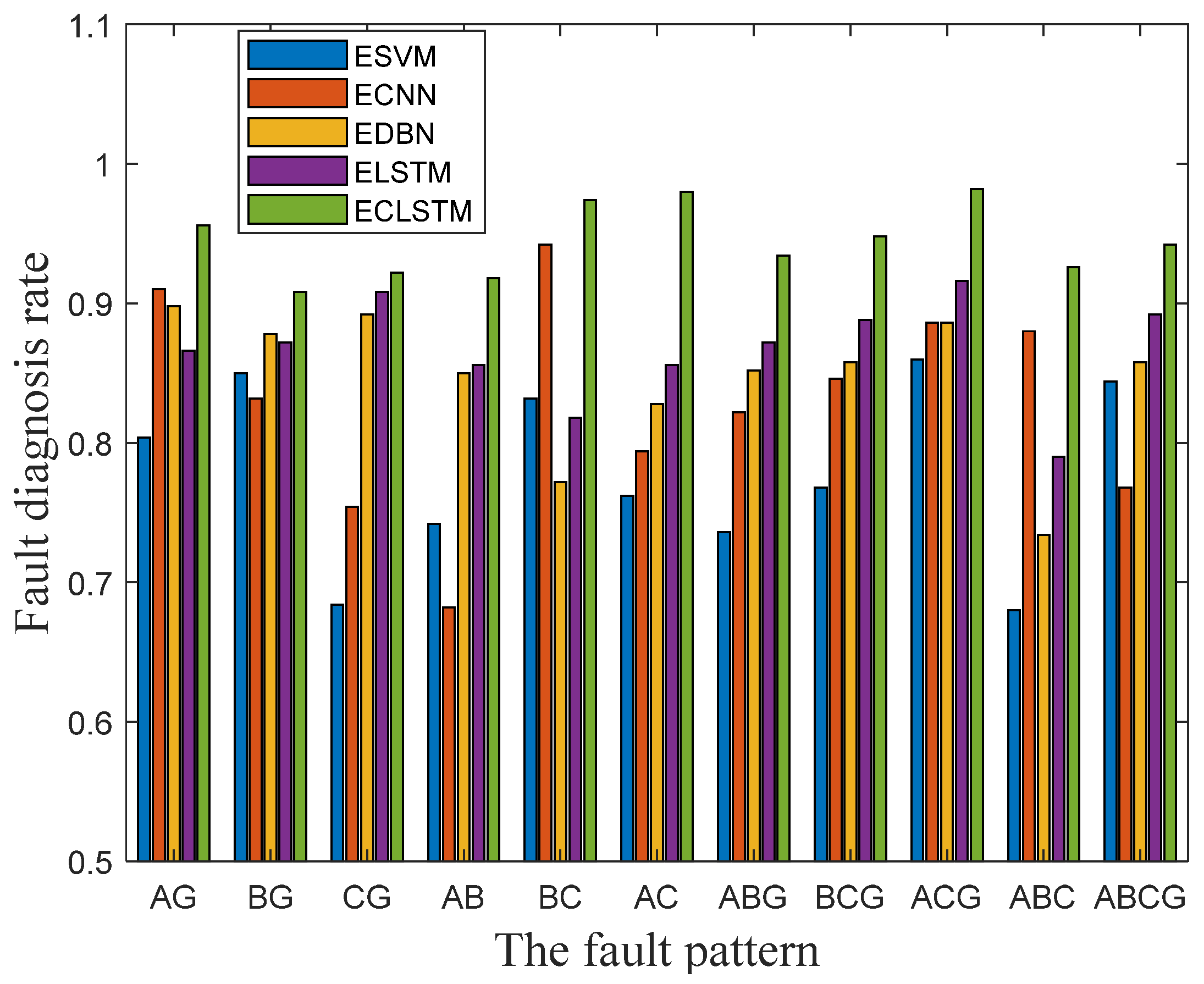Analogously, the value of the index FDR for the fault pattern AB is 91.80% for the ECLSTM, in comparison with only 85.60% for the ELSTM, 85.00% for the EDBN, 74.20% for the ESVM, and even 68.20% for the ECNN. It can be concluded that the presented ECLSTM approach is excellent for recognizing the short-circuit fault patterns of the transmission line. This is because the global and local statistical features extracted by the ECLSTM promote the improvement of the transmission line’s fault identification task. To facilitate further visualized analysis, the values of the index FDR for the five algorithms under the eleven fault patterns are plotted as the histogram in Figure 6, which also proves the outstanding recognition performance of the ECLSTM over the ESVM, ECNN, EDBN, and ELSTM for discerning all the eleven short circuit faults.

According to the confusion matrices given in Figure 4, the values of the index precision P for the ESVM, ECNN, EDBN, ELSTM, and ECLSTM are also listed in

Table 6. The values of the index precision P for the five fault diagnosis approaches.

Fault Pattern	ESVM	ECNN	EDBN	ELSTM	ECLSTM
AG	73.63%	82.13%	85.69%	86.77%	95.79%
BG	79.29%	80.15%	87.62%	86.17%	93.80%
CG	78.98%	87.07%	86.94%	89.72%	95.64%
AB	75.25%	83.17%	82.05%	86.29%	94.25%
BC	68.65%	80.93%	79.26%	89.30%	94.20%
AC	78.23%	81.35%	85.89%	87.53%	92.45%
ABG	76.03%	86.16%	81.30%	85.83%	95.50%
BCG	80.00%	83.76%	84.28%	84.57%	93.86%
ACG	82.69%	85.52%	87.20%	85.61%	95.34%
ABC	83.95%	83.97%	84.95%	89.37%	95.07%
ABCG	82.75%	78.37%	85.46%	83.21%	93.27%
Paverage	78.13%	82.96%	84.60%	86.76%	94.47%

. Anyway, the values of the index $P_{\mathrm{average}}$ for the five diagnosis models are also exhibited in Table 6. From Table 6, the values of the index $P_{\mathrm{average}}$ for the ESVM, ECNN, EDBN, ELSTM, and ECLSTM are respectively computed as 78.13%, 82.96%, 84.60%, 86.76%, and 94.47%. Thus, the ECLSTM-based identification approach demonstrates the largest value of the index $P_{\mathrm{average}}$ for all eleven fault patterns, which testifies the superiority of the ECLSTMs overall fault recognition effectiveness. In comparison with the ESVM, ECNN, EDBN, and ELSTM, the suggested ECLSTM displays more remarkable diagnosis performance to discern the particular fault of the eleven fault patterns. For example, the index precision’s value of the fault pattern CG is 95.64% for the ECLSTM, in contrast to only 89.72% for the ELSTM, 87.07% for the ECNN, 86.94% for the EDBN, and 78.98% for the ESVM. Analogously, the value of the index precision for the fault pattern ABG is 95.50% for the ECLSTM, in comparison with only 86.16% for the ECNN, 85.83% for the ELSTM, 81.30% for the EDBN, and even 76.03% for the ESVM. It can be concluded that the presented ECLSTM approach is excellent for recognizing the short-circuit fault patterns of the transmission line.

(3) Fault diagnosis effects of the proposed ECLSTM under different noise environments

To further verify the fault diagnosis effects of the proposed ECLSTM-based model under different noise environments, Gaussian noise with a zero mean and different variances is introduced to the monitored variables. The specific values of Gaussian noise’s different variances are set to be 0.1, 0.01, 0.001, and 0.0001 by experience. In this way, the ECLSTMs fault diagnosis effects under different noise environments are tested and displayed in

Table 7. The values of the index FDR for the ECLSTM under different noise environments.

Fault Pattern	Variance (0.1)	Variance (0.01)	Variance (0.001)	Variance (0.0001)
AG	93.40%	95.60%	97.00%	97.80%
BG	87.80%	90.80%	92.400%	91.60%
CG	89.80%	92.20%	94.200%	93.00%
AB	91.60%	91.80%	92.00%	93.20%
BC	95.60%	97.40%	98.400%	97.80%
AC	95.40%	98.00%	99.20%	100.00%
ABG	91.40%	93.40%	94.80%	96.40%
BCG	93.40%	94.80%	96.20%	97.00%
ACG	94.40%	98.20%	99.60%	99.60%
ABC	89.20%	92.60%	94.00%	96.00%
ABCG	90.80%	94.20%	95.00%	96.40%
FDRaverage	92.07%	94.45%	95.71%	96.25%

and

Table 8. The values of the index precision P for the ECLSTM under different noise environments.

Fault Pattern	Variance (0.1)	Variance (0.01)	Variance (0.001)	Variance (0.0001)
AG	94.40%	95.79%	96.40%	99.80%
BG	89.40%	93.80%	94.20%	95.60%
CG	93.40%	95.64%	97.40%	96.00%
AB	90.40%	94.25%	94.40%	96.80%
BC	91.20%	94.20%	96.60%	96.00%
AC	88.60%	92.45%	94.60%	96.20%
ABG	95.00%	95.50%	98.20%	98.20%
BCG	89.00%	93.86%	95.20%	97.80%
ACG	91.00%	95.34%	97.20%	99.40%
ABC	94.80%	95.07%	97.60%	96.00%
ABCG	91.00%	93.27%	94.80%	93.80%
Paverage	91.65%	94.47%	96.05%	96.87%

.

To be specific, Table 7 lists the ECLSTMs FDR and FDR_average values, and Table 8 exhibits the ECLSTMs indices P and P_average values for the eleven fault patterns, with the noise variance varying from 0.1 to 0.0001. When the value of noise variance is 0.1, which is the largest in our experiment, the ECLSTM achieves the worst fault diagnosis performance as the values of the FDR_average and P_average are both the smallest, i.e., 92.07% and 91.65%, respectively. However, the ECLSTMs values of FDR_average and P_average at the largest noise variance environment can be acceptable because they are both above 91.00%. With the decrease in noise variance, the ECLSTMs fault diagnosis effect becomes better and better. However, when the noise variance decreases from 0.001 to 0.0001, the diagnosis effectiveness of the ECLSTM improves slightly because the FDR_average only varies from 95.71% to 96.25% and the P_average only increases from 96.05% to 96.87%.

6. Conclusions

A novel ECLSTM fault diagnosis strategy based on the SCFP scheme is developed to identify the fault in the transmission line. To our best knowledge, we are the first to incorporate the global and local statistical feature extraction technique into the CLSTM to diagnose the transmission line’s fault. The other two contributions are expressed below. Firstly, a novel SCFP algorithm is proposed to deal with the dynamic coupling properties and mine the global and local structure features of the transmission line data. To be specific, the SA method is first applied to tackle the dynamic coupling properties of the transmission line by calculating multiple statistical features of the original process data. Then, the CFP-based dimension reduction technique is further developed to maintain the global and local structure information of computed multiple statistics during feature extraction by integrating the locality structure preservation approach into the PCA model. Secondly, the troublesome problem of identifying the fault in the transmission line is addressed. After the global and local statistical features of the snapshot dataset are caught by the established SCFP technique, an ECLSTM-based fault diagnosis method is suggested to classify these statistical features by considering the ECLSTMs capability to tackle the temporal dependencies and spatial correlations of the mined global and local statistical features. The detailed experiments certify the excellent fault diagnosis effect of the presented SCFP-based ECLSTM fault recognition strategy to diagnose the transmission line fault.

References

1. Rajesh, P.; Kannan, R.; Vishnupriyan, J.; Rajani, B. Optimally detecting and classifying the transmission line fault in power system using hybrid technique. ISA Trans. 2022, 130, 253–264. [Google Scholar] [CrossRef] [PubMed]
2. Liu, Y.; Lu, D.; Vasilev, S.; Wang, B.; Lu, D.; Terzija, V. Model-based transmission line fault location methods: A review. Int. J. Electr. Power Energy Syst. 2023, 153, 109321. [Google Scholar] [CrossRef]
3. França, I.A.; Vieira, C.W.; Ramos, D.C.; Sathler, L.H.; Carrano, E.G. A machine learning-based approach for comprehensive fault diagnosis in transmission lines. Comput. Electr. Eng. 2022, 101, 108107. [Google Scholar] [CrossRef]
4. Li, C.; Shen, C.; Zhang, H.; Sun, H.; Meng, S. A novel temporal convolutional network via enhancing feature extraction for the chiller fault diagnosis. J. Build. Eng. 2021, 42, 103014. [Google Scholar] [CrossRef]
5. Yaman, O.; Ertam, F.; Tuncer, T. Automated Parkinson’s disease recognition based on statistical pooling method using acoustic features. Med. Hypotheses 2020, 135, 109483. [Google Scholar] [CrossRef] [PubMed]
6. Yang, J.; Lv, Z.; Shi, H.; Tan, S. Performance monitoring method based on balanced partial least square and statistics pattern analysis. ISA Trans. 2018, 81, 121–131. [Google Scholar] [CrossRef]
7. He, Q.P.; Wang, J.; Shah, D. Feature space monitoring for smart manufacturing via statistics pattern analysis. Comput. Chem. Eng. 2019, 126, 321–331. [Google Scholar] [CrossRef]
8. You, L.X.; Chen, J. A variable relevant multi-local PCA modeling scheme to monitor a nonlinear chemical process. Chem. Eng. Sci. 2021, 246, 116851. [Google Scholar] [CrossRef]
9. Zhou, Y.; Xu, K.; He, F.; He, D. Nonlinear fault detection for batch processes via improved chordal kernel tensor locality preserving projections. Control. Eng. Pract. 2020, 101, 104514. [Google Scholar] [CrossRef]
10. He, Y.L.; Zhao, Y.; Hu, X.; Yan, X.N.; Zhu, Q.X.; Xu, Y. Fault diagnosis using novel AdaBoost based discriminant locality preserving projection with resamples. Eng. Appl. Artif. Intell. 2020, 91, 103631. [Google Scholar] [CrossRef]
11. Somayeh Mirzaei Kang, J.L.; Chu, K.Y. A comparative study on long short-term memory and gated recurrent unit neural networks in fault diagnosis for chemical processes using visualization. J. Taiwan Inst. Chem. Eng. 2021, 130, 104028. [Google Scholar]
12. Xing, Y.; Lv, C. Dynamic state estimation for the advanced brake system of electric vehicles by using deep recurrent neural networks. IEEE Trans. Industr. Electron. 2019, 67, 9536–9547. [Google Scholar] [CrossRef]
13. Zhang, Z.; Lv, Z.; Gan, C.; Zhu, Q. Human action recognition using convolutional LSTM and fully-connected LSTM with different attentions. Neurocomputing 2020, 410, 304–316. [Google Scholar] [CrossRef]
14. Belagoune, S.; Bali, N.; Bakdi, A.; Baadji, B.; Atif, K. Deep learning through LSTM classification and regression for transmission line fault detection, diagnosis and location in large-scale multi-machine power systems. Measurement 2021, 177, 109330. [Google Scholar] [CrossRef]
15. Moradzadeh, A.; Teimourzadeh, H.; Mohammadi-Ivatloo, B.; Pourhossein, K. Hybrid CNN-LSTM approaches for identification of type and locations of transmission line faults. Int. J. Electr. Power Energy Syst. 2022, 135, 107563. [Google Scholar] [CrossRef]
16. Haq, E.U.; Jianjun, H.; Li, K.; Ahmad, F.; Banjerdpongchai, D.; Zhang, T. Improved performance of detection and classification of 3-phase transmission line faults based on discrete wavelet transform and double-channel extreme learning machine. Electr. Eng. 2021, 103, 953–963. [Google Scholar] [CrossRef]
17. Palla, G.L.P.; Pani, A.K. Independent component analysis application for fault detection in process industries: Literature review and an application case study for fault detection in multiphase flow systems. Measurement 2023, 209, 112505. [Google Scholar]
18. Torres de Alencar, G.; Dos Santos, R.C.; Neves, A. A new robust approach for fault location in transmission lines using single channel independent component analysis. Electr. Power Syst. Res. 2023, 220, 109281. [Google Scholar] [CrossRef]
19. Gao, L.; Li, D.; Liu, X.; Liu, G. Enhanced chiller faults detection and isolation method based on independent component analysis and k-nearest neighbors classifier. Build. Environ. 2022, 216, 109010. [Google Scholar] [CrossRef]
20. Liu, L.; Liu, J.; Wang, H.; Tan, S.; Yu, M.; Xu, P. A multivariate monitoring method based on kernel principal component analysis and dual control chart. J. Process Control. 2023, 127, 102994. [Google Scholar] [CrossRef]
21. Zhu, A.; Zhao, Q.; Yang, T.; Zhou, L.; Zeng, B. Condition monitoring of wind turbine based on deep learning networks and kernel principal component analysis. Comput. Electr. Eng. 2023, 105, 108538. [Google Scholar] [CrossRef]
22. Lu, X.; Long, J.; Wen, J.; Fei, L.; Zhang, B.; Xu, Y. Locality preserving projection with symmetric graph embedding for unsupervised dimensionality reduction. Pattern Recognit. 2022, 131, 108844. [Google Scholar] [CrossRef]
23. Chen, Y.; Lv, Y.; Wang, X.; Li, L.; Wang, F.Y. Detecting traffic information from social media texts with deep learning approaches. IEEE Trans. Intell. Transport. Syst. 2018, 20, 3049–3058. [Google Scholar] [CrossRef]
24. Zhang, H.; Yang, W.; Yi, W.; Lim, J.B.; An, Z.; Li, C. Imbalanced data based fault diagnosis of the chiller via integrating a new resampling technique with an improved ensemble extreme learning machine. J. Build. Eng. 2023, 70, 106338. [Google Scholar] [CrossRef]
25. Sun, W.; Paiva, A.R.; Xu, P.; Sundaram, A.; Braatz, R.D. Fault detection and identification using bayesian recurrent neural networks. Comput. Chem. Eng. 2020, 141, 106991. [Google Scholar]
26. Zheng, G.X.; Chen, W.; Qian, Q.J.; Kumar, A.; Sun, W.F.; Zhou, Y.Q. TCM in milling processes based on attention mechanism-combined long short-term memory using a sound sensor under different working conditions. Int. J. Hydromechatronics 2022, 5, 243–259. [Google Scholar] [CrossRef]
27. Zhou, Y.Q.; Kumar, A.; Parkash, C.; Vashishtha, G.; Tang, H.S.; Xiang, J.W. A novel entropy-based sparsity measure for prognosis of bearing defects and development of a sparsogram to select sensitive filtering band of an axial piston pump. Measurement 2022, 203, 111997. [Google Scholar] [CrossRef]
28. Han, Y.; Ding, N.; Geng, Z.; Wang, Z.; Chu, C. An optimized long short-term memory network based fault diagnosis model for chemical processes. J. Process Control 2020, 92, 161–168. [Google Scholar] [CrossRef]
29. Nogas, J.; Khan, S.S.; Mihailidis, A. Fall detection from thermal camera using convolutional LSTM autoencoder. In Proceedings of the 2nd Workshop on Aging, Rehabilitation and Independent Assisted Living at IJCAI, Federated Artificial Intelligence Meeting, Stockholm, Sweden, 15–17 July 2018; pp. 1–4. [Google Scholar]
30. Chen, B.J.; Li, T.M.; Ding, W.P. Detecting deepfake videos based on spatiotemporal attention and convolutional LSTM. Inf. Sci. 2022, 601, 58–70. [Google Scholar] [CrossRef]
31. Yu, J.B.; Liu, X.; Ye, L. Convolutional long short-term memory autoencoder-based feature learning for fault detection in industrial processes. IEEE Trans. Instrum. Meas. 2021, 70, 3505615. [Google Scholar] [CrossRef]
32. Fathabadi, H. Novel filter based ANN approach for short-circuit faults detection, classification and location in power transmission lines. Int. J. Electr. Power Energy Syst. 2016, 74, 374–383. [Google Scholar] [CrossRef]
33. Farshad, M.; Sadeh, J. Fault locating in high-voltage transmission lines based on harmonic components of one-end voltage using random forests. Iran. J. Electr. Electron. Eng. 2013, 9, 158–166. [Google Scholar]
34. Mitra, S.; Mukhopadhyay, R.; Chattopadhyay, P. PSO driven designing of robust and computation efficient 1D-CNN architecture for transmission line fault detection. Expert Syst. Appl. 2022, 210, 118178. [Google Scholar] [CrossRef]
35. Abdullah, A. Ultrafast transmission line fault detection using a DWT-Based ANN. IEEE Trans. Ind. Appl. 2018, 54, 1182–1193. [Google Scholar] [CrossRef]
36. Shi, X.; Chen, Z.; Wang, H.; Yeung, D.Y.; Wong, W.K.; Woo, W.C. Convolutional LSTM Network: A machine learning approach for precipitation nowcasting. Adv. Neural Inf. Process. Syst. 2015, 28, 802–810. [Google Scholar]
37. Deng, X.G.; Tian, X.M.; Chen, S.; Harris, C.J. Nonlinear process fault diagnosis based on serial principal component analysis. IEEE Trans. Neural Netw. Learn. Syst. 2018, 29, 560–572. [Google Scholar] [CrossRef]
38. Valle, S.; Li, W.; Qin, S.J. Selection of the number of principal components: The variance of the reconstruction error criterion with a comparison to other methods. Ind. Eng. Chem. Res. 1999, 38, 4389–4401. [Google Scholar] [CrossRef]
39. Fahim, S.R.; Sarker, S.K.; Muyeen, S.M.; Das, S.K.; Kamwa, I. A deep learning based intelligent approach in detection and classification of transmission line faults. Int. J. Electr. Power Energy Syst. 2021, 133, 107102. [Google Scholar] [CrossRef]
40. Kundur, P. Power System Stability and Control; McGraw-Hill: New York, NY, USA, 2022. [Google Scholar]
Figure 1. The architecture of the CLSTM network [30,31].
Processes 11 02955 g001
Figure 2. The enhanced feature extraction based ECLSTM fault diagnosis strategy.
Processes 11 02955 g002
Figure 3. The implementation step of the ECLSTM based fault diagnosis scheme.
Processes 11 02955 g003
Figure 4. The confusion matrices of the ESVM, ECNN, EDBN, ELSTM, and ECLSTM.
Processes 11 02955 g004aProcesses 11 02955 g004b
Figure 5. Line chart of the index FDRs values for the five fault diagnosis approaches.
Processes 11 02955 g005
Figure 6. The identification results of the ESVM, ECNN, EDBN, ELSTM, and ECLSTM for the eleven fault patterns.
Processes 11 02955 g006