Investigation of the Effect of Side Arm Orientation of the T-Junction on Gas–Liquid Stratified Flow

Abstract

T-junctions are important structures used in a number of industries to separate gas and liquid. This work studied the effect of the orientation of the side arm on the separation efficiency using a computational fluid dynamics (CFD) approach, and a new mechanical model is developed based on force analysis to predict the liquid carryout threshold. Laboratory experiments from published works are used to verify the CFD simulation and the new model. In this work, the angle of the side arm to the horizontal plane, $\mathsf{\alpha }$, and the angle of the side arm to the main arm’s axial direction, $\mathsf{\beta }$, are investigated. The results show that with increasing $\mathsf{\beta }$, the liquid carryover threshold increases accordingly, demonstrating that the liquid can be more easily carried to the side arm, while the liquid-carrying performance in the side arm is not sensitive to the inclination angle, $\mathsf{\beta }$. Hence, in the new model, the inclination angle of is ignored. Experimental data are collected to validate the new model. The results show that this model can accurately predict the liquid carryover threshold, and the relative error is 4.16%.

1. Introduction

Today, multiphase pipe flow is an essential part of power and process industries, such as power plants, chemical processing, and petroleum production. To utilize energy efficiently, it is important to separate different phases according to their physical properties [1,2]. Hence, various separators and corresponding separation mechanisms have attracted the attention of many scholars in recent years [3,4,5].

In the oil and gas production process, the mixed fluids produced from a wellbore always contain gas, oil and water, so two- or three-phase flow can occur in the transportation pipeline. In order to separate different phases, some conventional separators can be used [6,7,8]. However, the configuration of conventional separators not only occupies considerable space, but could also be dangerous because of the entrainment phenomenon, so they are not suitable for use in off-shore platforms or for placement on the seabed. To address this problem, the T-junction is widely used during the process of off-shore oil and gas transportation as it has the advantages of a compact structure, a small size, cost-effectiveness, and long-term safety [9,10,11]. Therefore, to design and optimize the structure of T-junctions, it is of great importance to investigate and understand their separation characteristics and mechanisms.

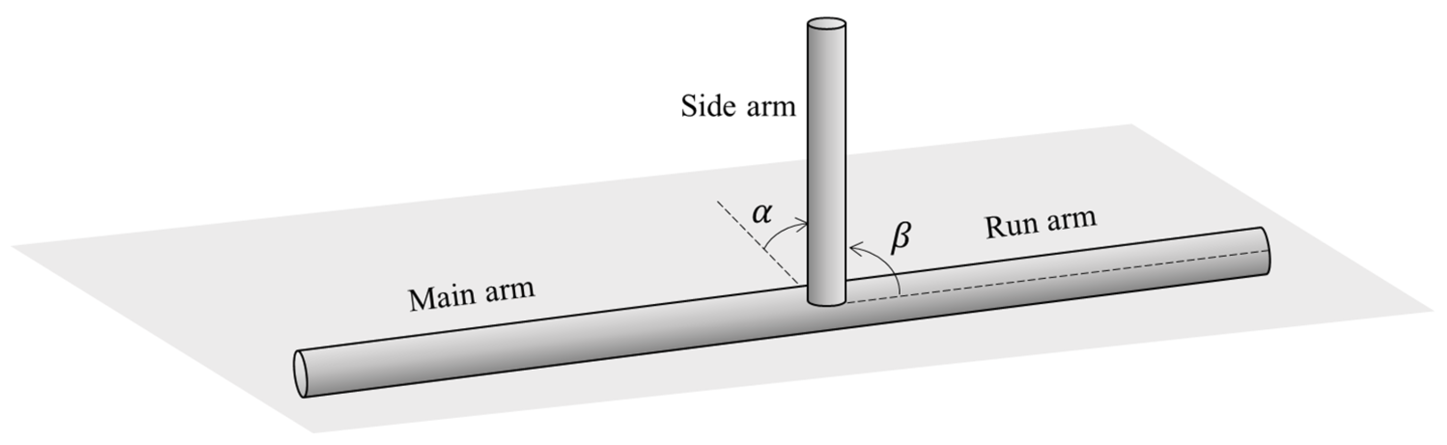
Figure 1 is a schematic of the T-junction, which consists of three parts: a main arm, a run arm, and a side arm. T-junctions can be classified into two categories according to the inflow condition [12]. If mixed fluids flow into the T-junction from the side arm, the mixture will hit the main pipe and then flow out via the main arm and run arm. In this case, the T-junction is called an impacting T-junction, whereas if the fluids are injected from the main arm, it is called a branching T-junction. In oil and gas transportation pipes, branching T-junctions are widely used. Therefore, this work focuses on a branching T-junction for gas and liquid separation. In Figure 1, there are two angles at which the orientation of the side arm is fixed: $\alpha$ and $\beta$. Here, $\mathsf{\alpha }$ is defined as the angle of inclination to the horizontal plane, while $\mathsf{\beta }$ is the angle of inclination to the axial direction of the main arm. If both $\alpha$ and $\beta$ are set to 90°, the side arm is positioned vertically to the horizontal plane.

In recent decades, numerous studies investigating the characteristics of the T-junction have been published. Hong [13] studied the effects of gas flow rate, liquid flow rate, and liquid viscosity on separation efficiency using a branching T-junction. It was found that the two-phase gas–liquid flow rate in the inlet pipeline has a significant impact on phase distribution. With the increase in inlet liquid velocity and decrease in inlet gas velocity, the amount of liquid extracted from the branch pipe is decreased. Moreover, it was reported that the phase separation in the T-junction is controlled by three forces: gravity, centripetal force, and inertial force. A change in the direction of gas entering the side arm generates significant centripetal force, which creates low pressure at the bend and pulls liquid into the branch pipe. If the gas flow rate is small, the centripetal force is reduced, and the difference in pressure decreases accordingly. Additionally, if the liquid flow velocity is relatively high, the inertia of the liquid phase is significant, and it is easy for liquid to flow along the main pipe and discharge via the run arm. This phenomenon has also been observed by other scholars [14], so it is generally accepted that gravitational, centripetal, and inertial forces dominate phase separation.

The mechanism reported by Hong [13] provides a simple description of the underlying physical behavior of a T-junction. However, deeper investigations of T-junctions are still a challenge considering T-junctions have various structures. Therefore, numerous studies of T-junctions have been carried out in recent decades. In particular, the research team lead by Azzopardi at Harwell laboratory carried out a large number of experiments to study the separation characteristics of gas and liquid in T-junctions. They systematically studied the influences of inlet flow regime [15,16,17], flow rate [18], inlet phase fraction [19], diameter ratio, and branch direction [20,21] on T-junctions. Across these studies, the diameter ratio of the side arm to the main arm has been treated as an important geometric parameter for phase separation.

Shoham et al. [22] studied the flow regimes of stratified and annular flows in T-junctions with the diameter ratios of 1.0 and 0.49. It was found that in both flow regimes, a smaller diameter ratio results in better phase separation. Wren [23] also found a similar phenomenon by studying the maldistribution of stratified and annular gas and liquid flows under 1.0 and 0.6 diameter ratio conditions. Griston and Choi [24] studied the phase separation performance of 1.0, 0.67, and 0.50 diameter ratio T-junctions. They reported that the reduced T-junctions have much less liquid carryover with smaller diameter ratios. It should be noted that the fluid medium in their experiment was wet steam; so, regardless of the properties of the operation fluid, reducing the diameter ratio of a T-junction can improve gas and liquid separation. Recently, Saieed [25] et al. investigated the influence of diameter ratio on gas–liquid separation in stratified flow and slug flow using laboratory experiments. In their study, five diameter ratios ranging from 1 to 0.2 were considered. They reported two parameters to describe the liquid carryover capacity in the side arm: liquid carryover threshold and liquid peak carryover. It was claimed that the liquid carryover threshold should be large and the liquid peak carryover should be small to mitigate the amount of liquid entering the side arm. They found that with a decrease in diameter ratio both of these parameters decreased. Although the liquid carryover threshold dropped with the diameter ratio, it was still high enough to deliver reasonable phase separation. So, they concluded that a reduction in diameter ratio always improves phase maldistribution.

In addition to the diameter ratio, the inclination angle of the side arm is another crucial parameter for phase separation. Yang et al. [26] found that the inclined angle of the side arm has a significant influence on the separation efficiency when the angle ranges from 0 to 30°. They claimed that that the separation performance increased with the increase in the angle. Penmatcha et al. [27] studied the influence of the side arm angle on the stratified gas and liquid flow, where the angle was set from +35° above the horizontal to −60° below. The results showed that more liquid can be carried to the side arm by increasing the downward inclination, and the majority of the gas phase can flow into the side arm with an increase in upward inclination.

However, the effect of side arm orientation on gas and liquid separation has not been fully revealed. The studies of inclination angle mentioned above focused on the deviated degree from the horizontal plane, which means the side arm is always placed vertically to the axial direction of the main pipe. To design a T-junction on off-shore platforms or on the seabed, the construction space is a dominant factor that should be taken into consideration, and so the orientation of the side arm should be carefully determined to reach the criteria of high separation efficiency and small size. Moreover, to help construction in the field, a model that can predict the critical status of liquid carryover in the side arm is still needed.

This paper aims to propose a new model to predict the liquid carryout threshold, which is helpful in designing T-junctions. Before developing the model, a CFD simulation is carried out and the properties of the T-junction are discussed; this will be presented in Section 2. Then, the new model will be established in Section 3. Experimental datasets are used to evaluate the accuracy of the proposed new model.

2. Effect of Side Arm Orientation

In this section, the effect of the side arm orientation is investigated using a CFD simulation approach. The simulation results will show how the orientation of the side arm affects the liquid-carrying capacity.

2.1. Numerical Method and Simulation Settings

Along with the development of high-performance computation technology, computational fluid dynamics (CFD) is becoming a powerful approach for modelling phase separation in T-junctions and predicting the flow properties. Lu et al. [3] carried out a comprehensive review of numerical studies of T-junctions. They reported that the Eulerian–Eulerian model and the VOF (volume of fluid) model have already been extensively applied in T-junctions, achieving great performance in gas and liquid separation simulations. Generally, the Eulerian–Eulerian model is useful for describing continuous two-phase flow by assuming that gas and liquid flows are continuous and interpenetrate one another, while the VOF model is designed to accurately capture the gas and liquid interface. In the Eulerian–Eulerian framework, there are two types of model: the two-phase model and the mixture model. Zhang et al. [28] compared the performance of the two models in a T-junction. It was found that the mixture model is better for modelling phase separation in the T-junction. Hence, in the present study, the mixture model is adopted. To clarify the simulation method and settings concisely, conservative equations of the mixture model, as well as the turbulence model, are presented in Appendix A. In this work, the simulation is carried out via the commercial software Fluent 19.0, released by the ANSYS company, San Diego, CA, USA.

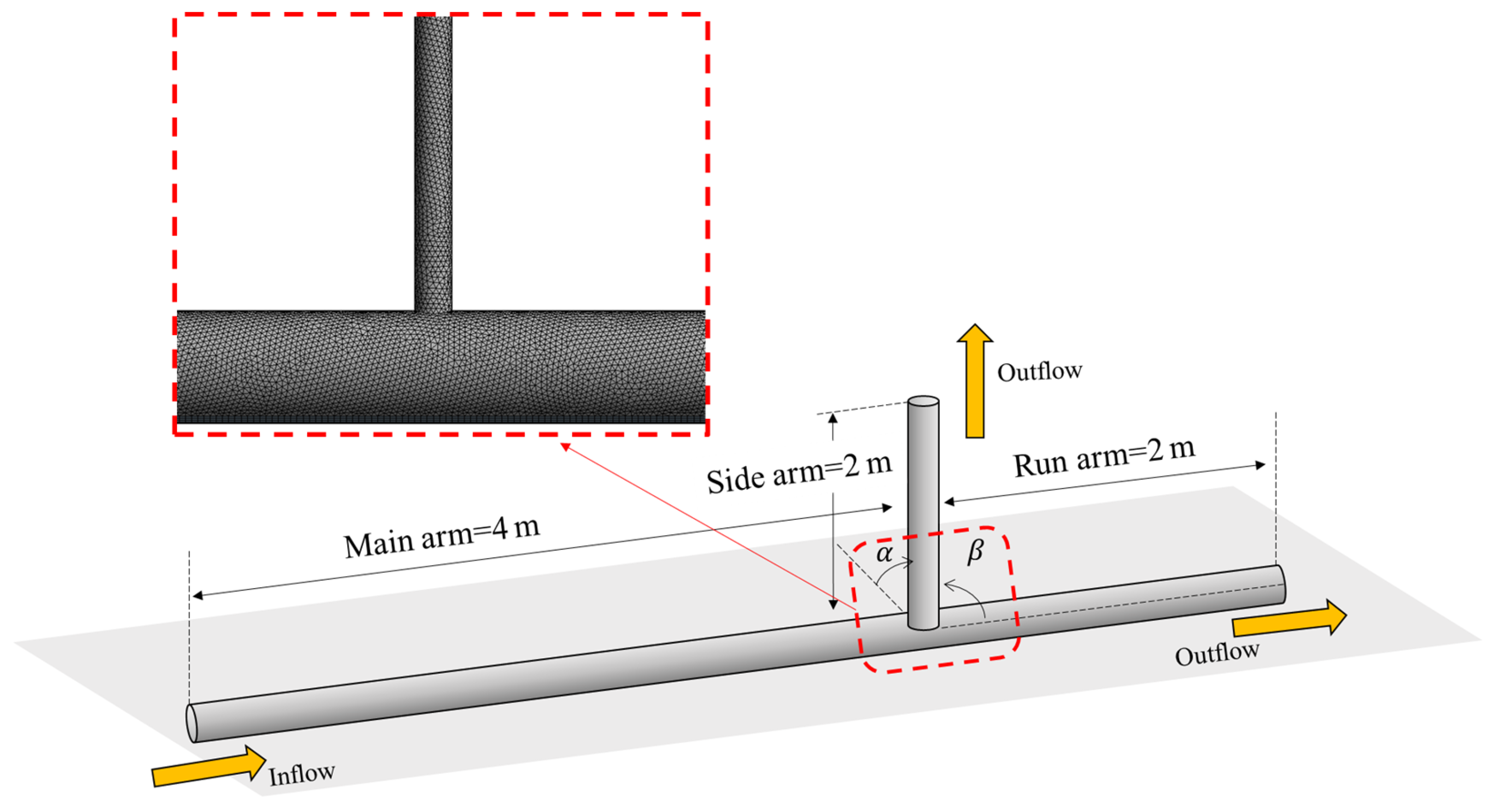
To investigate the effect of side arm orientation, an experimental case is required, and experimental data are needed to verify the simulation framework. Saieed et al. [25] carried out experiments to investigate the diameter ratio of a T-junction and provided comprehensive experimental parameters and datasets. Hence, this work adopted their experiment as the simulation reference. Figure 2 presents the simulation geometry based on Saieed et al.’s [25] experimental setup, where the diameters of the main arm and run arm are 0.078 m and the diameter of the side arm is 0.052 (diameter ratio = 0.67). The length of the main arm is set to 4 m, so the gas and liquid can be fully developed before they flow into the T-shape region. The lengths of the side arm and the run arm are both 2 m.

An unstructured mesh was produced for the geometric model, and a mesh study was carried out to determine a suitable mesh that can output reliable results within an acceptable simulation time. Three categories of mesh were tested to find a mesh that could produce accurate results within an acceptable computational time. In this work, the mesh was determined to be 1.21 × 10⁶ cells. Figure 2 displays a partial view of the generated mesh at the T-shape area.

In the simulation, air and water are selected as the two-phase medium. A velocity inlet condition was adopted, and the superficial velocities of gas and liquid were set to 0.178 m/s and 0.134 m/s, respectively. An outflow condition was adopted for the outlet boundary condition. It should be noted that there were two outflow boundaries: one for the side arm and one for the run arm. The flow rate of the side arm and the run arm can be changed by tuning the flow rate weighting parameter. This parameter is defined as the fractional flow rate through each boundary. In the current simulation, the flow rate weighting at the side arm was set to 0.3, 0.4, 0.5, 0.6, 0.7, and 0.8, which means that the percentage of the mixture flow in the side arm was 30%, 40%, 50%, 60%, 70%, and 80% to the total flow rate. Considering that water is the dominant phase in T-junctions, the liquid phase was set as the primary phase, and the pipe was full of liquid initially.

2.2. Evaluation of the CFD Simulation Results

Saieed et al.’s [25] experimental results are used to qualitatively and quantitatively evaluate the CFD simulation. In their work, one important parameter was used to quantify liquid-carrying performance: liquid carryout threshold. This is defined as the minimum fraction of gas in the side arm when the liquid begins to enter it. They claimed that in order to ensure less liquid enters the side arm, the liquid carryover threshold should be sufficiently large.

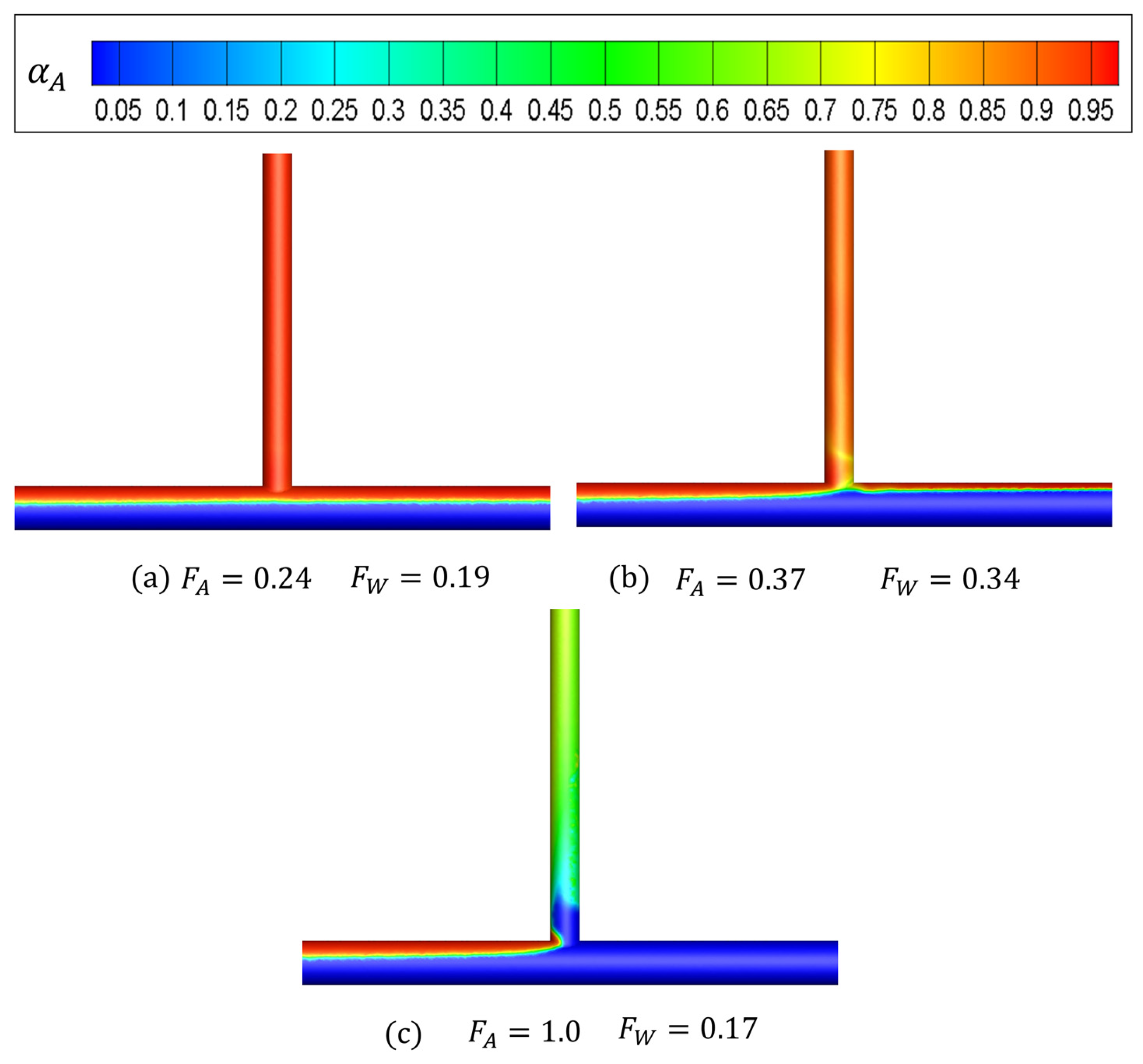
Figure 3 displays the phase fraction of air, ${\alpha }_A$, when the flow rate weighting of the side arm equals 0.3, 0.5, and 0.7. Here, ${\alpha }_A=1$ means pure air, while ${\alpha }_A=0$ implies pure water. Correspondingly, the gas flow rate portion, $F_A$, and the liquid flow rate portion, $F_W$, are also presented. $F_A$ is defined as the ratio of gas phase in the side arm to the main pipe, and $F_W$ denotes the ratio of liquid phase in the side arm to the main pipe. It is clear in Figure 3a, where the gas portion in the side arm is small, that there is no liquid in the side arm, hence the stratified flow is relatively stable in the main pipe. With the increase in the gas fraction in the side arm, the liquid is more likely to enter the side pipe. It can be seen in Figure 3b that a small amount of water flows into the side arm, corresponding to the liquid carryover threshold. Then, in Figure 3c, all gas is separated into the side arm. Meanwhile, more liquid is carried out to the side arm, forming an intermittent flow pattern.

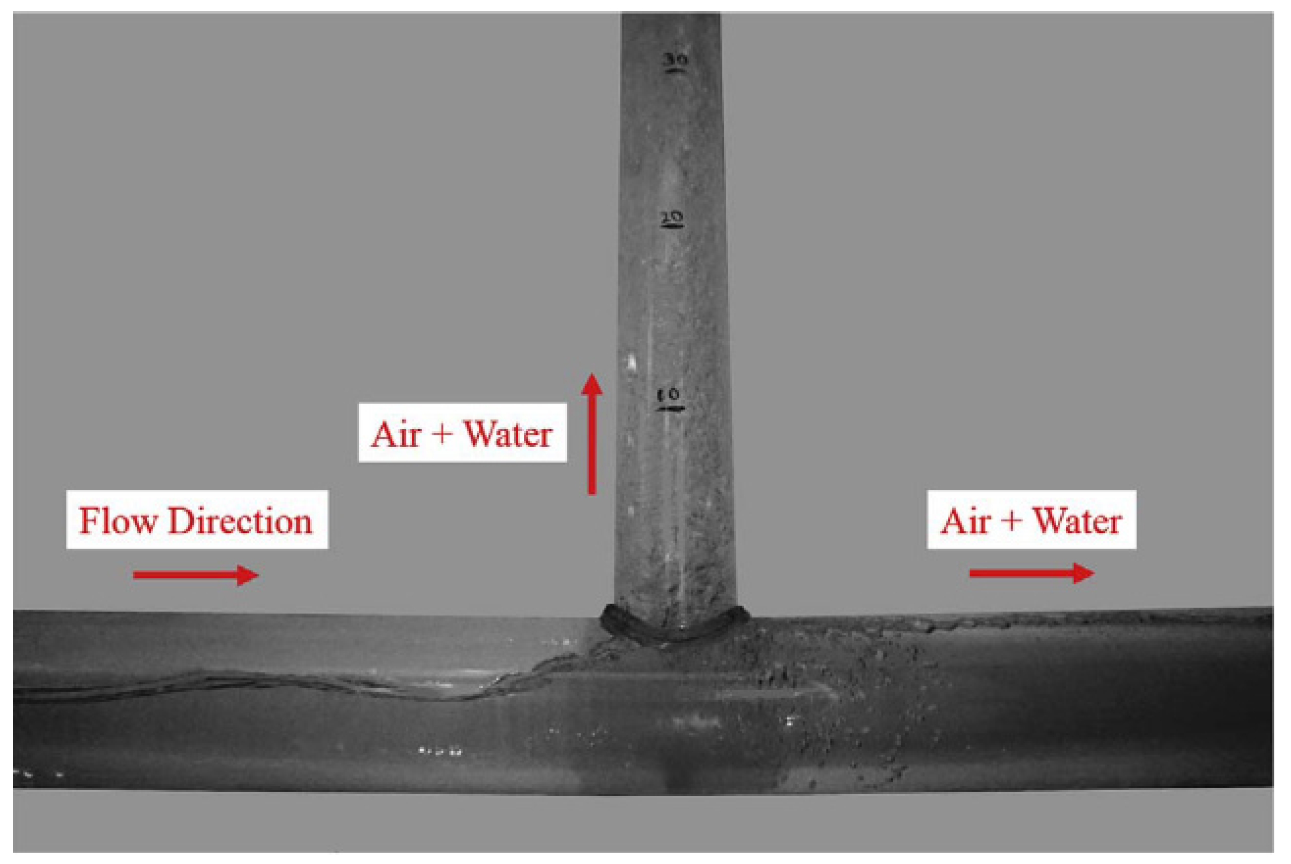
Figure 4 is a visual observation of the status of the liquid carryout threshold from Saieed et al.’s [25] experiment. It is clear that Figure 3b matches the experimental results qualitatively. The water level in the run arm is relatively high and some liquid is carried to the side arm. The two-phase flow in the side arm is relatively intermittent and chaotic. However, one discrepancy can be observed between experiment and simulation. In Figure 4, it is clear that there are entrainment behaviors in the T-junction. In the side arm, the dispersed droplets are entrained to the continuous gas phase. In the run arm, the dispersed bubbles exist in the continuous liquid phase. While, in Figure 3b, the entrainment process is not significant. This can be contributed to the fact that the entrainment is ignored in the CFD simulation. As presented in Section 2.1, the mixture model is adopted, which means that the two-phase flow is simulated in the average framework. To take the entrainment process into consideration, additional closure models should be introduced to the conservation equations. However, the entrainment behavior in the T-junction is too complicated to develop a reliable closure correlation based on the physical mechanisms. Hence, the gas and liquid entrainment behaviors are ignored in the CFD simulation.

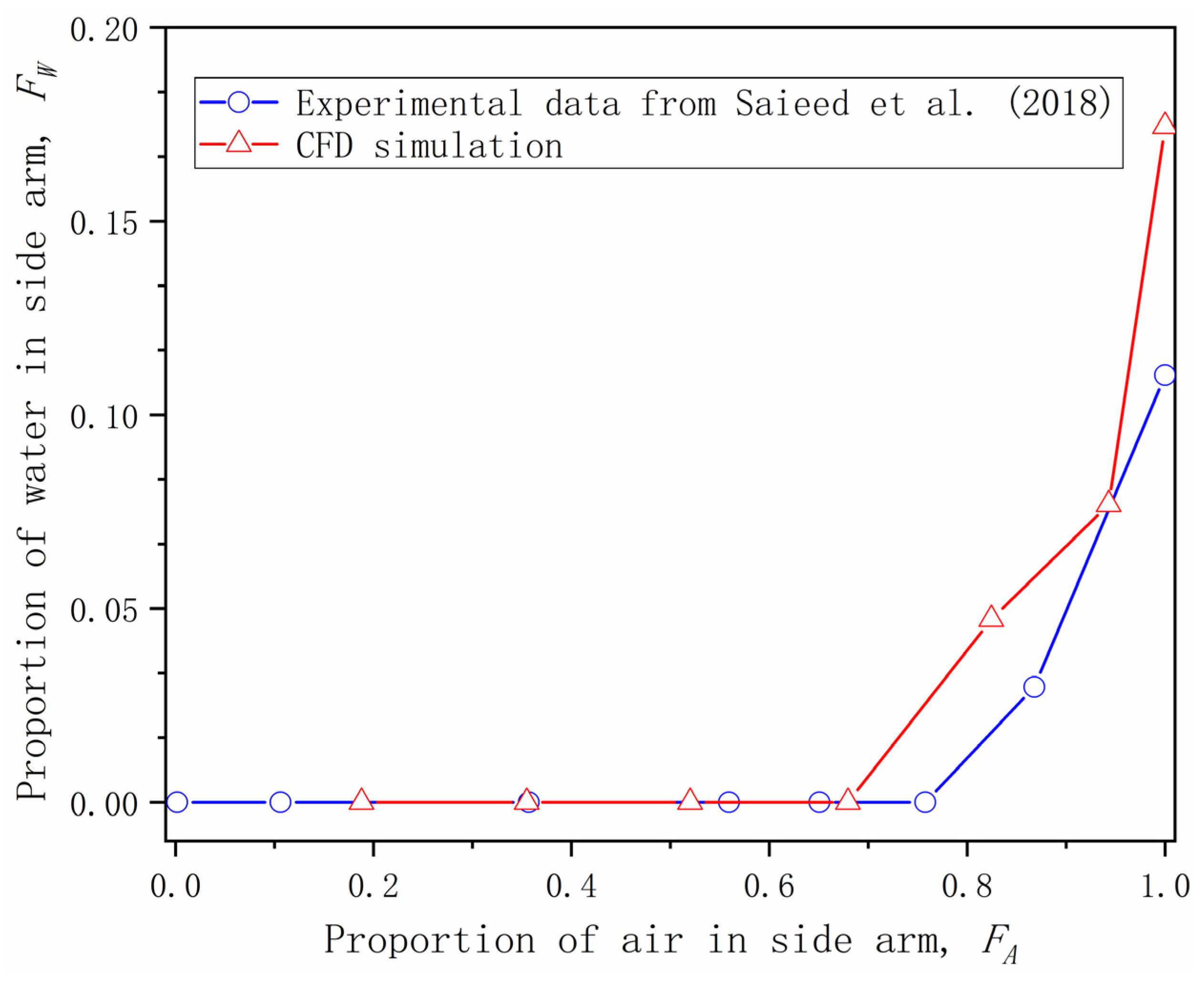
Figure 5 plots the liquid portion $F_W$ quantitatively at various gas portions $F_A$ based on the experiment and CFD simulation. It shows that the results of the CFD simulation are slightly higher than those of the experiment, which means that more liquid is carried to the side arm at the same gas fraction. Despite these discrepancies, the trend and order of magnitude in the CFD simulation are consistent with the experimental data. According to these results, one obvious conclusion can be drawn: the CFD simulation qualitatively matches the experimental results. However, in the quantitative comparison, the CFD simulation matches the experimental datasets in terms of trend and magnitude, but not specific numerical values. This could be attributed to the complicated nature of phase separation in the T-junction. In reality, the physical mechanisms of gas and liquid separation are relatively complex and involve gas and liquid divergence and entrainment properties. These characteristics mean that it is relatively difficult to simulate phase separation accurately in T-junctions. However, it should be noted that the goal of the CFD simulation was to understand the qualitative effect of the orientation, providing a basis for the following established model, rather than to calculate precise values that quantify phase separation. Hence, good simulation performance in terms of qualitative results and magnitude has been achieved in this work.

2.3. Parametric Study of Angle $\alpha$

In this subsection, the liquid carryout performance at an $\alpha$ of $0°$, $30°$, $45°$, $60°$, and $90°$ is investigated. To ignore the effect of $\beta$, the side arm was fixed vertically to the axial direction of the main pipe ($\beta =90°$).

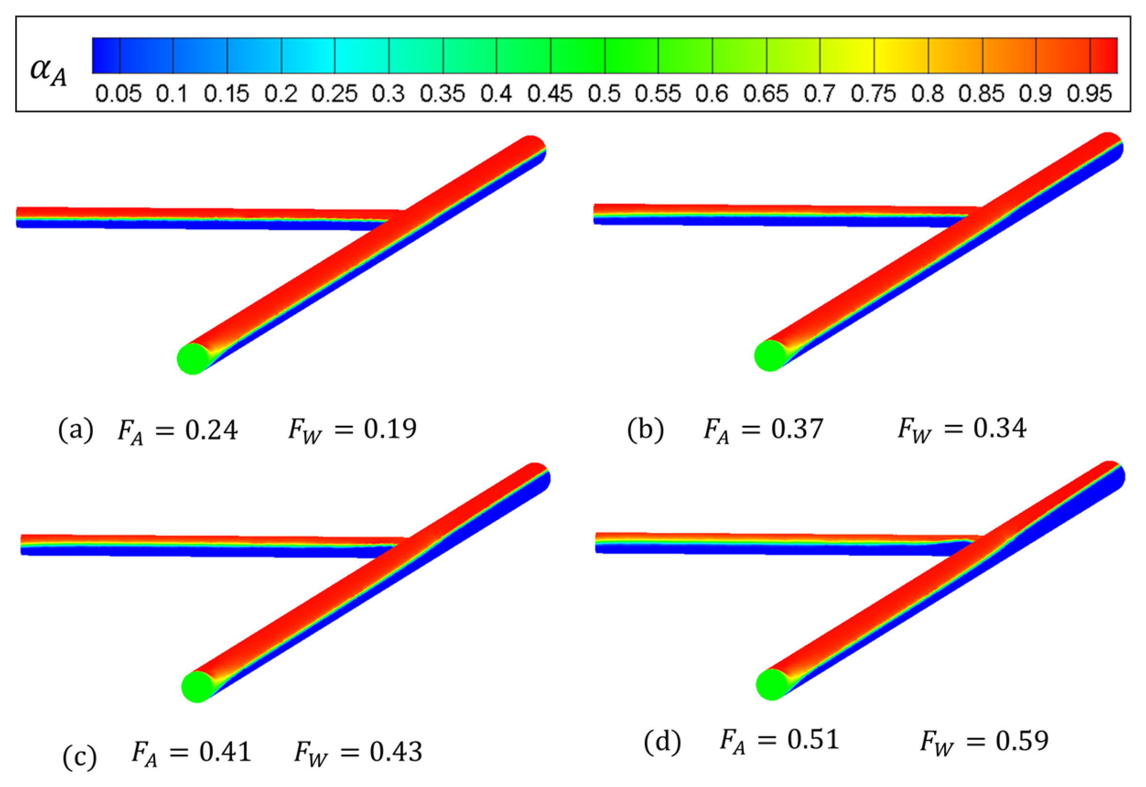
Figure 6 presents the phase fraction of air when $\alpha =0$ and the side arm is placed on the horizontal plane. It shows that the liquid flows into the side arm directly, and with the increase in $F_A$ in the side arm, more liquid is carried. This situation occurs when the diameter ratio, $D_s/D$, is large, and so the water level is high enough to submerge the side arm and then liquid can enter it directly. In this case, the liquid carryout threshold is zero since liquid flows to the side arm naturally. However, if the $D_s/D$ is so small that the water level in the main pipe is not high enough to submerge the side arm, the T-junction at $\alpha =0$ is available to completely separate the gas.

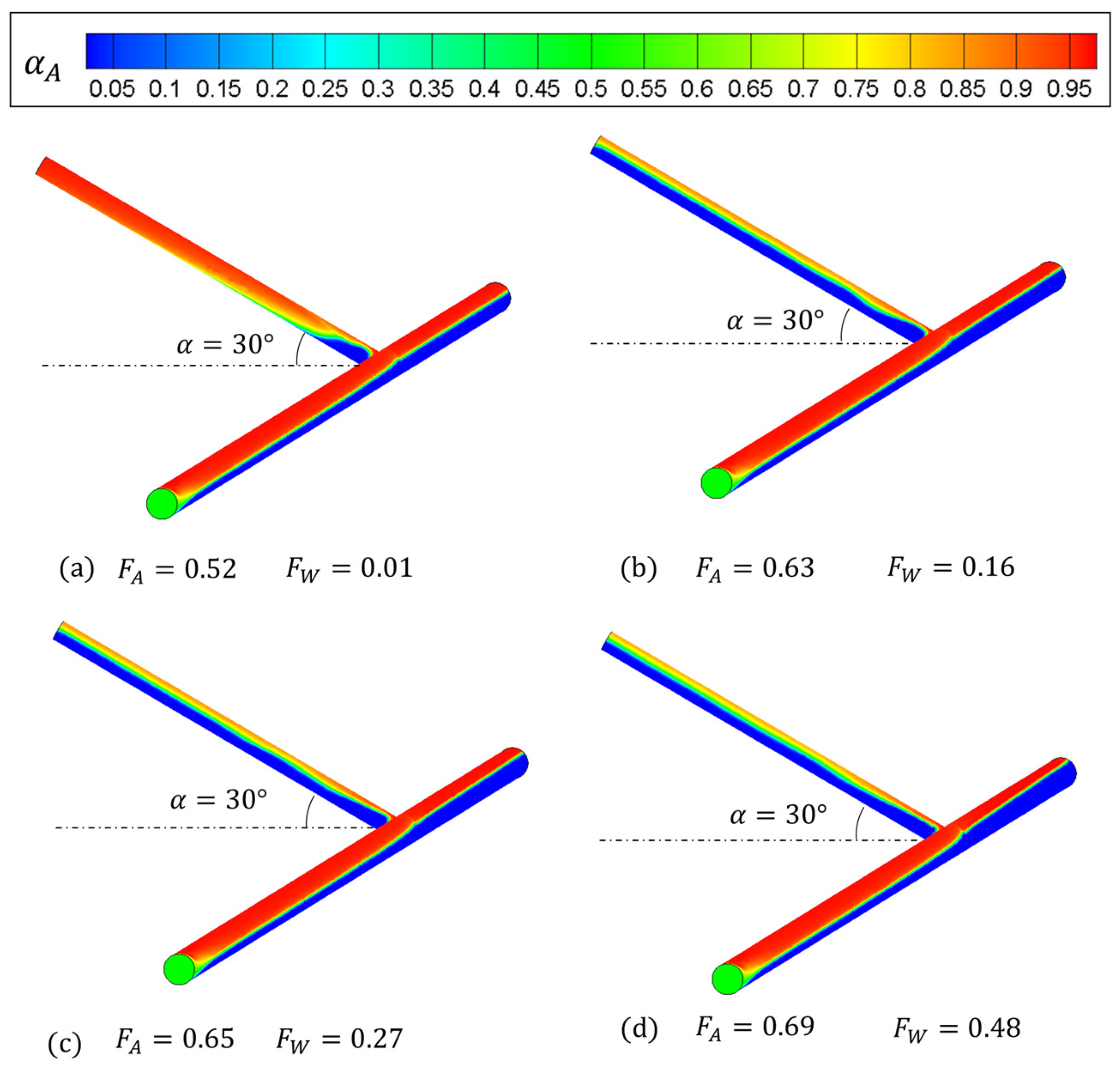
Figure 7 displays the gas fraction of the T-junction at $\alpha =30°$. When the gas fraction in the side arm is 0.52, the liquid enters the side arm directly, as shown Figure 7a. However, because of gravity the liquid in the side arm cannot completely flow out, which means that most of it returns to the main pipe. This phenomenon reveals that the gas flow rate in the side arm is not enough to carry the liquid flow upward. Then, with the increase in $F_A$, more liquid is carried into the side arm and a stratified flow pattern emerges. It can be seen in Figure 7b–d, where the $F_A$ is high enough to carry the liquid phase through the side arm, interfacial waves occur near the T-shape region, which could be caused by the disturbance of the gas and liquid in the T-junction. Another important phenomenon in Figure 7d is that there is a sucking effect from the stratified flow in the T-shaped region caused by the centripetal force.

Figure 8 shows the simulation results when $\alpha =45°$. In Figure 8a, where the gas fraction in the side arm is small, it is observed that a small amount of liquid is carried into the side arm, Then, with the increase in $F_A$, a stratified flow with interfacial waves develops gradually. A similar phenomenon can be seen in Figure 9, where $\alpha =60°$. Compared with Figure 8, it is more difficult for the liquid phase in Figure 9 to be carried. This is caused by the T-junction in Figure 9 being closer to the vertical direction, so there is more gravity in the side arm to suppress the liquid carryover.

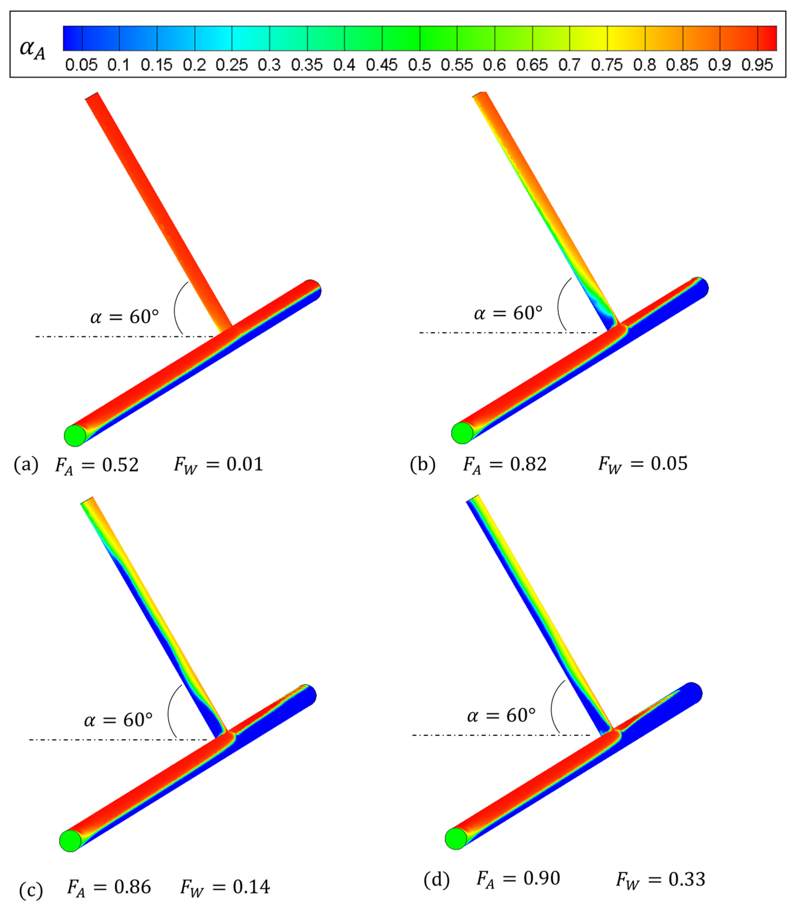
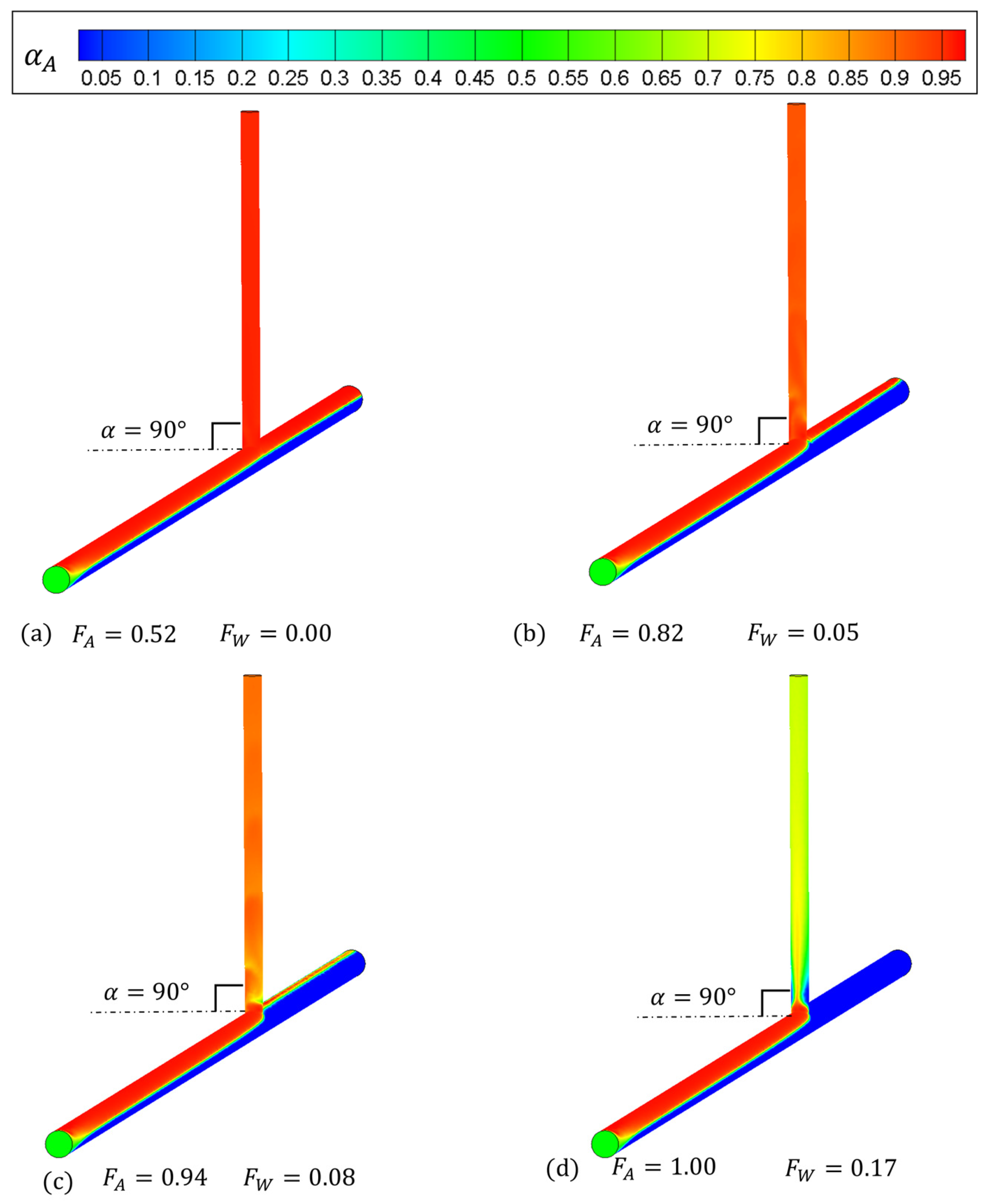
Figure 10 displays the CFD simulation when $\alpha =90°$, meaning that the T-junction is placed vertically on the horizontal plane. It can be seen in Figure 10a that no liquid enters the side arm. Then, in Figure 10b,c, it is observed that the sucking effect in the T-shape region is enhanced with the increase in $F_A$, so more liquid is carried. In Figure 10d, the gas and liquid two-phase flow in the side arm is relatively chaotic, and the flow pattern can be recognized as intermittent flow.

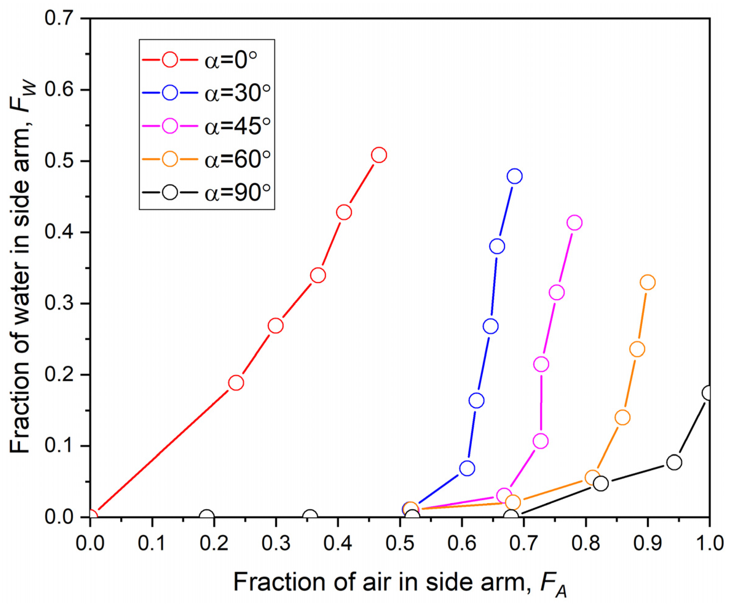
Figure 11 plots $F_W$ versus $F_A$ at different inclination angles from the horizontal plane, $\mathsf{\alpha }$. It is clear that $\mathsf{\alpha }$ has great influence on the liquid carryover capacity in the side arm. With the increase in $\mathsf{\alpha }$, a higher gas rate is required to carry the liquid to the side arm, so the liquid carryover threshold becomes larger with a larger $\mathsf{\alpha }$.

2.4. Parametric Study of Angle $\beta$

In this subsection, the inclination angle of $\beta$ is set to $30°,45°,\mathrm{and}60°$ to study the effect of the inclination angle of the side arm to the axial direction, while $\mathsf{\alpha }$ is fixed at $90°$.

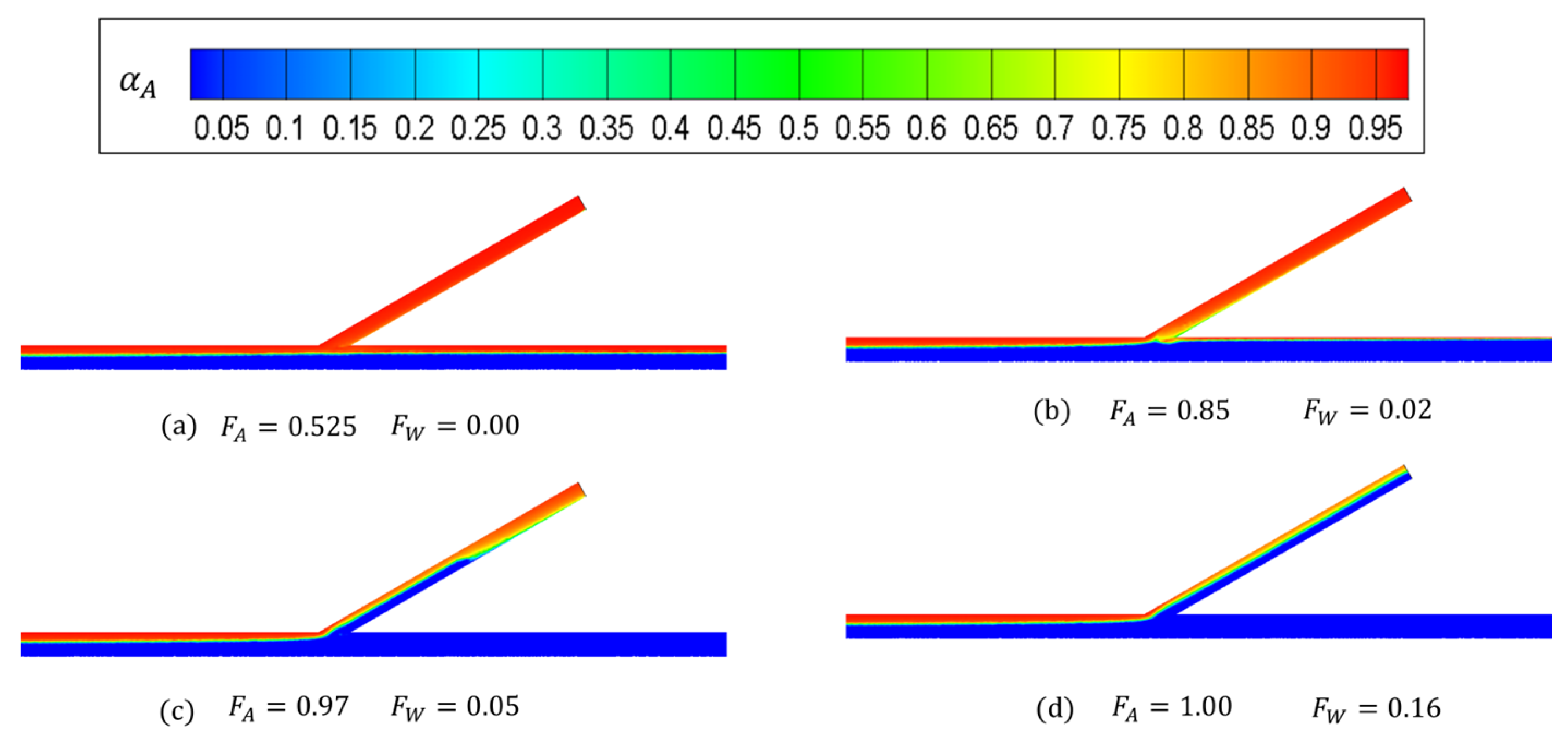
Figure 12 presents the phase fraction of air at $\beta =30°$. It can be seen that when $F_A=0.52$, the phase distribution in the T-junction is identical to that in Figure 10a; hence, changing the angle of $\beta$ does not help the liquid carryover. In Figure 12b–d, with the increase in $F_A$, it can be seen that a stratified flow develops gradually. This is different from Figure 10d, where the flow pattern is intermittent. Figure 13 and Figure 14 display a similar phenomenon to that in Figure 12. It is found that the angle,$\beta$, has little impact on the liquid carryover in the side arm, while there is a stratified flow pattern when $F_A$ is high. One observed trend is that when the side arm is closer to the vertical position ($\mathsf{\beta }=90°$), the stratified flow becomes wavier.

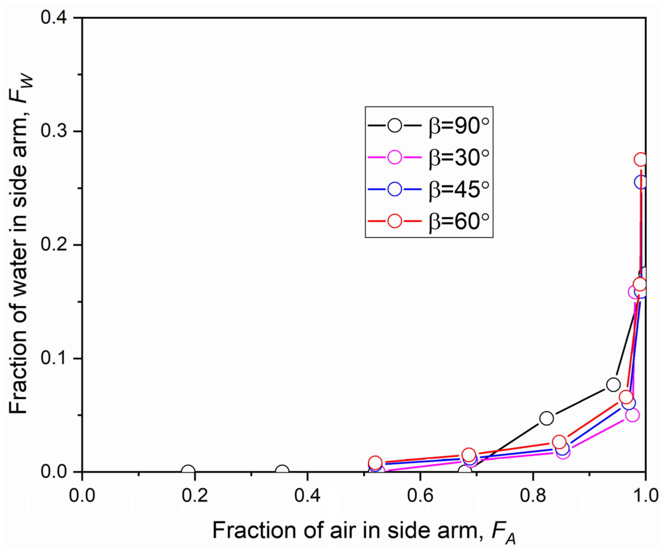
Figure 15 presents $F_A$ versus $F_W$ at different angles of $\beta$. The results show that when $\beta$ is larger, the liquid is only slightly likely to be carried into the side arm at the same air fraction $F_A$. This could be caused by the change in the gas flow direction in the T-shape region leading to a complicated vortex and disturbance streamline, carrying more liquid to the side arm. From this perspective, it is suggested that the inclination angle from the axial direction should be small to avoid liquid entering the side arm. However, Figure 15 also shows that the discrepancies between the results at different $\beta$ are relatively small, so the influence of angle $\beta$ is trivial and can be ignored in the prediction model. Therefore, in order for the mechanical model to be significantly simplified, it is suggested that $\beta$ is fixed.

3. A Prediction Model of the Liquid Carryover Threshold

In this section, a new mechanical model will be proposed to predict the liquid carryover threshold.

3.1. Basic Assumptions

Figure 16 shows the cross section of the T-junction, where the side arm deviates $\mathsf{\alpha }$ from the horizontal plane. To simplify the prediction model, the following assumptions will be used in this work:

• According to the results from Section 2, the inclination angle from the axial direction of the main pipe, $\beta$, has little influence on phase separation, so the effect of $\beta$ can be ignored in the prediction model. For simplification, $\beta$ is fixed at $90°$ in this model.
• Assuming that the gas and liquid two-phase flow in the T-junction reaches the steady state, the concept of separation of the two-phase flow can be used. This concept assumes that the gas and liquid are totally separated and there is a distinct interface between the two phases. Additionally, the entrainment process is ignored. Then, the conservation equation can be developed for gas and liquid, respectively. Considering the goal of this model is to predict the liquid carryover threshold, which is a steady parameter, the assumption that it is at a steady state is reasonable.
• Considering that the flow pattern is stratified, the cross section can be divided into two parts: one is occupied by a gas phase, and another is occupied by a liquid phase. In stratified flow, there is a clear interface between the gas and liquid. This work assumes that the liquid begins to enter the side arm when the water level exceeds $h_s$. Here, $h_s$ represents the distance between the side arm and pipe bottom.
• A gas–liquid interface naturally exists in stratified flow. Generally, the position of the interface can be estimated using the two-phase separated model. However, it should be noted that there are also other forces that affect the water level in the T-junction. As reported in previous works [1,2], the centripetal force in the T-junction is the dominant force sucking the liquid up through the side arm. To take this phenomenon into account, this model assumes that the water level in the T-junction consists of $h_p$ and $h_l$. Here, $h_l$ is the water level calculated using the separated model, and $h_p$ is the water level caused by the sucking effect.

3.2. Establishment of the Prediction Model

With the assumptions listed above, the critical status of the liquid entering the side arm can be expressed by:

$$h_s=h_p+h_l,$$

(1)

Through the geometric analysis, $h_s$ can be calculated using Equation (2), where $D$ is the diameter of the main pipe and $D_s$ is the diameter of the side arm.

$$h_s=\frac{D}{2}\left(1+\sin \alpha \right),$$

(2)

The following subsections will discuss the calculation of $h_p$ and $h_l$.

3.2.1. The Water Level Caused by the Stratified Flow

The water level caused by the stratified flow, $h_l$, can be calculated using the separation model. Figure 17 is a schematic of the stratified gas and liquid flow. The force equilibrium equations for the gas and liquid layers in the axial direction are shown in Equations (3) and (4).

$$-{\tau }_{WG}{S}_g-{\tau }_i{S}_i-A_g\frac{dP}{dL}=0,$$

(3)

$$-{\tau }_{WL}{S}_l+{\tau }_i{S}_i-A_l\frac{dP}{dL}=0,$$

(4)

where ${\tau }_{WG}$ and ${\tau }_{WL}$ are the wall stresses of the gas phase and liquid phase, respectively. ${\tau }_i$ denotes the interfacial stress. $S_g$ and $S_l$ are the perimeters occupied by the gas and liquid phases, respectively. $A_g$ and $A_l$ are the averages of the gas and liquid phases, respectively. $\frac{dP}{dL}$ is the pressure gradient in the axial direction of the main pipe.

Combining Equations (3) and (4), the pressure gradient, $\frac{dP}{dL}$, can be eliminated and Equation (13) can be derived:

$${\tau }_{WG}\frac{S_g}{A_g}-{\tau }_{WL}\frac{S_l}{A_l}+{\tau }_i{S}_i\left(\frac{1}{A_g}+\frac{1}{A_l}\right)=0,$$

(5)

Then, $S_l$, $S_g$, and $S_i$ can be calculated using

$$S_l=D\arccos \left(\frac{\frac{D}{2}-h_l}{\frac{D}{2}}\right),$$

(6)

$$S_g=\pi D-S_l,$$

(7)

$$S_i=D\sin \left[\arccos \left(\frac{\frac{D}{2}-h_l}{\frac{D}{2}}\right)\right],$$

(8)

The wall shear stress and interfacial stress are calculated with

$${\tau }_{WL}=f_L\frac{{\rho }_L{v}_L{}^2}{2},$$

(9)

$${\tau }_{WG}=f_G\frac{{\rho }_G{v}_G{}^2}{2},$$

(10)

$${\tau }_i=f_i\frac{{\rho }_G{\left(v_G-v_i\right)}^2}{2},$$

(11)

Here, $f_L$, $f_G$, and $f_i$ are the friction factors that can be expressed by

$$f_L=C_L{\left(\frac{D_L{v}_L}{{\upsilon }_L}\right)}^{-n},$$

(12)

$$f_G=C_G{\left(\frac{D_G{v}_G}{{\upsilon }_G}\right)}^{-m},$$

(13)

Here, $C_L$, $C_G$, n, and m are constant parameters that depend on the flow status [29,30]. The value used for $C_L=0.046$, $C_G=0.046$, m = 0.2, n = 0.2 for turbulent flow, and $C_L=16$, $C_G=16$, m = 1, n = 1 for laminar flow. $D_L$ and $D_G$ are the hydraulic diameters of the liquid and gas phases, respectively.

$$D_L=\frac{4A_L}{S_L},$$

(14)

$$D_G=\frac{4A_G}{S_G+S_i},$$

(15)

3.2.2. The Water Level Caused by the Sucking Effect

It should be noted that the sucking effect is relatively complex, hence deriving an analytical or numerical relation using physical mechanisms is impractical. Additionally, the entrainment behaviors can occur during the phase separation process. To simplify the mechanical model and consider these complicated flow phenomena, this work will develop a semi-empirical relation based on a physical understanding of the sucking effect and experimental data. From the findings reported from previous works, it can be inferred that the liquid carryout performance is related to the diameter ratio, the gas fraction in the side arm, the gas flow rate, and the phase properties. According to a physical understanding alone, it is clear that with a higher portion of gas in the side, a small diameter ratio, and a larger gas Reynolds number, more liquid can be carried to the side arm. Therefore, it is assumed that $h_p$ is proportional to the fraction of gas in the side arm, $F_A$, and the Reynolds number of the gas phase, $R{e}_g=\frac{{\rho }_g{v}_{G}D}{{\mu }_g}$, and inversely proportional to the diameter ratio, $R_D (\frac{D_s}{D}$). Then, Equation (16) can be used to predict the water level, $h_p$. Here, the parameters of $a$, $b$, $c$, and $d$ are empirical quantities that should be determined according to experimental data.

$$h_p=a{F}_A{}^b{R}_D{}^{c}R{e}_g{}^d,$$

(16)

3.3. Verification of the Proposed Model

To investigate the effect of the diameter ratio on phase separation in the T-junction, Saieed et al. [25] carried out a series of experiments on a specially designed flow loop, whose main pipe was composed of 0.078 diameter PVC pipes. Five diameter ratios were investigated in their work: 0.20, 0.27, 0.52, 0.67, and 1.0, corresponding to the side arm diameters of 0.016 m, 0.021 m, 0.041 m, 0.052 m, and 0.078 m. The side arm was fixed vertically to the horizontal plane, which means $\alpha =90°$ and $\beta =90°$. Three gate valves were used to control the flow rates in the main arm, run arm, and side arm. A camera was adopted to record the phase separation at the T-junction. Nine test cases were used in the experiment with different superficial air and water velocities, as presented in

Table 1. Air and water superficial velocities in the experiments of Saieed et al. [25].

Test Case	Air Superficial Velocity (m/s)	Water Superficial Velocity (m/s)
1	0.178	0.094
2	0.178	0.132
3	0.178	0.176
4	0.228	0.094
5	0.228	0.132
6	0.228	0.176
7	0.288	0.094
8	0.288	0.132
9	0.288	0.176

. In total, 45 liquid carryout threshold data points at various flow velocities and diameter ratios were reported in their work.

Before verification, the constant parameters in Equation (17) should be determined. This work determines these parameters according to the datasets from Saieed et al.’s [25] experiments. Empirically, $a$, $b$, $c$, and $d$ are determined to be $4\times {10}^{-5}$, $5$, $-0.8$, and 1. Then, we have the following:

$$h_p=4\times {10}^{-5}{F}_A{}^5{R}_D{}^{-0.8}R{e}_g,$$

(17)

Figure 18 plots the predicted data versus the experimental data. It can be seen that all of the data points are located close to the diagonal axis, and the relative error is less than 10%. Specifically, the average relative error of the prediction model is 4.16%, which is acceptable for engineering applications. However, it should be noted that because the new model used empirical parameters in Equation (17), the accuracy and application range depend on these empirical relations. In this work, the application range of the new model is at a superficial air velocity from 0.178 m/s to 0.288 m/s, a superficial water velocity from 0.094 m/s to 0.176 m/s, and a diameter ratio from 1.0 to 0.2, and the side arm is fixed to the horizontal plane. To expand the application range of the new model, more experimental data are required; this is expected to be improved upon in the future.

4. Conclusions

In this paper, the effect of the orientation angle of the side arm is investigated using a CFD simulation. The two-phase mixture model is used to simulate the gas and liquid phases in the T-junction, and the reliability of the CFD simulation is verified using the experimental data from published works. Two inclination angles are used to determine the orientation: the deviated angle ($\mathsf{\alpha }$) from the horizontal plane and the deviated angle from the axial direction of the main pipe ($\mathsf{\beta }$). For the deviated angle from the horizontal plane, $\mathsf{\alpha }$, it is found that it is easier for the liquid to be carried to the side arm if $\mathsf{\alpha }$ is small. If $\mathsf{\alpha }$ is small and the water level of the stratified flow is high enough to submerge the side arm, the liquid can enter the side arm directly. So, to avoid liquid carryover, it is suggested that the angle of $\mathsf{\alpha }$ is $90°$, i.e., vertical to the horizontal plane. For the deviated angle from the axial direction of the main arm, $\mathsf{\beta }$, the results show that slightly more liquid can be carried to the side arm when $\mathsf{\beta }$ is close to $90°$. However, overall, the liquid carryover threshold is not sensitive to $\mathsf{\beta }$. So, it is suggested that the inclination angle of $\mathsf{\beta }$ is ignored in the prediction model.

Based on the simulation results and a physical understanding of the phase separation in the T-junction, a new prediction model for the liquid carryover threshold is developed. The effect of $\mathsf{\beta }$ is ignored, so it is fixed to $90°$ in this model. It is assumed that if the water level of the stratified flow in the main arm submerges the side arm, liquid carryover begins. The sucking effect in the T-shape region, which contributes to a higher water level, is also taken into consideration. Experimental datasets from published works are used to validate this model. The results show that the relative error between the measured data and the predicted data is 4.16%, indicating that the new model can accurately predict the liquid carryover threshold. To improve the performance of the new model, more experimental datasets from various operation conditions are required; this is expected to be provided in the future.