
Numerical Investigation on the Flow Instability of Dispersed Bubbly Flow in a Horizontal Contraction Section


Abstract
:1. Introduction
2. Numerical Methodology
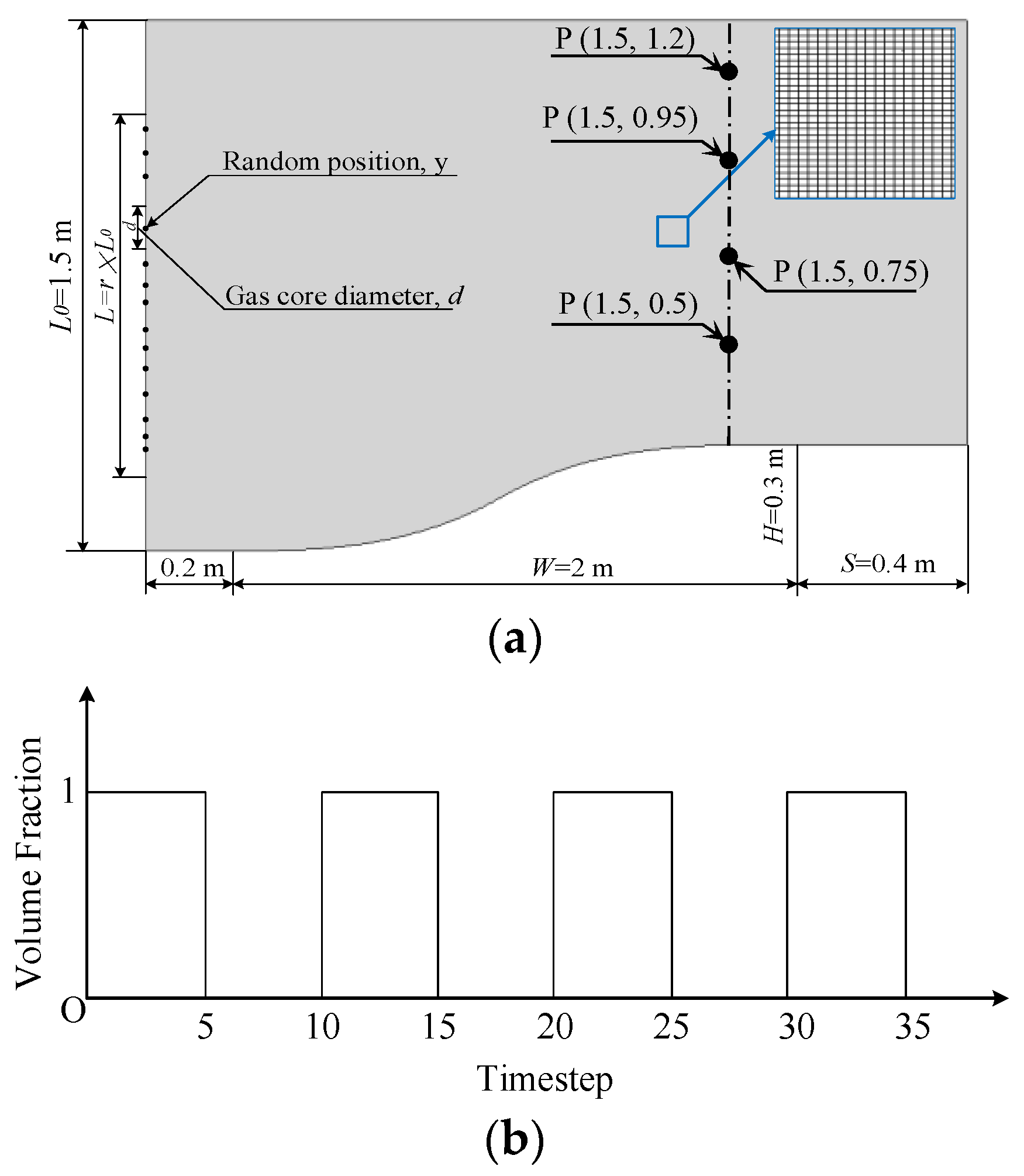
2.1. Computational Conditions
2.2. Governing Equations
2.3. Solution Method
3. Results and Discussion
3.1. Comparison with Experimental Results
3.2. Effect of Bubble Parameters on Flow Instability
3.3. Bubble-Induced Turbulence
3.4. Bulk Void Fraction
4. Conclusions
- (1)
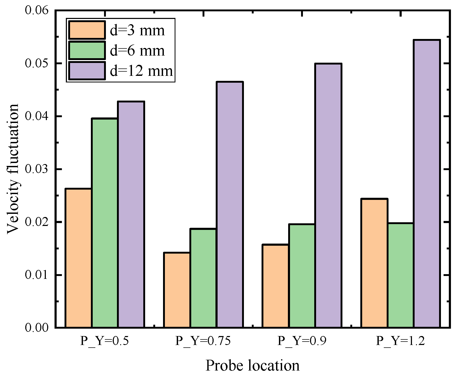
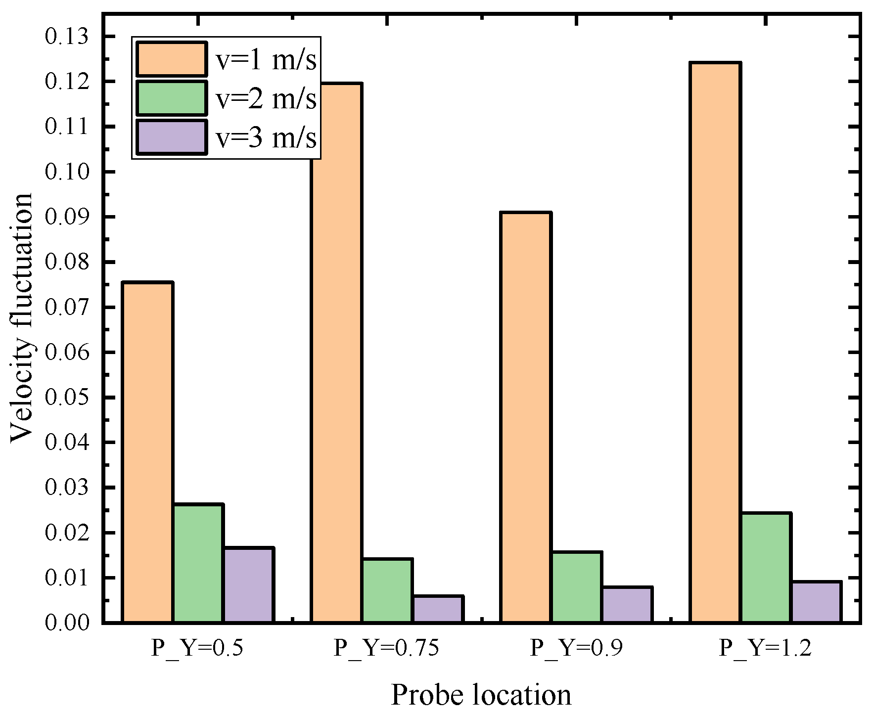
- The presence of bubbles dramatically influences the velocity field and turbulence kinetic energy. The magnitude of velocity fluctuation increases with increasing bubble diameter; this is especially important for low-velocity flow conditions.
- (2)
- For bubble swarm with a concentrated distribution, velocity fluctuation is much higher in the central zone when compared to in the boundary region. However, when considering bubble swarm with sparse distribution, a contrary phenomenon is observed.
- (3)
- Bubble-induced turbulence disturbs the velocity boundary layer near the boundary wall; this will potentially result in enhancing heat and mass transfer by introducing overheating micro-bubbles.
- (4)
- An analysis was performed on dispersed bubbly flow and this is helpful in understanding bubble floatation, which is important in various engineering applications. Foundations in this work can be used as guidance and extended for the design of drag-reduction characteristics of submerged moving objects under dispersed, small/micro, bubbly flow conditions.
Author Contributions
Funding
Institutional Review Board Statement
Informed Consent Statement
Data Availability Statement
Acknowledgments
Conflicts of Interest
Nomenclature
| Cd | drag coefficient |
| DIV | number of bubble cores |
| d | gas core diameter, m |
| g | gravity acceleration, m s−2 |
| k | turbulence kinetic energy, m2 s−2 |
| L0 | length scale of inlet, m |
| L | length scale of bubble region, m |
| p | pressure, Pa |
| Pr | Prandtl number |
| r | region factor, r = L/L0 |
| Re | Reynolds number |
| T | temperature, K |
| t | Solution time, s |
| v | averaged velocity, m s−1 |
| vg | gas phase velocity, m s−1 |
| Greek symbols | |
| αg | volume fraction of gas phase |
| αw | volume fraction of water phase |
| μ | viscosity, Pa s |
| μt | turbulent viscosity, Pa s |
| ρ | mean density, kg m−3 |
| ω | specific dissipation rate |
| κ | curvature, m−1 |
| ∇ | partial differential operator |
| Γ | effective diffusivity |
| Subscripts | |
| csf | continuum surface force model |
| drag | drag force |
| w | water phase |
| g | gas phase |
References
- Tahir, W.; Althobaiti, N.; Kousar, N.; Alhazmi, S.E.; Bilal, S.; Riaz, A. Effects of Homogeneous-Heterogeneous Reactions on Maxwell Ferrofluid in the Presence of Magnetic Dipole Along a Stretching Surface: A Numerical Approach. Math. Probl. Eng. 2022, 8, 4148401. [Google Scholar] [CrossRef]
- Chen, P.; Cui, B.; Li, J.; Zheng, J.; Zhao, Y. Particle Erosion under Multiphase Bubble Flow in Horizontal-Vertical-Upward Elbows. Powder Technol. 2022, 397, 117002. [Google Scholar] [CrossRef]
- Iqbal, M.S.; Malik, F.; Khan, L.; Ghaffari, A.; Riaz, A.; Nisar, K. Sooppy Impact of Induced Magnetic Field on Thermal Enhancement in Gravity Driven Fe3O4 Ferrofluid Flow through Vertical Non-Isothermal Surface. Results Phys. 2020, 19, 103472. [Google Scholar] [CrossRef]
- Ijaz, N.; Riaz, A.; Zeeshan, A.; Ellahi, R.; Sait, S.M. Buoyancy Driven Flow with Gas-Liquid Coatings of Peristaltic Bubbly Flow in Elastic Walls. Coatings 2020, 10, 115. [Google Scholar] [CrossRef] [Green Version]
- Cheng, F.; Ji, W.; Qian, C.; Xu, J. Cavitation bubbles dynamics and cavitation erosion in water jet. Results Phys. 2018, 9, 1585–1593. [Google Scholar] [CrossRef]
- Oliveira, W.D.; Paula, I.D.; Martins, F.; Farias, P.; Azevedo, L. Bubble characterization in horizontal air–water intermittent flow. Int. J. Multiph. Flow 2015, 69, 18–30. [Google Scholar] [CrossRef]
- Orvalho, S.; Ruzicka, M.C.; Olivieri, G.; Marzocchella, A. Bubble coalescence: Effect of bubble approach velocity and liquid viscosity. Chem. Eng. Sci. 2015, 134, 205–216. [Google Scholar] [CrossRef]
- Sohn, S.; Baek, S. Bubble merger and scaling law of the Rayleigh–Taylor instability with surface tension. Phys. Lett. A 2017, 16, 3812–3817. [Google Scholar] [CrossRef]
- Sanada, T.; Sugihara, K.; Shirota, M.; Watanabe, M. Motion and drag of a single bubble in super-purified water. Fluid Dyn. Res. 2008, 40, 534–545. [Google Scholar] [CrossRef]
- Pang, M.; Wei, J.; Bo, Y.; Kawaguchi, Y. Numerical Investigation on Turbulence and Bubbles Distribution in Bubbly Flow under Normal Gravity and Microgravity Conditions. Microgravity Sci. Technol. 2010, 22, 283–294. [Google Scholar] [CrossRef]
- Chen, T.; Mu, Z.; Huang, B.; Zhang, M.; Wang, G. Dynamic Instability Analysis of Cavitating Flow with Liquid Nitrogen in a Converging–Diverging Nozzle. Appl. Therm. Eng. 2021, 192, 116870. [Google Scholar] [CrossRef]
- Li, G.B.; Wang, Y.R.; Xiao, L.M. Instability of an annular liquid sheet exposed to compressible gas flows. Int. J. Multiph. Flow 2019, 119, 72–83. [Google Scholar] [CrossRef]
- Yang, M.; Lian, C.Y.; Fan, L.S.; Lee, D.J. On the second-order moment turbulence model for simulating a bubble column. Chem. Eng. Sci. 2002, 57, 3269–3281. [Google Scholar]
- Zhou, L.; Li, R.; Du, R. Numerical simulation of the effect of void fraction and inlet velocity on two-phase turbulence in bubble-liquid flows. Acta Mech. Sin. 2006, 22, 425–432. [Google Scholar] [CrossRef]
- Li, W. Two-phase heat transfer correlations in three-dimensional hierarchical tube. Int. J. Heat Mass Transf. 2022, 191, 122827. [Google Scholar] [CrossRef]
- Kawahara, A.; Sadatomi, M.; Nei, K.; Matsuo, H. Experimental study on bubble velocity, void fraction and pressure drop for gas—Liquid two-phase flow in a circular microchannel. Int. J. Heat Fluid Flow 2009, 30, 831–841. [Google Scholar] [CrossRef]
- Peters, F.; Els, C. An experimental study on slow and fast bubbles in tap water. Chem. Eng. Sci. 2012, 82, 194–199. [Google Scholar] [CrossRef]
- Ji, H.; Chang, Y.; Huang, Z.; Wang, B.; Li, H. A new contactless impedance sensor for void fraction measurement of gas—Liquid two-phase flow. Meas. Sci. Technol. 2016, 27, 124001. [Google Scholar] [CrossRef]
- Zhou, X.; Sun, X.; Liu, Y. Liquid-phase turbulence measurements in air-water two-phase flows over a wide range of void fractions. Nucl. Eng. Des. 2016, 310, 534–543. [Google Scholar] [CrossRef]
- Rivera, Y.; Muoz-Cobo, J.L.; Cuadros, J.L.; Berna, C.; Escrivá, A. Experimental study of the effects produced by the changes of the liquid and gas superficial velocities and the surface tension on the interfacial waves and the film thickness in annular concurrent upward vertical flows. Exp. Therm. Fluid Sci. 2021, 120, 110224. [Google Scholar] [CrossRef]
- Wang, J.; Li, Y.; Wang, L.; Mao, H.; Ma, Y.; Xie, F. Experimental investigation on two-phase flow instabilities in long-distance transportation of liquid oxygen. Cryogenics 2019, 102, 56–64. [Google Scholar] [CrossRef]
- Domnick, J.; Durst, F. Measurement of bubble size, velocity and concentration in flashing flow behind a sudden constriction. Int. J. Multiph. Flow 1995, 21, 1047–1062. [Google Scholar] [CrossRef]
- Al-Yahia, O.S.; Yoon, H.J.; Jo, D. Experimental study of bubble flow behavior during flow instability under uniform and non-uniform transverse heat distribution. Nucl. Eng. Technol. 2020, 52, 2771–2788. [Google Scholar] [CrossRef]
- Sokolichin, A.; Eigenberger, G. Applicability of the standard κ-ε turbulence model to the dynamic simulation of bubble columns: Part I. Detailed numerical simulations. Chem. Eng. Sci. 1999, 54, 2273–2284. [Google Scholar] [CrossRef]
- Xgab, C.; Ning, Y. CFD simulation of bubble column hydrodynamics with a novel drag model based on EMMS approach—ScienceDirect. Chem. Eng. Sci. 2021, 243, 116758. [Google Scholar]
- Feng, J.; Bolotnov, I.A. Evaluation of bubble-induced turbulence using direct numerical simulation. Int. J. Multiph. Flow 2017, 93, 92–107. [Google Scholar] [CrossRef] [Green Version]
- Yang, M.; Pozo, D.; Torfs, E.; Rehman, U.; Nopens, I. Numerical simulation on the effects of bubble size and internal structure on flow behavior in a DAF tank: A comparative study of CFD and CFD-PBM approach. Chem. Eng. J. Adv. 2021, 7, 100131. [Google Scholar] [CrossRef]
- Kawamura, T.; Kodama, Y. Numerical simulation method to resolve interactions between bubbles and turbulence. Int. J. Heat Fluid Flow 2002, 23, 627–638. [Google Scholar] [CrossRef]
- Chahine, G.L. Numerical simulation of bubble flow interactions. J. Hydrodyn. Ser. B 2009, 21, 316–332. [Google Scholar] [CrossRef]
- Yi, T.; Chu, X.; Wang, B.; Wu, J.; Yang, G. Numerical simulation of single bubble evolution in low gravity with fluctuation. Int. Commun. Heat Mass Transf. 2022, 130, 105828. [Google Scholar] [CrossRef]
- Bahreini, M.; Derakhshandeh, J.F.; Ramiar, A.; Dabirian, E. Numerical study on multiple bubbles condensation in subcooled boiling flow based on CLSVOF method—ScienceDirect. Int. J. Therm. Sci. 2021, 170, 107121. [Google Scholar] [CrossRef]
- Laborde-Boutet, C.; Larachi, F.; Dromard, N.; Delsart, O.; Schweich, D. CFD simulation of bubble column flows: Investigations on turbulence models in RANS approach. Chem. Eng. Sci. 2009, 64, 4399–4413. [Google Scholar] [CrossRef]
- Brackbill, J.U.; Kothe, D.B.; Zemach, C. A continuum method for modeling surface tension. J. Comput. Phys. 1992, 100, 335–354. [Google Scholar] [CrossRef]
- Ishii, M.; Zuber, N. Drag coefficient and relative velocity in bubbly, droplet or particulate flows. AIChE J. 2010, 25, 638–651. [Google Scholar] [CrossRef]
- Erdogan, S.; Schulenberg, T.; Deutschmann, O.; Wörner, M. Evaluation of models for bubble-induced turbulence by DNS and utilization in two-fluid model computations of an industrial pilot-scale bubble column. Chem. Eng. Res. Des. 2021, 175, 283–295. [Google Scholar] [CrossRef]
- Shu, S.; Bahraoui, N.E.; Bertrand, F.; Chaouki, J. A bubble-induced turbulence model for gas-liquid bubbly flows in airlift columns, pipes and bubble columns. Chem. Eng. Sci. 2020, 6, 227–238. [Google Scholar] [CrossRef]


| Inlet Velocity v, m s−1 | Region Factor, r | Bubble Density. 1, DIV/L0, m−1 | Gas-Core dia. 2 d, mm | Bubble dia. mm | Bulk Void Fraction α% | Reynolds Number | |
|---|---|---|---|---|---|---|---|
| Case 1 | 2.0 | 0.8 | 10/1.2 | 6.0 | 3.91 | 0.358 | 3.5 × 10⁶ |
| Case 2 | 2.0 | 0.8 | 20/1.2 | 6.0 | 3.91 | 0.341 | 3.5 × 10⁶ |
| Case 3 | 2.0 | 0.8 | 20/1.2 | 12.0 | 5.53 | 0.724 | 3.5 × 10⁶ |
| Case 4 | 2.0 | 0.8 | 20/1.2 | 3.0 | 2.76 | 0.341 | 3.5 × 10⁶ |
| Case 5 | 2.0 | 0.8 | 40/1.2 | 6.0 | 3.91 | 0.291 | 3.5 × 10⁶ |
| Case 6 | 1.0 | 0.8 | 20/1.2 | 6.0 | 2.76 | 0.323 | 1.75 × 10⁶ |
| Case 7 | 3.0 | 0.8 | 20/1.2 | 6.0 | 4.79 | 0.352 | 5.25 × 10⁶ |
| Case 8 | 2.0 | 0.6 | 20/0.9 | 6.0 | 3.91 | 0.345 | 3.5 × 10⁶ |
| Case 9 | 2.0 | 0.4 | 20/0.6 | 6.0 | 3.91 | 0.354 | 3.5 × 10⁶ |
| Case 1, v0 = 2 m s−1, DIV = 10, dia. = 6 mm, r = 0.8 | Case 3, v0 = 2 m s−1, DIV = 20, dia. = 12 mm, r = 0.8 | Case9, v0 = 2 m s−1, DIV = 20, dia. = 6 mm, r = 0.4 | |
|---|---|---|---|
| Flow time = 100 ms |  | 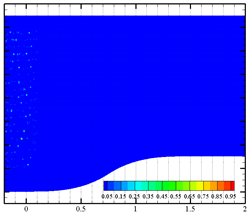 |  |
| Flow time = 400 ms | 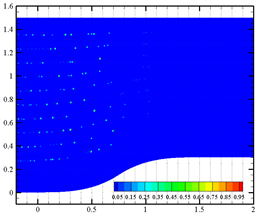 |  |  |
| Flow time = 1000 ms |  |  |  |
| Flow time = 3000 ms |  |  |  |
Publisher’s Note: MDPI stays neutral with regard to jurisdictional claims in published maps and institutional affiliations. |
© 2022 by the authors. Licensee MDPI, Basel, Switzerland. This article is an open access article distributed under the terms and conditions of the Creative Commons Attribution (CC BY) license (https://creativecommons.org/licenses/by/4.0/).
Share and Cite
Chen, J.; Li, W.; Fu, C.; Zhang, J.; Kukulka, D.J. Numerical Investigation on the Flow Instability of Dispersed Bubbly Flow in a Horizontal Contraction Section. Processes 2022, 10, 1389. https://doi.org/10.3390/pr10071389
Chen J, Li W, Fu C, Zhang J, Kukulka DJ. Numerical Investigation on the Flow Instability of Dispersed Bubbly Flow in a Horizontal Contraction Section. Processes. 2022; 10(7):1389. https://doi.org/10.3390/pr10071389
Chicago/Turabian StyleChen, Jingxiang, Wei Li, Cheng Fu, Jingzhi Zhang, and David J. Kukulka. 2022. "Numerical Investigation on the Flow Instability of Dispersed Bubbly Flow in a Horizontal Contraction Section" Processes 10, no. 7: 1389. https://doi.org/10.3390/pr10071389
APA StyleChen, J., Li, W., Fu, C., Zhang, J., & Kukulka, D. J. (2022). Numerical Investigation on the Flow Instability of Dispersed Bubbly Flow in a Horizontal Contraction Section. Processes, 10(7), 1389. https://doi.org/10.3390/pr10071389