Active and Passive Defense Strategies of Cyber-Physical Power System against Cyber Attacks Considering Node Vulnerability

Abstract

Vulnerable parts in the cyber-physical power system can be maliciously attacked to trigger cascading failures. This paper proposes a defense framework with active and passive defense hybrid strategies. First, a comprehensive vulnerability assessment index is presented to identify vital nodes contributing to failure extension. The proposed index is based on both physical characteristics and topology. Physical characteristic is assessed through the optimal power flow to calculate the load losses. The topology index is obtained by the attacking node and calculating the nodes lost at the steady state. Then, the active and passive defense strategies are established. Deploying false nodes based on the comprehensive vulnerability index is set as the active defense strategy. Changing from centralized control mode to centralized-distributed control mode is the passive defense strategy. The system can defend against attacks with active and passive strategies effectively in the attacking experiments. Finally, we have made a profound study of the first-order percolation problem. The first-order percolation disappears under the active and passive defense strategies in a scale-free network, while the small world network transfers from the first-order percolation to the second-order percolation. The findings indicated that the diverse results resulted from their structure.

1. Introduction

Power grid is a large interconnected system whose reliable operation depends critically on its cyber infrastructure [1]. It is gradually developing into a cyber-physical power system (CPPS). The close and complex interdependences between the cyber network and physical network are one of the major characteristics of CPPS. The cyber network provides strong support of the precise control for power grid while a failure in the cyber network may be expanded to the physical network, which can trigger a breakout in the power grid [2]. Ukraine grid blackout caused by hostile attack resulted in knocking out the lights for 250,000 people in 2015. It is a great challenge to identify vulnerabilities and defend against numerous attacks effectively, especially getting ready for potential attacks.

1.1. Vulnerability Assessment

To facilitate understanding of the security risks, numerical studies have been carried out on vulnerability assessment. Current research mainly analyzes two perspectives: physical properties and system structure. However, studies considering only physical properties or system structure have limitations. It can not provide an accurate and practical index for system operators. It is not clear how serious of an impact has been made on the system.

Ref. [3] proposed a vulnerability assessment method for deep reinforcement learning models in power systems topology optimization under cyber attack. Attack centrality metric based on both the damage and cost of a component attack is proposed to provide greedy hybrid attack algorithms and optimal hybrid attack algorithms [4]. The performance of these algorithms has been validated through the experiments on IEEE bus data. Quantitative factors affecting resiliency and utilizing concepts are integrated into a single metric using a multi-criteria decision making (MCDM) technique to solve the assessment problem [5]. A vulnerability assessment method for the coupled network is proposed. It takes both power and electric vehicle energy network properties into consideration with a hybrid power transfer distribution factor [6]. The random matrix model is applied into the critical bus identification problem. The data-driven method proposed can solve the problems of vulnerability assessment of complex power systems without modeling. It has better accuracy than previous methods [7]. A new concept of Hybrid Attack Graph (HAG) is introduced to capture the evolution of both logical and real values of system parameters [8]. The vulnerability of the grid was analyzed using the machine learning and game theory from the attacker’s viewpoints [9]. All researches above only concentrate on one aspect of the grid or cyber network, and very few have considered the influence brought by both networks or put up a comprehensive index from two perspectives. Factors affecting cyber-physical resiliency of transmission systems are outlined and computed based on both physical and cyber aspects [10]. However, it still has limitations in that it separates CPS into two independent networks ignoring their mutual connection.

Some complex network theories are used to analyze vulnerability parts of CPPS. The interdependent power network disruptor (IPND) is proven as an NP-hard problem. A new evaluation index is proposed to measure the impacts on the network under sequential attacks [11]. The power grid coupled with double-star networks has a lower probability of failure than the mesh structure. Whereas, the method neglected the physical characteristics and simplified the issue into topology structure. There is still controversy over whether the first-order percolation or second-order percolation exists. Once the first-order percolation exists, the consequences can be catastrophic. The system can be paralyzed and all nodes are out of control. Osman Yagan insists that there is first-order percolation with the increasing number of attacking nodes [12]. There is a threshold for the proportion of faulty nodes, which leads to the second-order percolation [13]. The first-order percolation may not happen in the real grid based on the true data from five provinces and one city of China [14].

There remains a major challenge of detecting the most vulnerable parts in the CPPS taking physical characteristics and system structure into consideration.

1.2. Defense Strategy

The main challenge faced by researchers is defending various attacks and controlling properly. Most of the existing defense strategies can be divided into two categories, active defense and passive defense.

Active defense is a prevention mechanism before malicious attacks. The strategy will be carried out by employing redundant resources and enhancing the security level when the threat does not occur or cause serious consequences. Honeypots are introduced into the advanced metering infrastructure as a decoy to detect and gather attack information [15]. The evolving defense mechanism (EDM) based on a bio-inspired idea of network configuration variations avoids the deficiency of conventional mechanisms and has the potential to cope with emerging security threats [16]. Ref. [17] reached beyond the traditional one-sided security defense systems and proposes the concept of cyber-physical coordinated situation awareness and active defense to improve the ability of CPPS. Such active defense strategies, however, have failed to address the destroying situation. It is not enough to defend against increasingly complicated attacks by only relying on an active defense strategy.

Passive defense refers to taking advantage of system characteristics to correct the damaged data and control signals after attacking. A tractable cyber-enabled adaptive control scheme based on feedback linearization control is effective to address attacks on data integrity and availability [18]. A model for the competition between the cascading failures and restoration strategy is developed to repair failed nodes into the boundary of the functional network [19]. A strategy of reconnecting every isolated component to the giant component is an effective method to avoid collapsing [20]. Such approaches, however, have failed to address how to correct and control failed nodes in detail.

Active and passive defense strategies should be combined. Similarly, it is paramount to detect and predict potential faults and implement resilient control to avoid dangerous situations for wind turbine systems. Prognosis can be regarded as an active defense mechanism and resilient control is a passive method [21].

The goal of this paper is to set up a comprehensive index to assess CPPS vulnerability. Both physical characteristic and topology should be taken into account. Active and passive hybrid defense strategies are established combining false nodes according to the index and distributed control nodes.

As far as we know, our work is the first to adopt active and passive defense strategies in detail. The strategies combine false nodes and distributed control nodes to correct and control nodes. The main contributions are summarized as follows:

(1) An efficient vulnerability assessment analysis is proposed by the comprehensive vulnerability index. The index is derived from physical characteristics and system structure. It makes up for the deficiency of considering only from a single aspect.

(2) Active and passive hybrid defense strategies are established to defend the adversarial attacks. False nodes as decoys are deployed to mislead attackers based on the vulnerability analysis. Distributed control nodes are applied from the centralized control mode to the centralized–distributed control mode. Compared to the adding edges method, active and passive defense strategies are comparably more effective and the defense effect is more obvious.

(3) The robustness of CPPS can be improved to a great extent. The simulations suggest that the scale-free network can avoid percolation with the active and passive defense strategies while small world network transfers from the first-order percolation to the second-order percolation. This difference can be explained with their structure. The defense effect is more obvious in the scale-free network than the small world network. The difference can be instructive to the construction of communication network.

The rest of the paper is organized as follows. Section 2 presents the vulnerability analysis. In Section 3, active and passive defense strategies are developed. Case study and discussion are shown in Section 4, and conclusions are drawn in Section 4.

2. Vulnerability Analysis

Based on the cyber-physical power system model, vulnerable nodes are identified by the comprehensive vulnerability index from physical characteristics and system structure. The physical characteristics index is expressed with load shedding while system structure index is analyzed with the node lost. The critic weight method is adopted to identify the weight of two indexes to get the comprehensive vulnerability index.

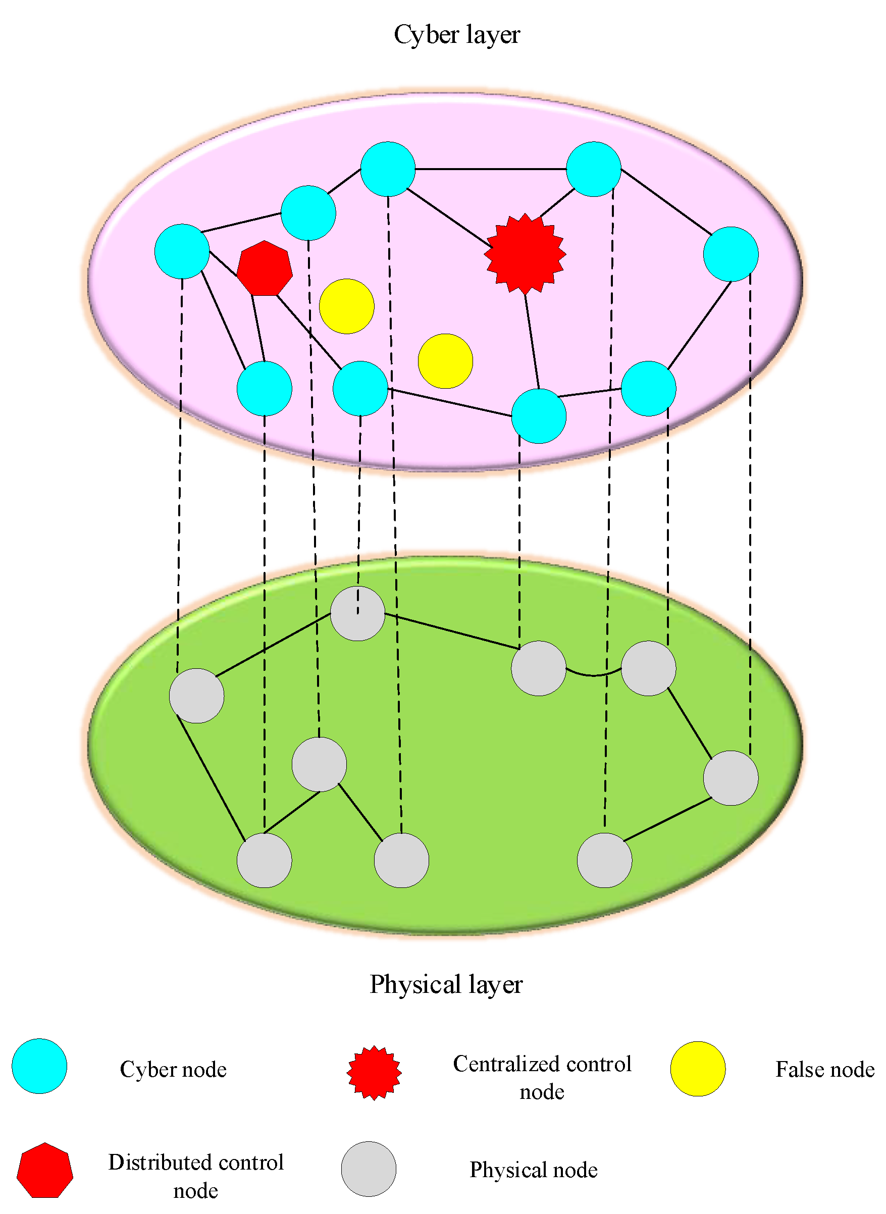
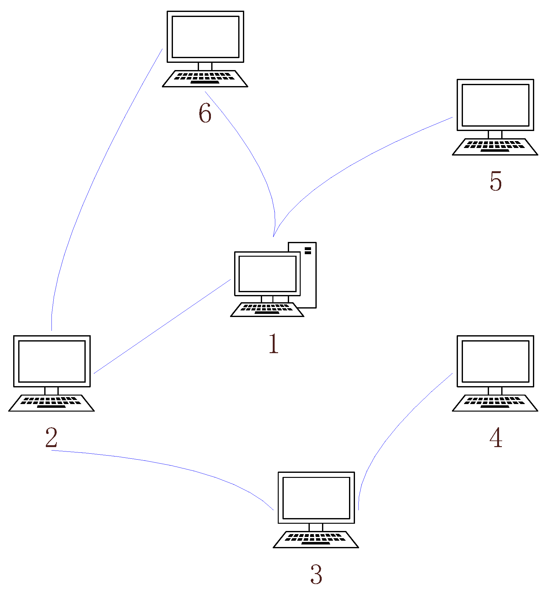
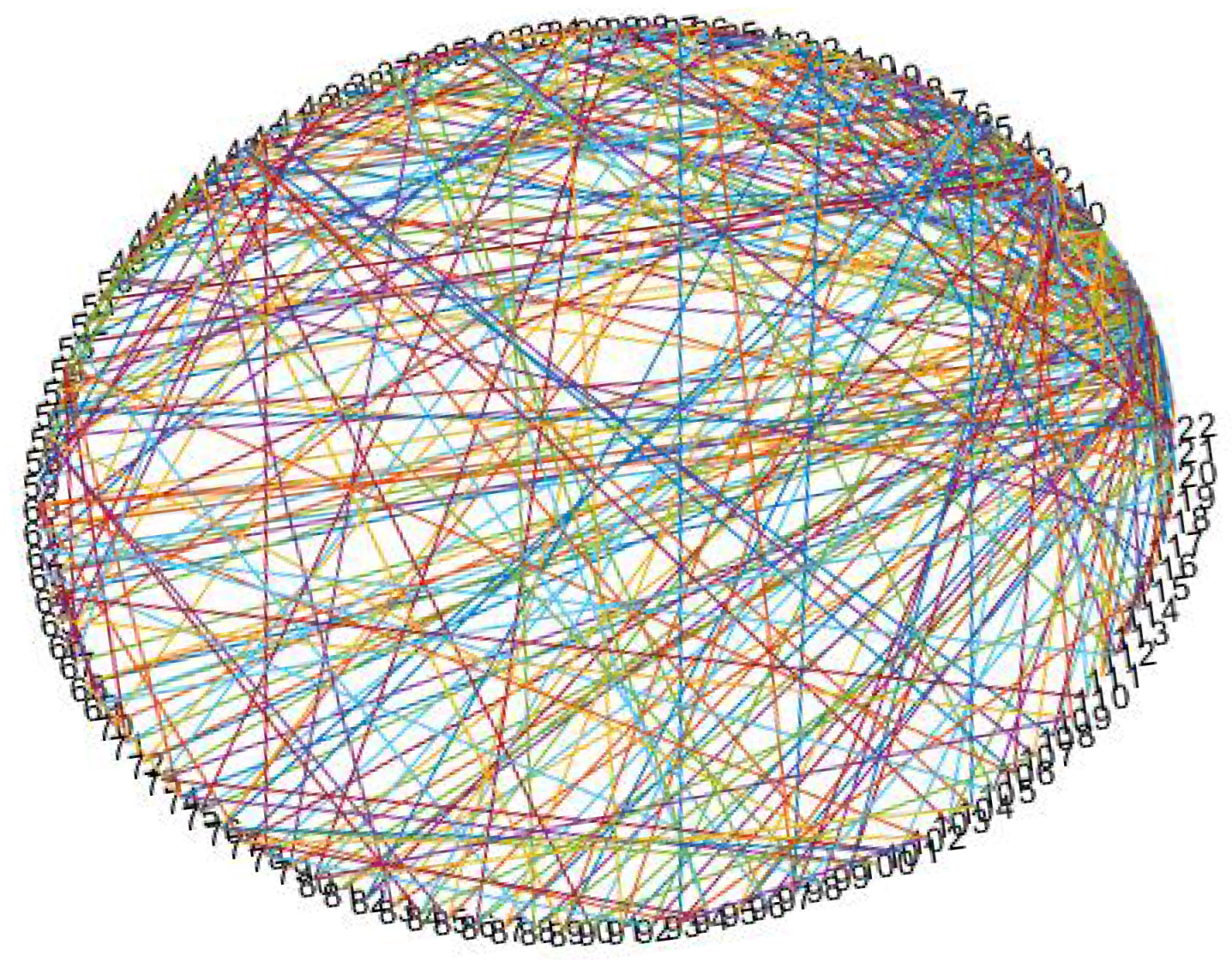
2.1. Cyber Physical System Model

Cyber-physical power system (CPPS) consists of the physical layer and the cyber layer, which is seen as an interconnected network. The schematic diagram of CPPS is shown in Figure 1.

CPPS is modeled as a complex network. It describes the interactions and connectivity between the physical layer and the cyber layer. The physical layer and cyber layer can be considered as a large complex network with nodes and edges, separately. Physical nodes in the power grid supply electricity for cyber nodes while cyber nodes monitor, measure, and control physical nodes and vice versa. However, some important cyber nodes such as centralized control nodes have independent power supply and are not entirely dependent on physical nodes. Such nodes are called independent nodes. Degree and betweenness are two major metrics representing static characteristics in complex networks. The interdependency between the physical layer and the cyber layer generally means that the normal operation of one node in the network depends on the corresponding nodes in the other network. The interdependency may lead to cascading failure and cause a breakout in the power grid. However, the system becomes extremely robust when adopting the interdependency of ‘degree to betweenness’ [22], i.e., the node with the largest degree in the cyber layer is coupled with the node with the largest betweenness in the physical layer. The interdependency of ‘degree to betweenness’ is adopted in our work to test the roubustness of the system. The adjacency matrix A and B are to define the connectivity of the physical graph and cyber graph, separately.

$$\begin{array}{cc}\hfill & A(i,j)=\left\{\begin{array}{cc}1\hfill & \mathrm{there}\mathrm{is}\mathrm{a}\mathrm{connection}\mathrm{between}\mathrm{node}i\mathrm{and}\mathrm{node}j\hfill \\ 0\hfill & \mathrm{there}\mathrm{is}\mathrm{no}\mathrm{connection}\mathrm{between}\mathrm{node}i\mathrm{and}\mathrm{node}j\hfill \end{array}\right.\hfill \end{array}$$

(1a)

$$\begin{array}{cc}\hfill & B(i,j)=\left\{\begin{array}{cc}1\hfill & \mathrm{there}\mathrm{is}\mathrm{a}\mathrm{connection}\mathrm{between}\mathrm{node}i\mathrm{and}\mathrm{node}j\hfill \\ 0\hfill & \mathrm{there}\mathrm{is}\mathrm{no}\mathrm{connection}\mathrm{between}\mathrm{node}i\mathrm{and}\mathrm{node}j\hfill \end{array}\right.\hfill \end{array}$$

(1b)

According to Equation (1), matrix B of the network in Figure 2 is $B=\left|\begin{array}{c}010011\hfill \\ 101001\hfill \\ 010100\hfill \\ 001000\hfill \\ 100000\hfill \\ 110000\hfill \end{array}\right|$.

Graphs with complex network theory are mainly concerned with the statistical properties with nodes and edges. Some vital metrics used later are listed as follows:

•

Degree distribution

The degree distribution of nodes in the network can be described by a distribution function P(k), which presents the proportion of the nodes with k degrees in all nodes in the network. That is, the probability of k degree nodes is P(k) when selecting a node randomly.

$$\begin{array}{cc}\hfill P\left(k\right)& =\frac{N_k}{M}\hfill \end{array}$$

(2)

where,

$N_k$ is the number of nodes with the degree k in the network;

M is the total number of nodes in the network.

•

Clustering coefficient

Similar nodes have the characteristic of clustering together, which is called the clustering property of networks in complex theory. The property is represented by the clustering coefficient (CLU).

$$\begin{array}{c}\hfill CL{U}_i=\frac{E_i}{{clu}_{ki}^2}\end{array}$$

(3)

where,

$E_i$ is the number of edges that actually exist between the node $k_i$ and its adjacent nodes;

${clu}_{ki}^2$ is the total number of possible edges around the node $k_i$.

Specifically, the clustering coefficient in the small world network can be formatted as in (4).

$$CL{U}_{sw}=\frac{3(k-2)}{4(k-1)+4kp(p+2)}$$

(4)

where,

k is the number of nodes connected to each node from the regular network when constructing the small world network;

p is the probability of adding an edge between two nodes selected randomly.

In a scale-free network, the clustering coefficient can be calculated as (5).

$$CL{U}_{Sf}=\frac{m^2{\left(m+1\right)}^2}{4(m-1)}\left[\mathrm{In}(\frac{m+1}{m})-\frac{1}{m+1}\right]\frac{{\left[\mathrm{In}\left(T\right)\right]}^2}{T}$$

(5)

where,

m is the number of connections to existing nodes when a new node is generated to construct the network;

T is the final number of new nodes.

•

Modular Q

Q describes the modular level of the community quantitatively. We define a symmetric matrix $E= ({\mathrm{e}}_{ij}{)}_{c\times c}$. The element $e_{ij}$ in E is the proportion of edges connecting nodes of two communities i and j in all edges.

$$Q=\sum _{i=1}^c(e_{ii}-{b_i}^2)=t-\left|\right|E^2\left|\right|$$

(6)

where,

$$b_i={\sum }_{j=1}^c{e}_{ij}$$

(7)

$$t={\sum }_{i=1}^c{e}_{ij}$$

$\left|\right|E^2\left|\right|$ is sum of elements in $E^2$.

2.2. Phisical Characteristic Index

Load shedding index (LSI) is an important index to analyze the changing nature of the load and its effect on grid vulnerability. The optimal power flow (OPF) is widely used to analyze the load shedding. To recognize and assess the vulnerability of nodes, every node in the power grid is attacked and the LS of the node is formulated as (8):

$$\begin{array}{c}minLS{}_k=\sum _{i=1}^n\Delta P_{Fi}\end{array}$$

(8a)

$$\begin{array}{c}\mathrm{s}.\mathrm{t}F=A_{F-P}P\end{array}$$

(8b)

$$\begin{array}{c}\sum _{i=1}^n\left(P_{Gi}+\Delta P_{Gi}-\left(P_{Fi}-\Delta P_{Fi}\right)\right)=0\end{array}$$

(8c)

$$\begin{array}{c}\left|F_l\right|\le F_{lmax}\end{array}$$

(8d)

$$\begin{array}{c}0\le \Delta P_{Fl}\le P_{Fl}\end{array}$$

(8e)

where $L{s}_k$ is the total load shedding when attacking the node k; $\Delta P_{Fi}$ is the load reduction at node i; n is the number of nodes in the power grid; F is the branch flow; $A_{F-P}$ denotes the admittance matrix; P calculates the power flows to the node; $P_{Gi}$ are the outputs of the generator; $\Delta P_{Gi}$ is generator output adjustment; $P_{Fi}$ are loads of the node i; $|F_l|$ indicates the flow of branch l; $F_{lmax}$ are the limits of branch l.

The load shedding (LS) is calculated by OPF. The major steps can be expressed as follows:

Step 1 (Initialization): Get information on the loads and generators and calculate the power flows;

Step 2 (Attacking): Attack node in the power grid in turn; remove the branches linking to the node attacked;

Step 3 (Load Redistribution): Based on OPF, adjust generators and loads;

Step 4 (Calculating): Calculate the total load shedding as (8).

2.3. Topology Structure Index

In the dynamics of cascading failures, the robustness of different communication networks are tested by computing the number of nodes survived at the end of attacking. It is assumed that a node is functioning if it satisfies the percolation theory.

(1) The node has the interlinks from the other network, i.e., its corresponding node can survive.

(2) The node belongs to the giant connected component of its network.

It is assumed that the cascading failure is triggered by a fraction of the nodes in the cyber network, i.e., a fraction of the nodes are attacked. Attacking is simulated by removing a fraction of the nodes in the cyber network. Once a node is removed, its edges in the cyber network and inter edges in the physical network are deleted. Only the nodes in the giant connected component of the cyber network can operate properly due to condition 2. That will lead to more nodes and edges being removed. Owing to the interdependence, some nodes in the physical network may dysfunction since they lose their inter edges. The physical network may fragment into components. In such a situation, the working nodes are those belonging to the giant connected component of the physical network. As more and more nodes and edges are removed, the fragmentation in the physical network may result in further failures in the cyber network. Continuing in this manner, the failures propagate alternately between the cyber network and the physical network, reaching one of the following states: (1) system collapses, (2) residual giant connected components in both networks. For convenience, the notations used in the cascading failures are summarized in

Table 1. Key notations in the analysis of cascading failures.

$P_0$, $C_0$	The initial condition of physical network and cyber network (not suffering attacks)
M, N	The scale of physical network and cyber network
$P_k$, $C_k$	The giant connected components in $P_k^{\prime }$ and $C_k^{\prime }$ (the survival nodes at stage i + 1)
$P_k{}^{\prime }$, $C_k{}^{\prime }$	The sets of remaining nodes in $P_k^{\prime }$ and $C_k^{\prime }$ which have supporting interlinks at stage i
${\mu }_{p_i}$, ${\mu }_{c_i}$	The fractions corresponding to retaining the interlink $P_{k^{\prime }}={\mu }_{p_i}{P}_k$, $C_k^{\prime }={\mu }_{c_i}{C}_k$
${\mu }_{p_i}^{\prime }$, ${\mu }_{c_i}^{\prime }$	The fractions corresponding to giant connected components $P_{k+1}={\mu }_{p_i}^{\prime }{P}_k^{\prime }$, $C_{k+1}={\mu }_{c_i}^{\prime }{C}_k$
F(X) components by the matrix X	The function of solving the giant connected

.

Stage 1: Failure of nodes in the cyber network

It is assumed that the cyber network is normal at first. $A_{}(i,j)$ and $B_{}(i,j)$ are derived based on links between nodes in networks. Numerous attacks are simulated with removal of a fraction $1-\varphi$ of nodes in C. As a result, $A_{}(i,j)$ is devised accordingly, e.g., if the node i is attacked, the elements in the row i and the column i are modified to be zero. The remaining network $C_0{}^{\prime }$ has size ${\mu }_{c_0}N$. In this stage, $C_0{}^{\prime }$ may fragment into clusters. Since only the nodes contained in the giant connected component are at work, the giant component $C_1$ can be calculated by $F\left(A\right)$.

$$C_1={\mu }_{c_0}{}^{\prime }{C}_0^{\prime }={\mu }_{c_0}{\mu }_{c_0}{}^{\prime }{C}_0={\mu }_{c_0}{\mu }_{c_0}{}^{\prime }N$$

(9)

It is necessary to determine the size of the giant components at every stage.

Stage 2: Impact of failure in the cyber network on the physical network

The removal of nodes and inter links in stage 1 influence the physical network, i.e., some nodes in the physical network stop functioning due to losing inter edges. A certain number of nodes in the physical network are deleted. As the result, $B(i,j)$ is devised accordingly. The remaining network $P_0{}^{\prime }$ has size ${\mu }_{P_0}M$. The giant connected component in $P_1$, denoted by $P_0{}^{\prime }$, follows that:

$$P_1={\mu }_{p_0}{}^{\prime }{P}_0^{\prime }={\mu }_{p_0}{\mu }_{p_0}{}^{\prime }{P}_0={\mu }_{p_0}{\mu }_{p_0}{}^{\prime }{M}_{}$$

(10)

Stage 3: Further failures in the cyber network

Due to the interdependency between two networks, some nodes in the cyber network may lose inter links and stop functioning. The nodes are still at work is given via:

$${C_1}^{{}^{\prime }}={\mu }_{c_1}{C}_1$$

(11)

In other words, in passing from $C_0$ to $C_1{}^{\prime }$, a fraction $1-\frac{C_1{}^{\prime }}{C_0}$ of nodes in the cyber network have failed. As we did in the previous stages, the next step is to calculate the giant component of $C_1{}^{\prime }$.

$$C_2={\mu }_{c_1}{}^{\prime }{C}_1{}^{\prime }={\mu }_{c_1}{}^{\prime }{\mu }_{c_1}{C}_1=\prod _{i=0}^1{\mu }_{c_i}\prod _{i=0}^1{\mu }_{c_i}{}^{\prime }{C}_0=\prod _{i=0}^1{\mu }_{c_i}\prod _{i=0}^1{\mu }_{c_i}{}^{\prime }N$$

(12)

Stage 4: Cascading failures in the physical network once again

Owing to the removal of nodes and inter links in stage 3, the relevant nodes in the physical network are deleted accordingly. Subsequently, the number of nodes that still have inter links is $P_1{}^{\prime }={\mu }_{p_1}{P}_1$. Passing from $P_1{}^{\prime }$ to $P_2$, the fraction $1-\frac{P_2}{P_1{}^{\prime }}$ of nodes are removed, as we did in the previous stage, in terms of the giant connected component in $P_1{}^{\prime }$.

$$P_2={\mu }_{P_1}^{\prime }{P}_1^{\prime }={\mu }_{P_1}^{\prime }{\mu }_{P_1}{P}_1=\prod _{i=0}^1{\mu }_{P_i}\prod _{i=0}^1{\mu }_{p_i}^{\prime }{P}_0=\prod _{i=0}^1{\mu }_{P_i}\prod _{i=0}^1{\mu }_{p_i}^{\prime }M$$

(13)

Stage 5: Cascading dynamics of failures

As mentioned earlier, the aim of this section is to calculate the size of the giant connected component in steady state. However, it is unknown in which stage the failure stops and reaches the steady state. The recursive failures in both networks C and P are expanded as

Table 2. Recursive failures between networks.

Network	C	P
Stage 1	$C_1={\mu }_{c_0}{\mu }_{c_0}{}^{\prime }N$	M
Stage 2	$C_1$	$P_1={\mu }_{p_0}{\mu }_{p_0}{}^{\prime }M$
Stage 3	$C_2={\mu }_{c_0}{\mu }_{c_0}{}^{\prime }{\mu }_{c_1}{}^{\prime }{\mu }_{c_1}N$	$P_1$
Stage 4	$C_2$	$P_2={\mu }_{p_0}{\mu }_{p_0}{}^{\prime }{\mu }_{p_1}{}^{\prime }{\mu }_{p_1}M$
…	…	…
Stage i	$C_i={\displaystyle \prod _{i=0}^{i-1}}{\mu }_{c_i}{\displaystyle \prod _{i=0}^{i-1}}{\mu }_{{c_i}^{}}{}^{\prime }N$	$P_i={\displaystyle \prod _{i=0}^{i-1}}{\mu }_{p_i}{\displaystyle \prod _{i=0}^{i-1}}{\mu }_{{p_i}^{}}{}^{\prime }M$
Stage i + 1	$C_{i+1}={\displaystyle \prod _{i=0}^i}{\mu }_{c_i}{\displaystyle \prod _{i=0}^i}{\mu }_{{c_i}^{}}{}^{\prime }N$	$P_{i+1}={\displaystyle \prod _{i=0}^i}{\mu }_{c_i}{\displaystyle \prod _{i=0}^i}{\mu }_{{c_i}^{}}{}^{\prime }M$

.

When the cascading failure stops, the following equations hold:

$$\left\{\begin{array}{c}{C}_i=C_{i+1}\hfill \\ P_i=P_{i+1}\hfill \end{array}\right.$$

(14)

The system stops at the ending point and neither the cyber network nor the physical network fragments further. At the same time, the system reaches a steady state, where:

$$\left\{\begin{array}{c}{\mu }_{c_i}={\mu }_{c_i}{}^{\prime }=1\hfill \\ {\mu }_{p_i}={\mu }_{p_i}{}^{\prime }=1\hfill \end{array}\right.$$

(15)

The topology structure index (TSI) is calculated as Equation (16).

$$TSI=\frac{S}{M+N}$$

(16)

where S is the number of survival nodes at the end of the failure.

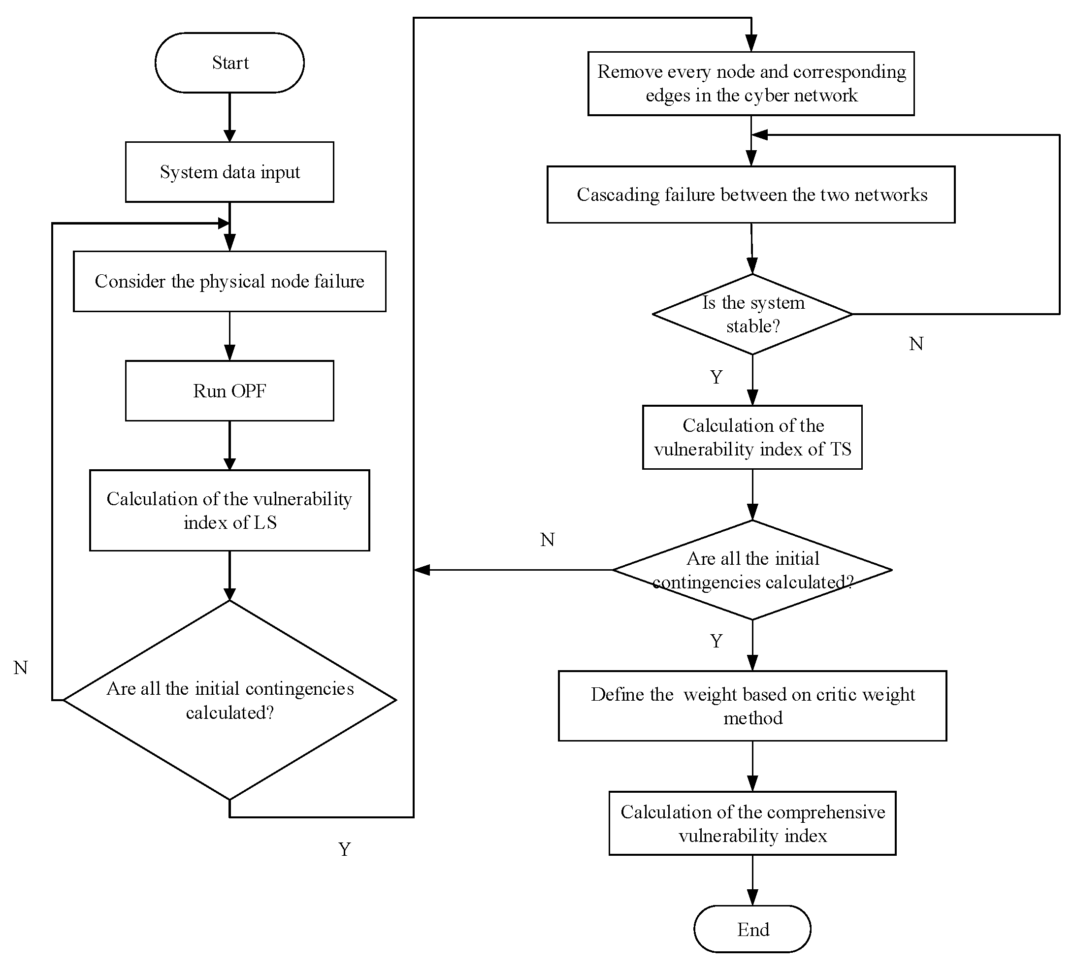
2.4. Comprehensive Vulnerability Index

Two indexes that contribute to vulnerability have been described. These indexes can be considered as a tuple that describes CPPS vulnerability. However, managers may prefer a single score, which allows them to know the status of the system. The critic weight method can be used to evaluate the importance of each index. Therefore, these indexes are integrated using a multi-criteria decision making (MCDM) problem framework. Each parameter is weighted by the critic weight method. After being normalized [2], the comprehensive vulnerability index (CVI) is calculated as follows:

$$CVI={\alpha }_1\times LSI+{\alpha }_2\times TSI$$

(17)

where ${\alpha }_1$ is the weight of $LSI$; ${\alpha }_2$ is the weight of $TSI$.

The integrative flow diagram of the vulnerability assessment scheme is provided in Figure 3.

3. Active and Passive Defense Strategies

3.1. Active Defense Strategy Based on Vulnerability Assessment

Exploring vulnerable parts and strengthening the communication network can realize preventive control when attacks do not occur (active defense). Active defense strategy for the operational plan is based on the vulnerability analysis of CPPS. Deploying some false nodes around certain nodes is an effective active strategy. Certain nodes are the true nodes high-ranking in vulnerability analysis. The nodes are very dangerous in that they may be attacked maliciously with a higher probability. If false nodes are attacked, a warning signal will be sent to the manager of the system. However, the attacker may skip the false nodes to real ones. False nodes deployed in CPPS are treated as decoys to attract attackers. It is a useful defense measure against various attacks [23]. It is assumed that the attacker can not distinguish between real nodes and false nodes. The purpose for deploying false nodes are listed as follows:

(1) Detract the attacker to avoid the real node being attacked;

(2) Attract the attacker to waste its resources to reduce the probability of real nodes being attacked.

Deploying false nodes is an effective method. It is necessary to assess and judge the amount and location of false nodes. To maximize the defend effect of false nodes, the number of false nodes around a true node is worth considering. When the ratio of true and false nodes is $1:N$. The probability that the first attack will be detected is $\frac{N}{1+N}$. The probability of successful attacking the real node and then being detected is $\frac{N}{{(1+N)}^2}$. The probability that no more than one real node fails due to a random attack is $\frac{N^2+N}{{(1+N)}^2}$.

It is noted that setting three false nodes can defend 94% attacks while it is 96% with four false nodes (Figure 4). It is wise to set three false nodes considering the cost.

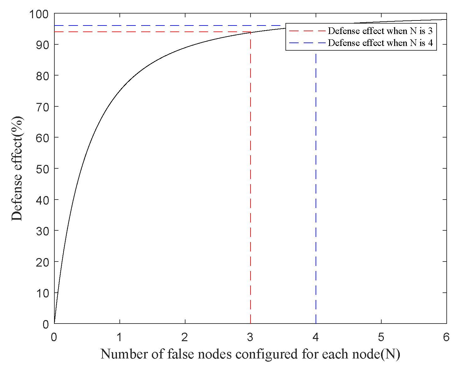
3.2. Passive Defense Strategy

It is inevitable that more and more nodes lose control once the system suffers attacks. The system may collapse without being repaired and corrected. Because active defense strategy may not always hold, control mode can change from centralized control to centralized-distributed control to recovery and correct nodes out of control.

Community structure is one of the characteristics of complex networks. The network can be divided into several communities. The relationships between nodes in the same community are close, and different communities are sparse. The cyber network is divided into several communities based on the Kernighan-link algorithm. The node with the largest degree is set as the distributed control node in every community.

There are several distributed control nodes whose control scope is limited in the cyber network. Distributed control nodes can only save the nodes linking to them. To recapitulate, a cyber node that can be corrected and repaired has to meet the following three conditions.

(1) The node is not belonging to the giant component, i.e., the node is out of control.

(2) The node is in the control scope of distributed control nodes, i.e., there exists an edge between the node and distributed control nodes at least.

(3) The node has the electricity support from the physical network, i.e, its corresponding node in the physical network survive in the stages before.

Choosing an edge of the network randomly leads to a node connected to the giant component, where f is:

$$f=\lambda (1-G_1(1-f))$$

(18)

where $G_1\left(x\right)={\sum }_{k=min}^{k=max}kp\left(k\right)/<k>x^{k-1}$ is the generating function of the excess degree distribution; $<k>$ is the average degree of the network; $\lambda$ is the fraction of remaining nodes. The fraction of survival nodes in the network is:

$$P_{\infty }\left(\lambda \right)=\lambda (1-G_0(1-f))$$

(19)

where $G_0\left(x\right)={\sum }_{k=k_{min}}^{k=k_{max}}P\left(k\right)x^k$ is the generating function of the degree distribution.

Attacking is simulated by removing some nodes in the cyber network. A fraction $S_C\left(0\right)={\lambda }_C\left(0\right)-{P_{\infty }}^C\left(0\right)$ of nodes will lose control and dysfunction without saving and correcting. Before the cascading failure spreads to the physical network, distributed control nodes will start repairing a fraction $R_C\left(0\right)$ of nodes that satisfy the conditions. Only a fraction ${S_C}^{\prime }\left(0\right)={\lambda }_C\left(0\right)-{P_{\infty }}^C\left(0\right)+R_C\left(0\right)$ of nodes fail under repairing and saving. Then, the failure spreads to the physical network and back and forth until it reaches a steady state. The strategy is applied when the failure in the cyber network propagates to the physical network and just before its return to the cyber network.

4. Case Study and Discussion

Scale-free (SF) network and small world (SW) network are two typical communication networks to analyze robustness and stability of the system. The experiments are made on the IEEE 118 busbar system (physical network). It is coupled with SF and SW to establish CPPS, separately. There are 123 nodes, including 118 normal nodes, 2 centralized control nodes, and 3 distributed control nodes in the cyber network. The ability of a single node to process information is proportional to its degree. The nodes with the largest and the second-largest degree are set as the centralized control nodes.The cyber network is divided into three communities according to Kernighan–Lin algorithm.The node with the largest degree in every community is set as the distributed control node. There are several types of attacks defined as follows:

(1) Random attack: select cyber nodes randomly as attacking targets;

(2) High degree attack: rank cyber nodes by degree and select nodes as attacking targets from high to low;

(3) High betweenness attack: rank cyber nodes by betweenness and select nodes as attacking targets from high to low;

(4) High CVI attack: rank cyber nodes by the proposed comprehensive vulnerability index and select nodes as attacking targets from high to low.

It is assumed that central control nodes and distributed control nodes will not be attacked successfully because they generally have special protection equipment due to their vital status.

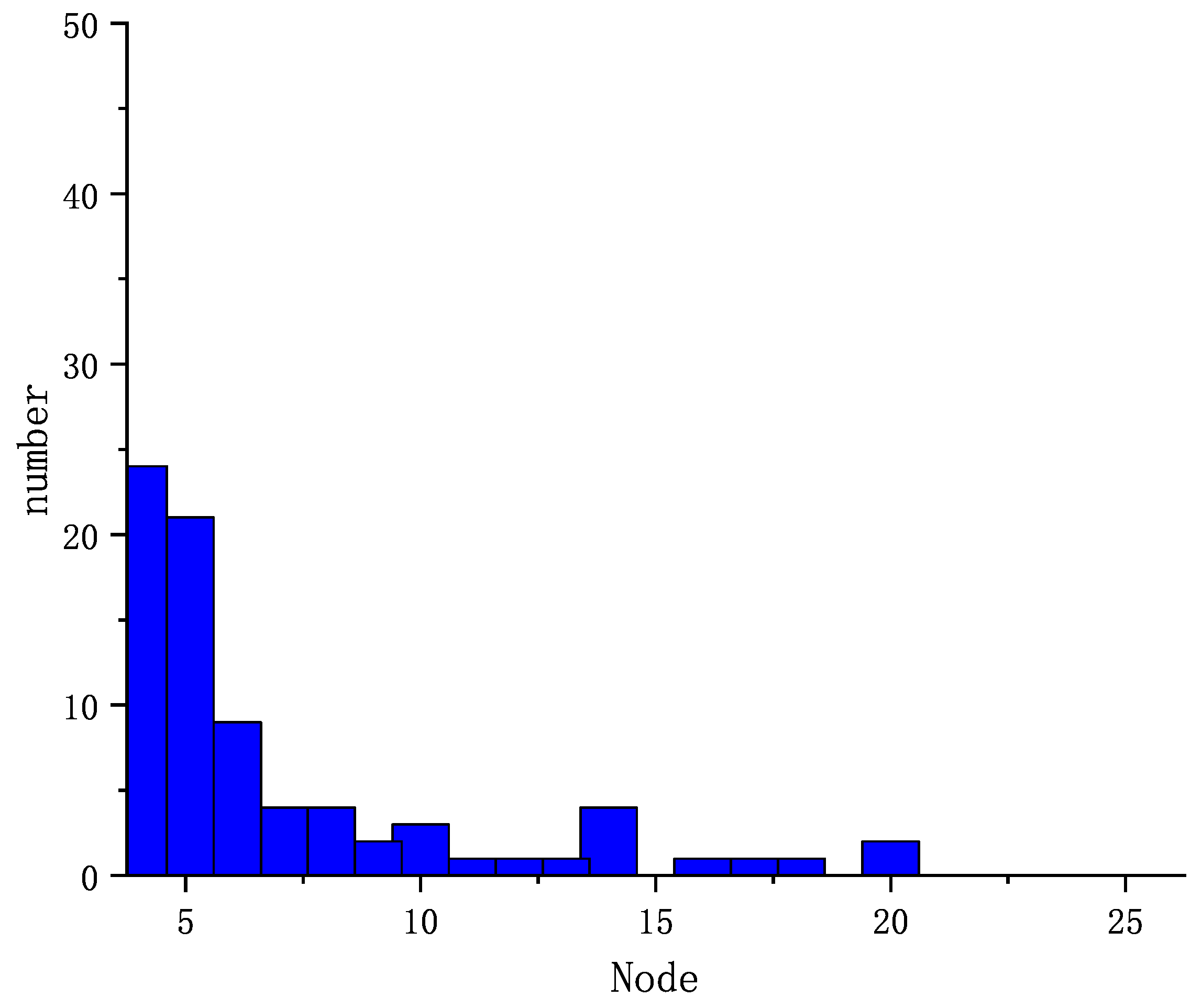
4.1. Scale-Free (SF) Network

SF network (Figure 5) is generated according to the corresponding algorithm [24]. It is molded with $T=123$, $m_0=3$, and $m=3$ where,

T is the final number of new nodes;

m is the number of connections to existing nodes when a new node is generated to construct the network;

$m_0$ is the number of nodes at the beginning.

Node 1 and 4 are set as centralized control nodes. Nodes 2, 3, and 78 are set to be distributed control nodes.

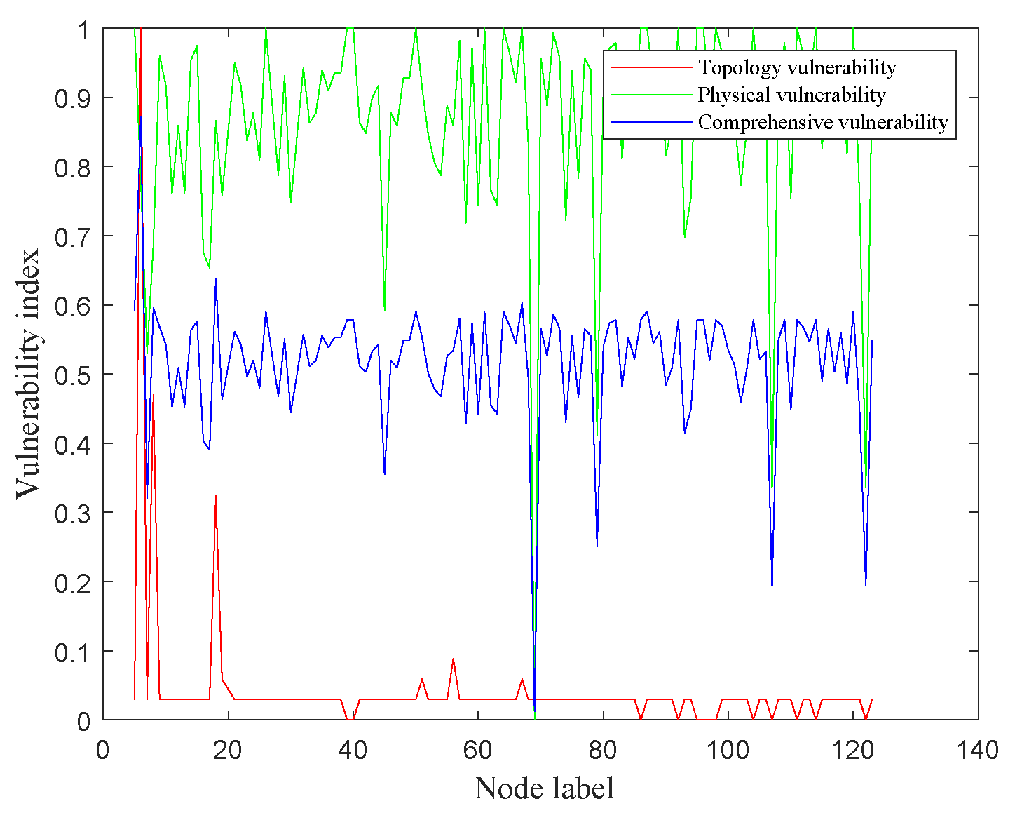
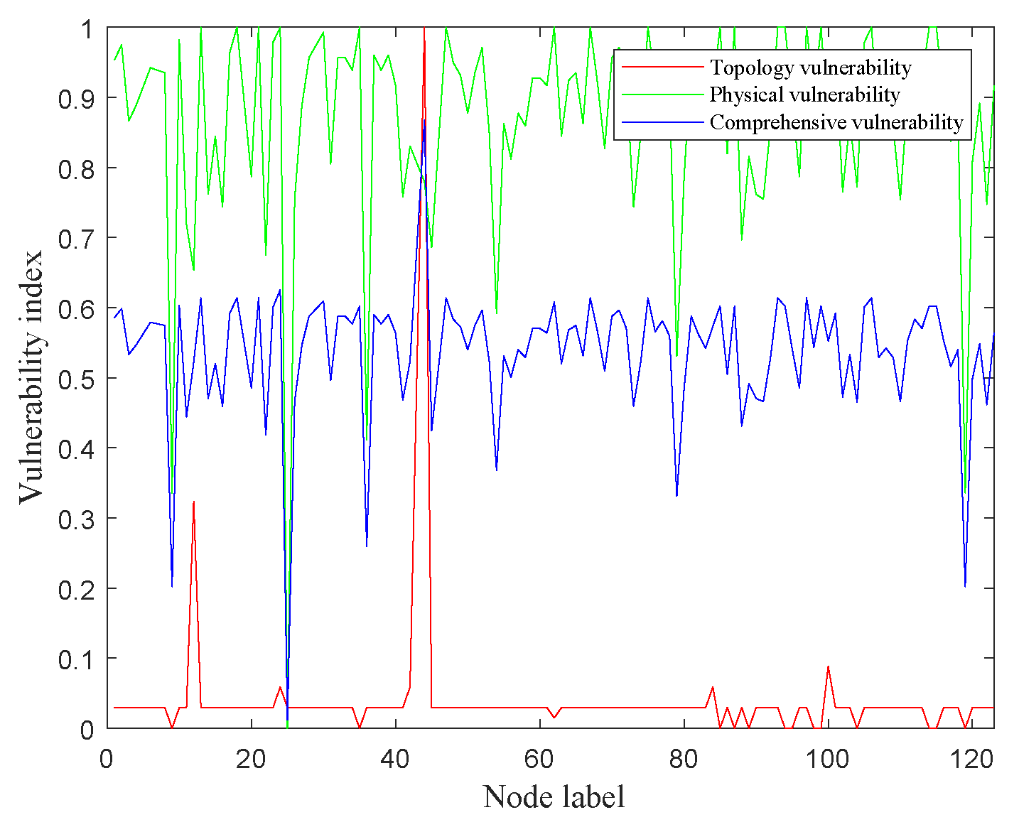
4.1.1. Result 1: Vulnerability Assessment and Deploying False Nodes Based on the Comprehensive Vulnerability Index

To explore the vulnerable nodes in the cyber network, the vulnerability of every node is assessed according to Figure 3. ${\alpha }_1$ is 0.4219 and ${\alpha }_2$ is 0.5781 according to Equation (17).

It is apparent from Figure 6 that there are still many differences between nodes despite the N − 1 principle in the power grid. It is reasonable to adopt CVI as a vulnerability index.

The data of the top 20 nodes based on CVI are listed in

Table 3. Vulnerability indexes of Top 20 nodes.

Node	Physical Index	Topology Index	CVI	Node	Physical Index	Topology Index	CVI
6	0.779783	1	0.872693	120	1	0.029412	0.590509
18	0.866426	0.323529	0.637378	72	0.99278	0.029412	0.586335
67	1	0.058824	0.602918	57	0.981949	0.029412	0.580074
8	0.685921	0.470588	0.595072	39	1	0	0.5781
5	1	0.029412	0.590509	40	1	0	0.5781
26	1	0.029412	0.590509	86	1	0	0.5781
50	1	0.029412	0.590509	92	1	0	0.5781
61	1	0.029412	0.590509	95	1	0	0.5781
64	1	0.029412	0.590509	96	1	0	0.5781
87	1	0.029412	0.590509	98	1	0	0.5781

. As shown in Table 3, physical vulnerability and topology vulnerability do not match exactly, e.g., node 61 has a high physical vulnerability of 1, but low topology vulnerability of 0.029412. The degrees of node 61 and its corresponding node in the physical network are three. Attacking node 61 may not result in great losses in topology. However, its corresponding node 61 is a generator node whose active capacity is 160. Large active power will result in great losses in the physical aspect. It can not provide an accurate and practical index only considering physical properties or system structure. The comprehensive vulnerability index can assess the vulnerability considering both of them.

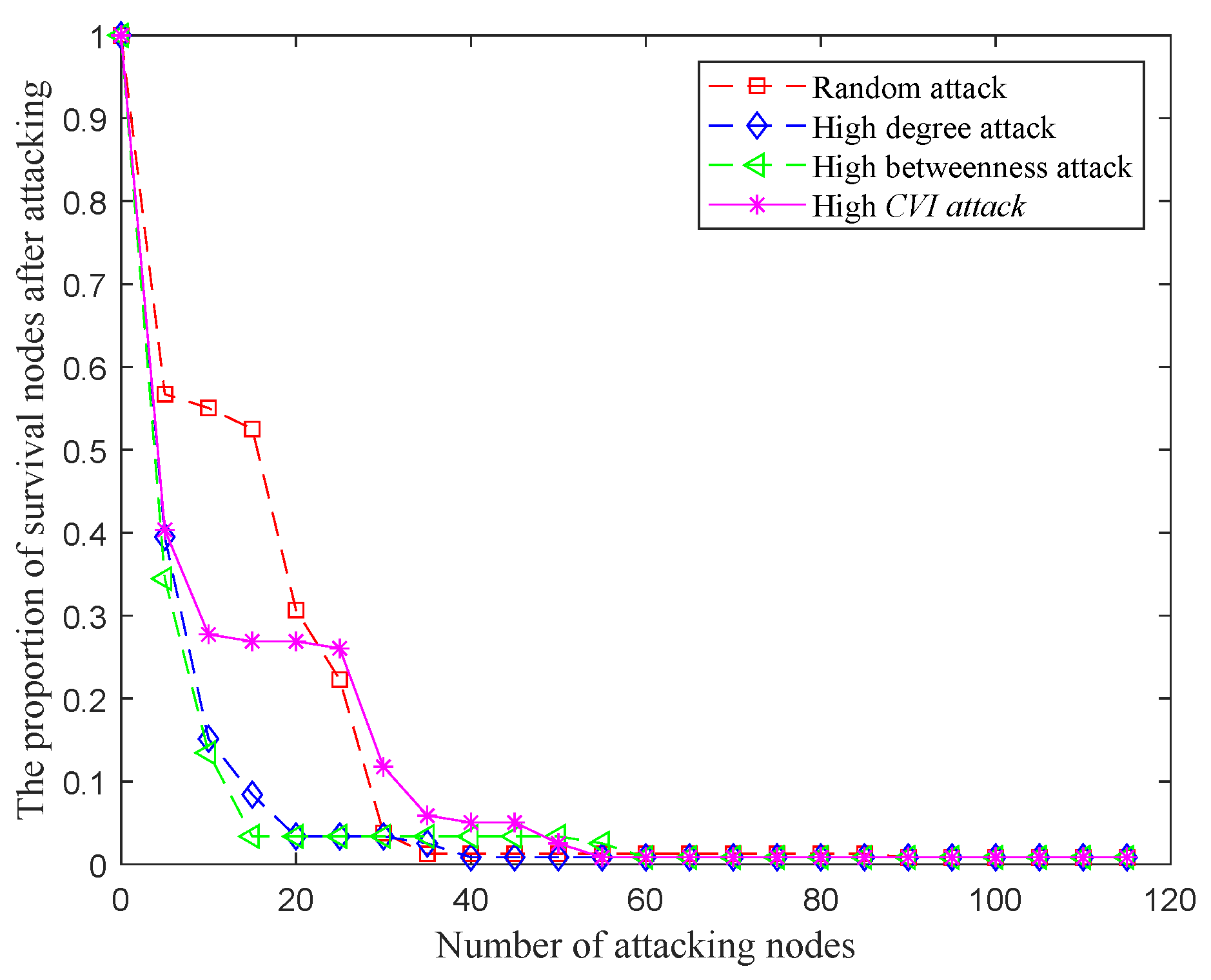
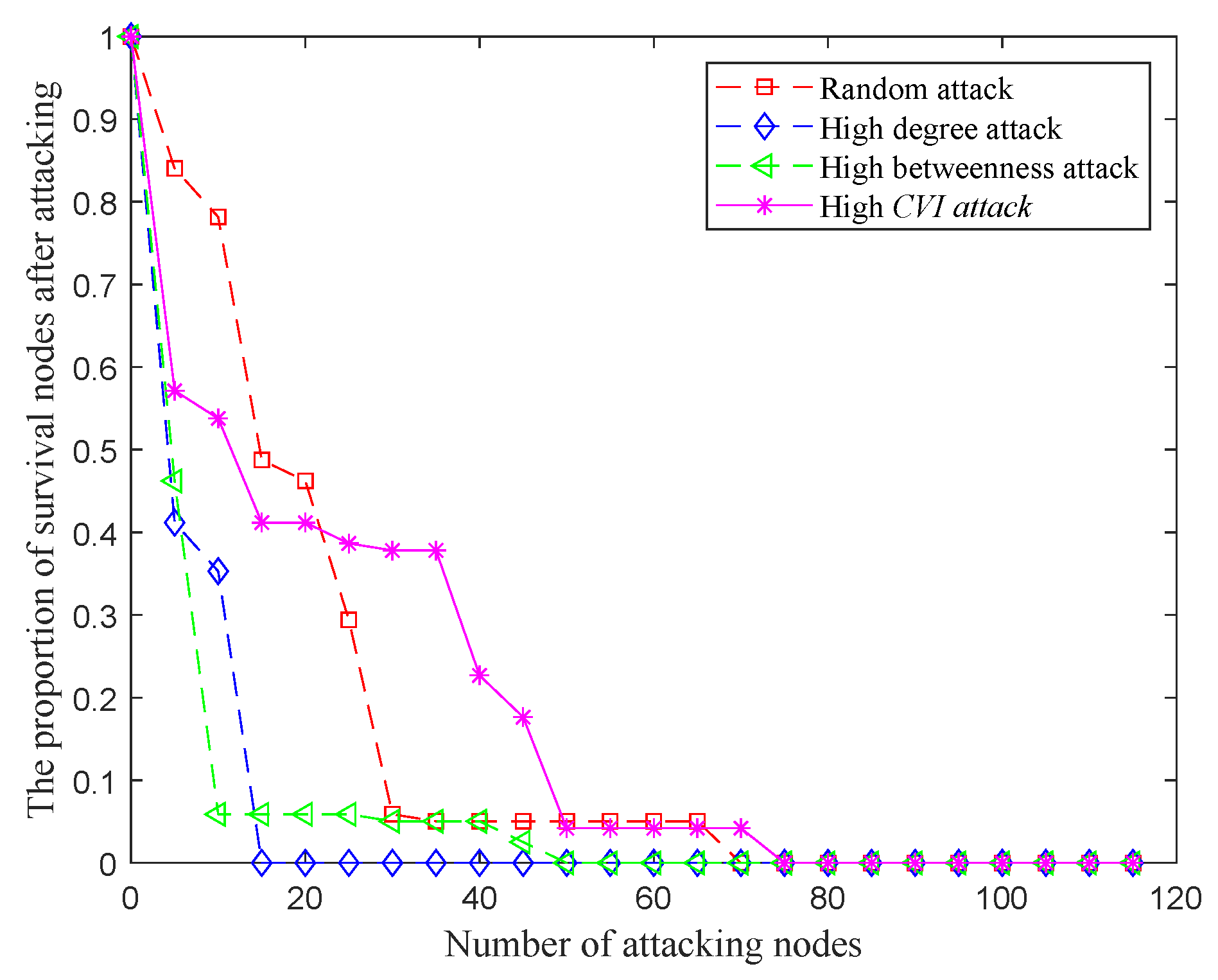
4.1.2. Nodes Survived under Different Types of Attacks

To investigate how CPPS is affected by different attacks, the system is attacked by random attack, high degree attack, high betweenness attack, and high CVI attack separately (Figure 7). The survival nodes are calculated. With the increasing number of attacking nodes, there is the first-order percolation in the system for certain, i.e., there exists a threshold. If the number of attacking nodes excesses the certain threshold, the system will collapse that nearly all nodes are out of control. The threshold can be an important metric to test the robustness of the system. The proportion of survival nodes remains low and does not change much as the number of attacking nodes increases. At this time, it is assumed that the system reaches the threshold. The thresholds of different attacks are listed in

Table 4. The thresholds of different attacks.

Type	Random Attack	High Degree Attack	High Betweeness Attack	High CVI Attack
Threshold	35	20	15	40

.

Figure 7 suggests that the system is the most vulnerable under high degree attacks and high betweenness attacks. The system is comparably robust under random attacks that attacking nearly 35% of nodes can make the system collapse. Despite the damage to CPPS under CVI attack is less serious, CVI is combing physical characteristics and topology. It may cause more losses in reality.

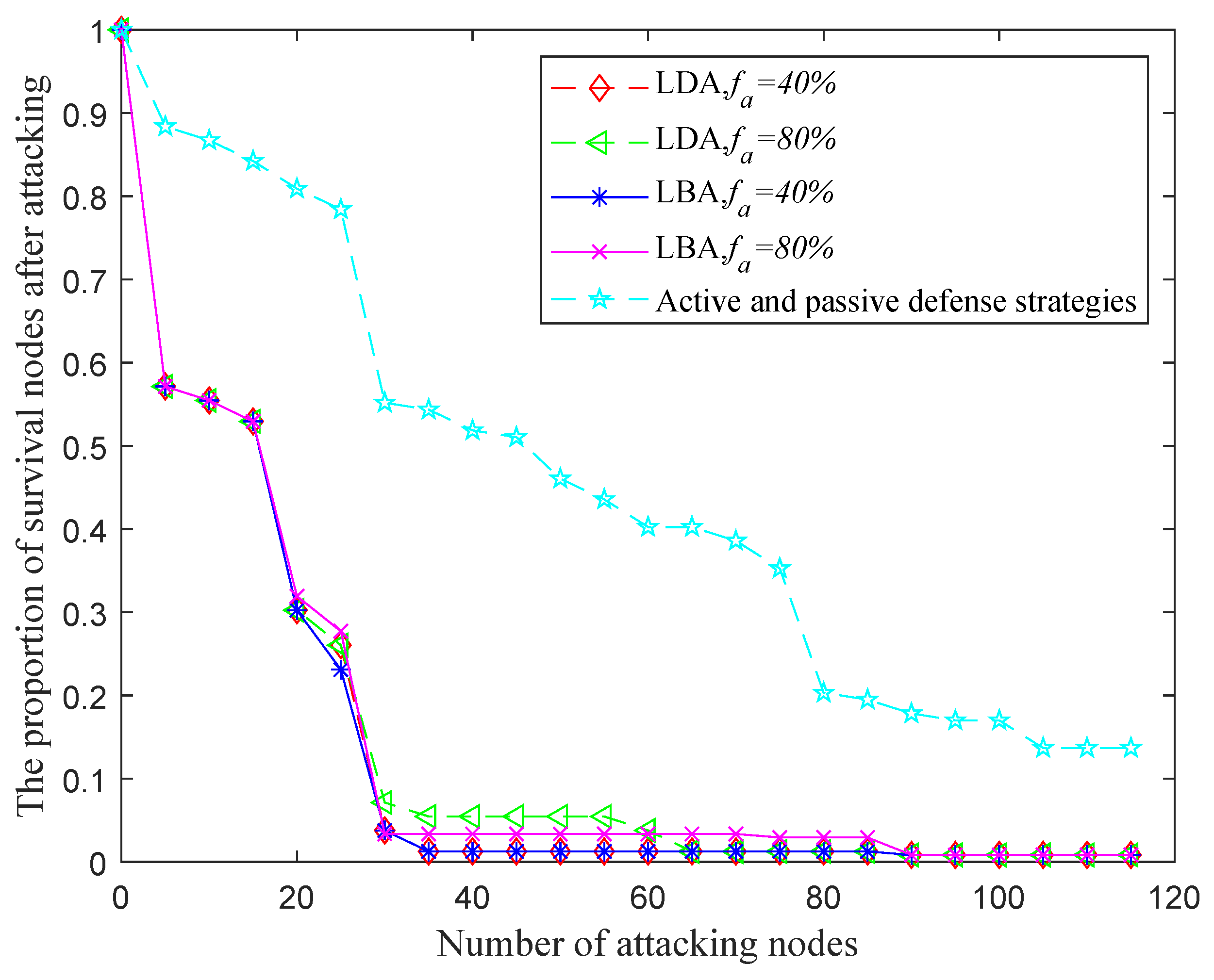
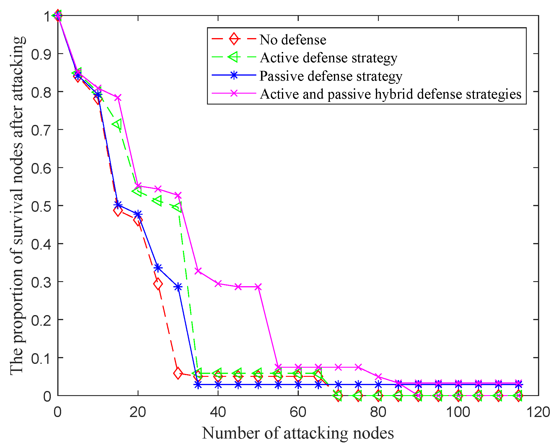
4.1.3. The Effect of the Active and Passive Hybrid Stategies

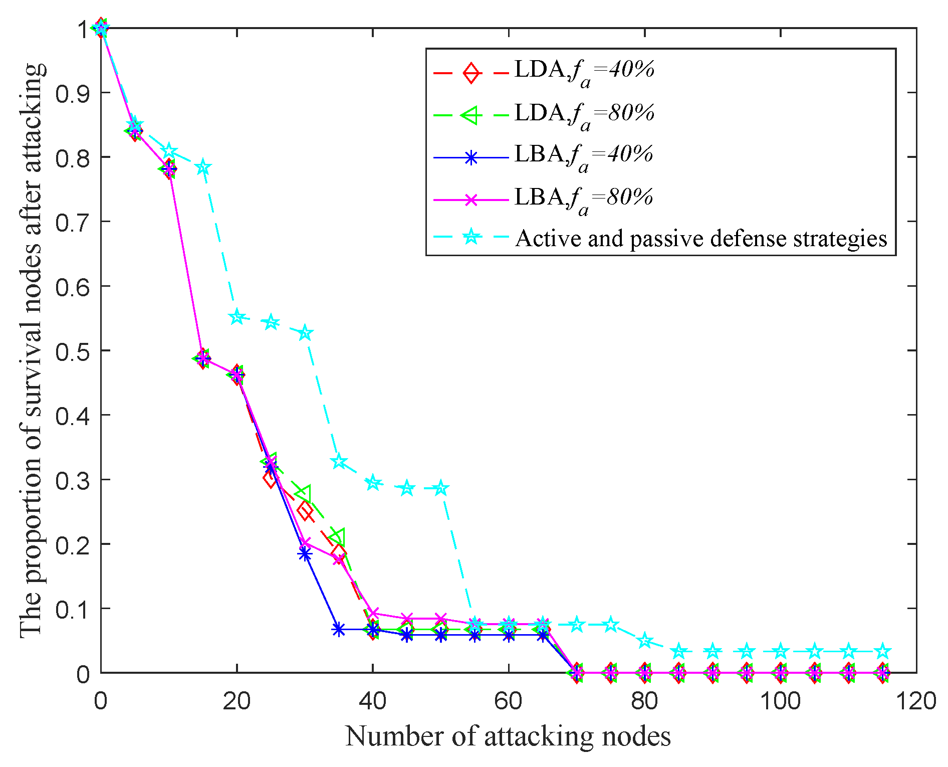
To validate the protection effect with active and passive strategies, attacking is simulated under random attack with active and passive strategies (Figure 8). The top twenty percent of CVI nodes are deployed with false nodes.

Statistics of survival nodes are presented in

Table 5. The propotion of survival nodes.

Different Situations	Attacking Nodes
	10	20	30	40	50	60	70	80	90	100
No defense	0.5504	0.3067	0.0378	0.0126	0.0126	0.0126	0.0126	0.0126	0.0084	0.0084
Active defense	0.5588	0.5	0.2143	0.2143	0.1555	0.1471	0.1303	0.1050	0.0630	0.0630
Passive defense	0.8672	0.6763	0.3527	0.2946	0.2780	0.2282	0.2199	0.1037	0.0996	0.0830
Active and passive hybrid defense	0.8672	0.8091	0.5519	0.5187	0.4606	0.4025	0.3859	0.2033	0.1784	0.1701

. As shown in Table 5, the defense effect of false nodes is obvious in the middle stages (20–40). As the number of attacking nodes increase, it becomes less useful. Another observation is that the change from centralized control mode to centralized-distributed control mode is effective during the initial and middle period (10-70). However, the active defense strategy can not prevent the first-order percolation. It is exciting to observe that the first-order percolation disappeared under the active and passive hybrid defense strategies. As the number of attacking nodes increases, the effect of the hybrid defense strategies becomes more obvious. The robustness and vulnerability of the system are greatly improved and the system can be controlled properly.

Traditional methods to enhance robustness of internetwork are adding edges between some vulnerable nodes in topology. To illustrate the superiority of our method, a comparison of the results of different methods has been made. Our methods are compared with adding edges between low degree nodes and low-betweenness nodes. Two methods of adding edges are defined as follows:

•

Low Degree Nodes Link Addition (LDA): At each step, the node degree of the network is calculated and two nodes with the lowest degree are added with an edge. Repeat the algorithm until the specified number of added edges is reached.

•

Low Betweenness Nodes Link Addition (LBA): At each step, the node betweenness of the network is calculated and two nodes with the lowest betweenness are added with an edge. Repeat the algorithm until the specified number of added edges is reached.

The proportion of adding is calculated as:

$$f_a=\frac{N_a}{N_{OR1}+N_{OR2}}$$

(20)

where, $N_a$ is the number of adding edges;

$N_{OR1}$ is the edge number of the original cyber network;

$N_{OR2}$ is the edges number of the original physical network.

Compared to traditional methods, active and passive defense strategies are more effective comparably (Figure 9). The robustness of the system is greatly improved. With the increase of the number of attacking nodes, the advantages of the traditional method gradually appeared. However, the effect of active and passive defense strategies are more obvious comparably.

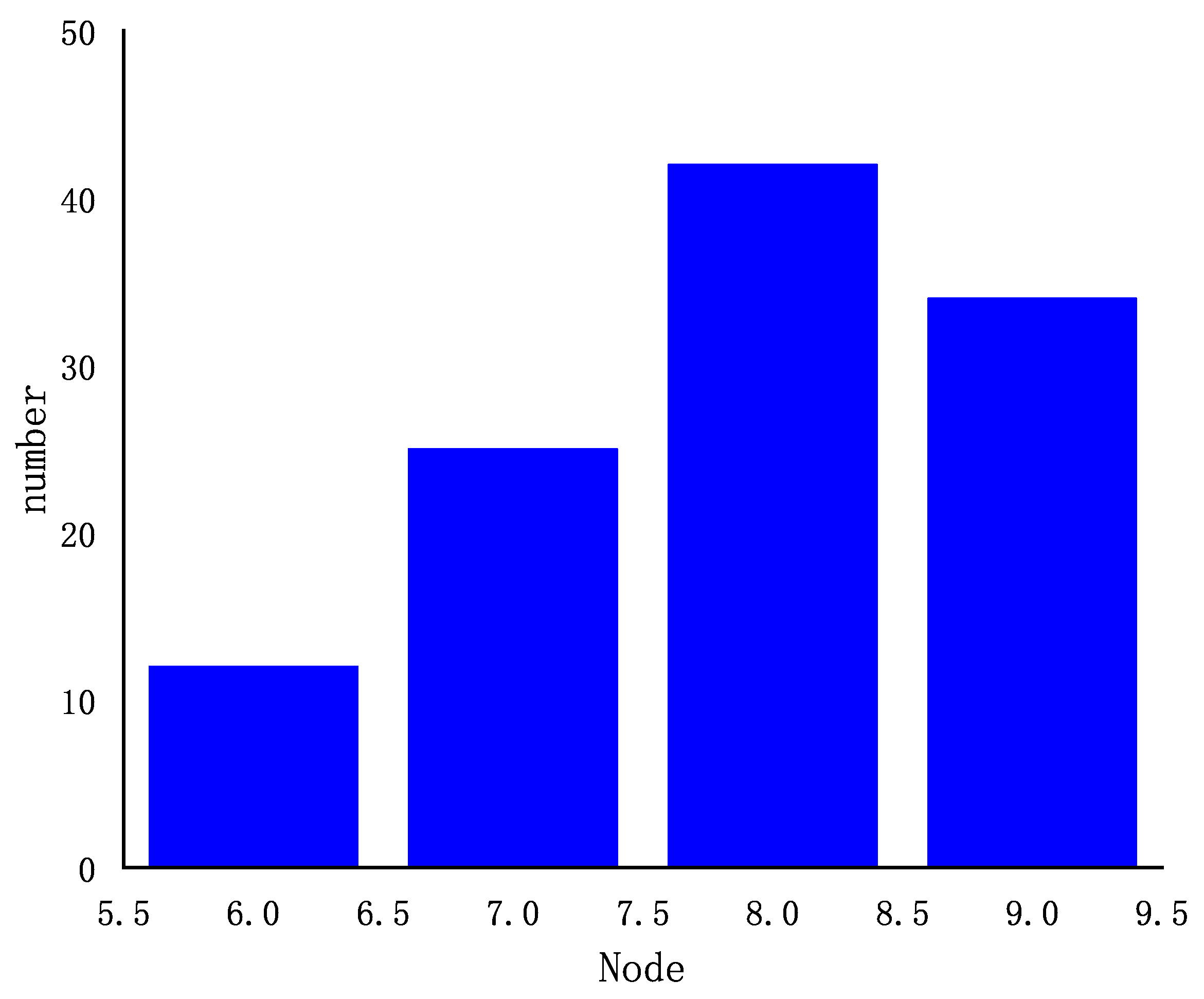
4.2. Small World (SW) Network

SW network (Figure 10) is generated according to the corresponding algorithm [25]. The network is set as follows: k is 6; p is 0.2. Node 5 and 19 are set as central control nodes. Node 29, 43, and 46 are set as distributed control nodes. ${\alpha }_1$ is 0.6021 and ${\alpha }_2$ is 0.3979 according to Equation (17).

4.2.1. Result 1: Vulnerability Assessment and Deploying False Nodes Based on the Comprehensive Vulnerability Index

It is apparent from Figure 11 that the vulnerability of different nodes varies considerably. As shown in

Table 6. Vulnerability Indexes of Top 20 nodes.

Node	Physical Index	Topology Index	CVI	Node	Physical Index	Topology Index	CVI
44	0.779783	1	0.867408	30	0.99278	0.029412	0.609456
3	0.866426	0.323524	0.650407	10	0.981949	0.029412	0.602935
24	1	0.058824	0.625506	35	1	0	0.6021
13	1	0.029412	0.613803	67	1	0	0.6021
18	1	0.029412	0.613803	85	1	0	0.6021
21	1	0.029412	0.613803	93	1	0	0.6021
47	1	0.029412	0.613803	94	1	0	0.6021
62	1	0.029412	0.613803	97	1	0	0.6021
75	1	0.029412	0.613803	99	1	0	0.6021
87	1	0.029412	0.613803	106	1	0	0.6021

, physical vulnerability and topology vulnerability do not match exactly, e.g., node 62 has a high physical vulnerability 1 but low topology vulnerability 0.029412. The degree of node 62 is 9 and the degree of its corresponding node 103 is 4. Attacking node 62 may not result in great losses in topology. However, its corresponding node 103 is a generator node whose active capacity is 40. Large active power will result in great losses in the physical aspect.

4.2.2. Nodes Survived under Different Types of Attacks

The system is still attacked by random attack, high degree attack, high betweenness attack, and high CVI attack (Figure 12). What stands out in the figure is that the SW network is more vulnerable under attacks. The system has collapsed under 10 high betweenness attacks. The threshold is 30 if under random attacks.

4.2.3. The Effect of the Active and Passive Stategies

It is crucical to enhance the robustness of such a system. Attacking is simulated under random attacks with active and passive defense strategies (Figure 13). The CVI top 20% are deployed with false nodes. As shown in Figure 13, the protection effect is apparent in the SW network, e.g., the threshold has risen from 30 to 55 under hybrid defense strategies. Statics of survival nodes is presented in

Table 7. The propotion of survival nodes.

Different Situations	Attacking Nodes
	10	20	30	40	50	60	70	80	90	100
No defense	0.7815	0.4622	0.0588	0.0504	0.0504	0.0504	0	0	0	0
Active defense	0.7983	0.5378	0.4958	0.0588	0.0588	0.0588	0	0	0	0
Passive defense	0.7925	0.4772	0.2863	0.029	0.029	0.029	0.029	0.029	0.029	0.029
Active and passive hybrid defense	0.8091	0.5519	0.5270	0.2946	0.2863	0.0747	0.0747	0.0498	0.0332	0.0332

. The comparison of the traditional method and hybrid defense strategies are shown in Figure 14.

4.3. Comparision and Discussion

The single most conspicuous observation to emerge from the results is that there exists a first-order percolation when the number of attacking nodes up to a certain threshold, in agreement with results from [12]. However, the first-order percolation disappears under the active and passive defense strategy in the SF network, while the SW network transfers from the first-order percolation to the second-order percolation. Comparison of the findings with SW or scale-free network shows that small world network is more vulnerable. This discrepancy could be attributed to the topology structure. In SW, the degrees of all nodes are approximately equal (Figure 15) and the nodes have a large clustering coefficient of 0.4213. Clustering coefficients represent the level of connection between nodes. As shown in Figure 16, the scale-free network is an exponential network that a few nodes have numerous connections. The clustering coefficient tends to be 0 when the network scale is large enough. It is somewhat surprising that scale-free networks are robust to random failures, but vulnerable to intentional attacks. The root of this phenomenon is that scale-free networks have a certain proportion of high degree nodes and the degree of the most nodes are very low (Figure 16). The nodes are not tightly enough connected that the system collapses easily when high degree nodes suffer intentional attacks.

Our study provides additional support for considerable insight into CPPS defending. Deploying false nodes can postpone the system collapsing in the initial period. A possible explanation for this might be that only some vulnerable nodes are deployed false nodes. This method can be useful when there is a small number of nodes under attack. As the number of attacking nodes increases, this method alone cannot protect the system well. Countermeasures must be taken immediately. In the middle period, distributed control nodes can protect the system well. Its effect is obvious with the increasing of attacking nodes. Accomplishing centralized-distributed control, the system is robust even suffering numerous attacks. The first-order percolation disappears in the SF network and the SW network transfers from the first-order percolation to the second-order percolation. This discrepancy could be attributed to their community structure and degree distribution. The Q of the SW network is 0.4467, while Q is 0.2621 in the SF network. The higher the index Q represents the closer the connection between nodes in one community. The failure of one node can propagate to larger areas, while distributed control nodes can only repair and correct certain nodes. A wide range of degree distribution makes it so distributed control nodes can correct more nodes in the SF network.

5. Conclusions

The system robustness is tested under different attacks in the cyber network and active and passive strategies are established. Based on the comprehensive vulnerability index, some of the most vulnerable nodes are deployed with false nodes as the active defense. Adopting distributed control nodes is set as the passive defense. Combined with active and passive strategies, the robustness of the system can be improved greatly.

The main findings are as follows:

(a) Due to differences in vulnerability, the robustness of SW and scale-free networks react differently under numerous attacks. Even the same network shows different robustness under different attacks. This conclusion should, therefore, be of value for constructing communication networks in reality.

(b) On the basis of the results, the effect of active and passive defense strategies is more obvious in the SF network than the SW network. The first-order percolation disappears under active and passive defense strategy in the SF network, while the SW network transfers from the first-order percolation to the second-order percolation.

(c) Active and passive strategies function at different periods. Based on active and passive strategies, CPPS can defend against numerous attacks and the robustness of the system can be enhanced dramatically.

However, our study still has some limitations, which can be improved in the future work. There is an optimal solution for how many real nodes are deployed with false nodes considering the defend effect and cost. Furthermore, the islanding power grid should be considered in the future research. Further experimental studies are needed to explore intentional islanding in the grid.

References

1. Zonouz, S.; Rogers, K.M.; Berthier, R.; Bobba, R.B.; Sanders, W.H.; Overbye, T.J. SCPSE: Security-Oriented Cyber-Physical State Estimation for Power Grid Critical Infrastructures. IEEE Trans. Smart Grid 2012, 3, 1790–1799. [Google Scholar] [CrossRef]
2. Dobson, I.; Carreras, B.A.; Lynch, V.E.; Newman, D.E. Complex systems analysis of series of blackouts: Cascading failure, critical points, and self-organization. Chaos 2007, 17, 967–979. [Google Scholar] [CrossRef] [PubMed]
3. Zheng, Y.; Yan, Z.M.; Chen, K.J.; Sun, J.W.; Xu, Y.; Liu, Y. Vulnerability Assessment of Deep Reinforcement Learning Models for Power System Topology Optimization. IEEE Trans. Smart Grid 2021, 12, 3613–3623. [Google Scholar] [CrossRef]
4. Gao, X.L.; Pu, C.L.; Li, L.B. Vulnerability Assessment of Power Grids Against Cost-Constrained Hybrid Attacks. IEEE Trans. Circuits Syst. II Express Briefs 2021, 68, 1477–1481. [Google Scholar] [CrossRef]
5. Venkataramanan, V.; Hahn, A.; Srivastava, A. CP-SAM: Cyber-Physical Security Assessment Metric for Monitoring Microgrid Resiliency. IEEE Trans. Smart Grid 2020, 11, 1055–1065. [Google Scholar] [CrossRef]
6. Liu, N.A.; Hu, X.J.; Ma, L.; Yu, X.H. Vulnerability Assessment for Coupled Network Consisting of Power Grid and EV Traffic Network. IEEE Trans. Smart Grid 2022, 13, 589–598. [Google Scholar] [CrossRef]
7. Ding, K.; Qian, Y.M.; Wang, Y.; Hu, P.; Wang, B. A Data-Driven Vulnerability Evaluation Method in Grid Edge Based on Random Matrix Theory Indicators. IEEE Access 2020, 8, 26495–26504. [Google Scholar] [CrossRef]
8. Ibrahim, M.; Alsheikh, A. Automatic Hybrid Attack Graph (AHAG) Generation for Complex Engineering Systems. Processes 2019, 7, 787. [Google Scholar] [CrossRef] [Green Version]
9. Ni, Z.; Paul, S. A Multistage Game in Smart Grid Security: A Reinforcement Learning Solution. IEEE Trans. Neural Netw. Learn. Syst. 2019, 30, 2684–2695. [Google Scholar] [CrossRef]
10. Venkataramanan, V.; Srivastava, A.; Hahn, A. Cp-tram: Cyber-physical transmission resiliency assessment metric. IEEE Trans. Smart Grid 2020, 11, 5114–5123. [Google Scholar] [CrossRef]
11. Hu, P.; Lee, L. Community-Based Link-Addition Strategies for Mitigating Cascading Failures in Modern Power Systems. Processes 2020, 8, 126. [Google Scholar] [CrossRef] [Green Version]
12. Yagan, O.; Qian, D.J.; Zhang, J.S.; Cochran, D. Optimal Allocation of Interconnecting Links in Cyber-Physical Systems: Interdependence, Cascading Failures and Robustness. IEEE Trans. Parallel Distrib. Syst. 2012, 23, 1708–1720. [Google Scholar] [CrossRef] [Green Version]
13. Huang, Z.; Wang, C.; Stojmenovic, M.; Nayak, A. Characterization of cascading failures in interdependent cyber-physical systems. IEEE Trans. Comput. 2015, 64, 2158–2168. [Google Scholar] [CrossRef]
14. Ji, X.; Wang, B.; Liu, D.C.; Dong, Z.Y.; Chen, G.; Zhu, Z.S.; Zhu, X.D.; Wang, X.T. Will electrical cyber-physical interdependent networks undergo firstorder transition under random attacks? Phys. A Stat. Mech. Appl. 2016, 460, 235–245. [Google Scholar] [CrossRef]
15. Wang, K.; Du, M.; Maharjan, S.; Sun, Y.F. Strategic Honeypot Game Model for Distributed Denial of Service Attacks in the Smart Grid. IEEE Trans. Smart Grid 2017, 8, 2474–2482. [Google Scholar] [CrossRef]
16. Zhou, H.F.; Wu, C.M.; Jiang, M.; Zhou, B.Y.; Gao, W.; Pan, T.T.; Huang, M. Evolving defense mechanism for future network security. IEEE Commun. Mag. 2015, 53, 45–51. [Google Scholar] [CrossRef]
17. Ni, M.; Li, M.L.; Li, J.; Wu, Y.J.; Wang, Q. Concept and Research Framework for Coordinated Situation Awareness and Active Defense of Cyber-physical Power Systems Against Cyber-attacks. Mod. Power Syst. Clean Energy 2021, 9, 477–484. [Google Scholar] [CrossRef]
18. Farraj, A.; Hammad, E.; Kundur, D. A Distributed Control Paradigm for Smart Grid to Address Attacks on Data Integrity and Availability. IEEE Trans. Signal Inf. Process. Over Netw. 2017, 4, 70–81. [Google Scholar] [CrossRef]
19. Di Muro, M.A.; La Rocca, C.E.; Stanley, H.E.; Havlin, S.; Braunstein, L.A. Recovery of Interdependent Networks. Sci. Rep. 2016, 6, 22834. [Google Scholar] [CrossRef]
20. La Rocca, C.E.; Stanley, H.E.; Braunstein, L.A. Strategy for for stopping failure cascades in interdependent networks. Phys. Stat. Mech. Appl. 2018, 508, 577–583. [Google Scholar] [CrossRef] [Green Version]
21. Gao, Z.; Liu, X. An Overview on Fault Diagnosis, Prognosis and Resilient Control for Wind Turbine Systems. Processes 2021, 9, 300. [Google Scholar] [CrossRef]
22. Parshani, R.; Rozenblat, C.; Ietri, D.; Ducruet, C.; Havlin, S. Intersimilarity between coupled networks. Europhys. Lett 2010, 92, 68002. [Google Scholar] [CrossRef] [Green Version]
23. Levitin, G.; Hausken, K.; Ben Haim, H. False Targets in Defending Systems against Two Sequential Attacks. Mil. Oper. Res. J. Mil. Oper. Res. Soc. 2014, 19, 19–35. [Google Scholar] [CrossRef]
24. Barabási, A.; Albert, R. Emergence of scaling in random networks. Science 1999, 286, 186–197. [Google Scholar] [CrossRef] [Green Version]
25. Watts, D.J.; Strogatz, S.H. Collective dynamics of ’small-world’networks. Nature 2011, 393, 301–303. [Google Scholar]
Figure 1. Cyber-physical power system.
Processes 10 01351 g001
Figure 2. Cyber network.
Processes 10 01351 g002
Figure 3. Flow chart of vulnerability assessment.
Processes 10 01351 g003
Figure 4. The effect of false nodes with a different number.
Processes 10 01351 g004
Figure 5. Scale-free network.
Processes 10 01351 g005
Figure 6. Vulnerability assessment of SF network.
Processes 10 01351 g006
Figure 7. Nodes survived under different attacks.
Processes 10 01351 g007
Figure 8. The effect of active and passive defense strategies.
Processes 10 01351 g008
Figure 9. Comparision active and passive defense strategies with traditional method.
Processes 10 01351 g009
Figure 10. Small world network.
Processes 10 01351 g010
Figure 11. Vulnerability assessment of small world network.
Processes 10 01351 g011
Figure 12. Nodes survived under different attacks.
Processes 10 01351 g012
Figure 13. The effect of active and passive defense strategies.
Processes 10 01351 g013
Figure 14. Comparison active and passive defense strategies with adding edges.
Processes 10 01351 g014
Figure 15. Degree distribution of SW network.
Processes 10 01351 g015
Figure 16. Degree distribution of SF network.
Processes 10 01351 g016