Abstract
The use of wind power generation can reduce the pollution in the environment and solve the problem of power shortages on offshore islands, grasslands, pastoral areas, mountain areas, and highlands. Wind speed forecasting plays a significant role in wind farms. It can improve economic and social benefits and make an operation schedule for wind turbines on large wind farms. This paper proposes a combined model based on the existing artificial neural network algorithms for wind speed forecasting at different heights. We first use the wavelet threshold method with the original wind speed dataset for noise reduction. After that, the three artificial neural networks, extreme learning machine (ELM), Elman neural network, and Long Short-term Memory (LSTM) neural network, are applied for wind speed forecasting. In addition, the variance reciprocal method and social cognitive optimization (SCO) algorithm are used to optimize the weight coefficients of the combined model. In order to evaluate the forecasting performance of the combined model, we select wind speed data at three heights (20 m, 50 m and 80 m) at the National Wind Technology Center M2 Tower. The experimental results show that the forecasting performance of the combined model is better than the single model, and it has a good forecasting performance for the wind speed at different heights.
1. Introduction
Wind energy, an essential renewable green energy source, has large reserves and wide distribution and has been widely used in many fields. At present, wind power generation is the emphasis of wind energy utilization. The latest released wind power data by the World Wind Energy Association revealed that the worldwide wind capacity reached approximately 744 gigawatts in 2020, wherein an unprecedented 93 gigawatts were added [1]. There are many advantages to wind power generation. It can reduce the pressure brought by the shortage of traditional energy and make a significant contribution to local life and development. Wind speed is the direct manifestation of wind energy, and accurate wind speed forecasting has a great significance. Therefore, it is the current research priority.
However, there is some trouble obtaining a high accuracy of wind speed forecasting results due to the random fluctuations of wind speed data caused by weather factors. Researchers have proposed a variety of methods for wind speed forecasting, including the statistical method, the physical method, the ANN method [2,3], and support vector machines (SVM) [4]. The statistical forecasting method is a method based on actual historical data; theoretical knowledge; and mathematical models to make quantitative forecasts about the development of things, mainly including the trend extrapolation method, the regression forecasting method [5], the Delphi method [6], the subjective probability method, the exponential smoothing (ES) method [7,8], the autoregressive integrated moving average (ARIMA) [9], the fuzzy system (FS) method [10], and other methods. Singh et al. [11] proposed a new Repeated wavelet transform- (WT) based ARIMA (RWT-ARIMA) model, which has improved accuracy for very short-term wind speed forecasting. Liu et al. [12] proposed a hybrid model based on empirical mode decomposition, novel recurrent neural networks and the ARIMA, in which ARIMA is employed to predict the low frequency sub-sequences and one residual.
The artificial neural network is a commonly used method due to its particular strengths in regression and classification. At the time of forecasting, the BP neural network and the Elman neural network are frequently used algorithms. Altan et al. [13] developed a new WSF model based on a long short-term memory (LSTM) network and decomposition methods with the grey wolf optimizer (GWO). Zhang et al. [14] proposed a novel model based on VMD-WT and PCA-BP-RBF neural networks for short-term wind speed forecasting. Catalão et al. [15] used a wavelet transform and an artificial neural network to forecast wind speed data for Portugal. Later, with mature technology, the researchers proposed the combination forecasting model and the hybrid forecasting model for wind speed forecasting. Many experimental results showed that the combination forecasting and hybrid forecasting models could improve forecasting accuracy and stability. Determining the appropriate weight coefficients is a critical step to obtaining better forecasting results. Compared to the method of using the algorithms to determine the weight coefficients directly, the method of using the modern intelligent optimization algorithms, such as the genetic algorithm (GA) [16] and the particle swarm optimization algorithm (PSO), [17] to further optimize the weight coefficients is more conducive to obtaining accurate results. Li et al. [18] proposed a combination model based on variable weight for wind speed forecasting, which combines ARIMA, ENN, and BPNN. Zhang et al. [19] proposed a combined model for short-term wind speed forecasting, which included a flower pollination algorithm based on chaotic local search (CLSFPA), five artificial neural networks, the non-negative constraint theory (NNCT), and complete ensemble empirical mode decomposition with adaptive noise (CEEMDAN). Liu et al. [20] combined a data pretreatment strategy, a modified multi-objective optimization algorithm, and several forecasting models to forecast the wind speed in China. By combining a convolutional neural network and a long short-term memory neural network, Chen et al. [21] developed a multifactor spatio-temporal correlation model for wind speed forecasting. The physical method [22] is based on precise mathematical and physical laws. Although the calculation is complex, some research papers are still about the physical wind speed forecasting methods [23,24]. The precision of the physical method is high, but the application of the physical method is not very common.
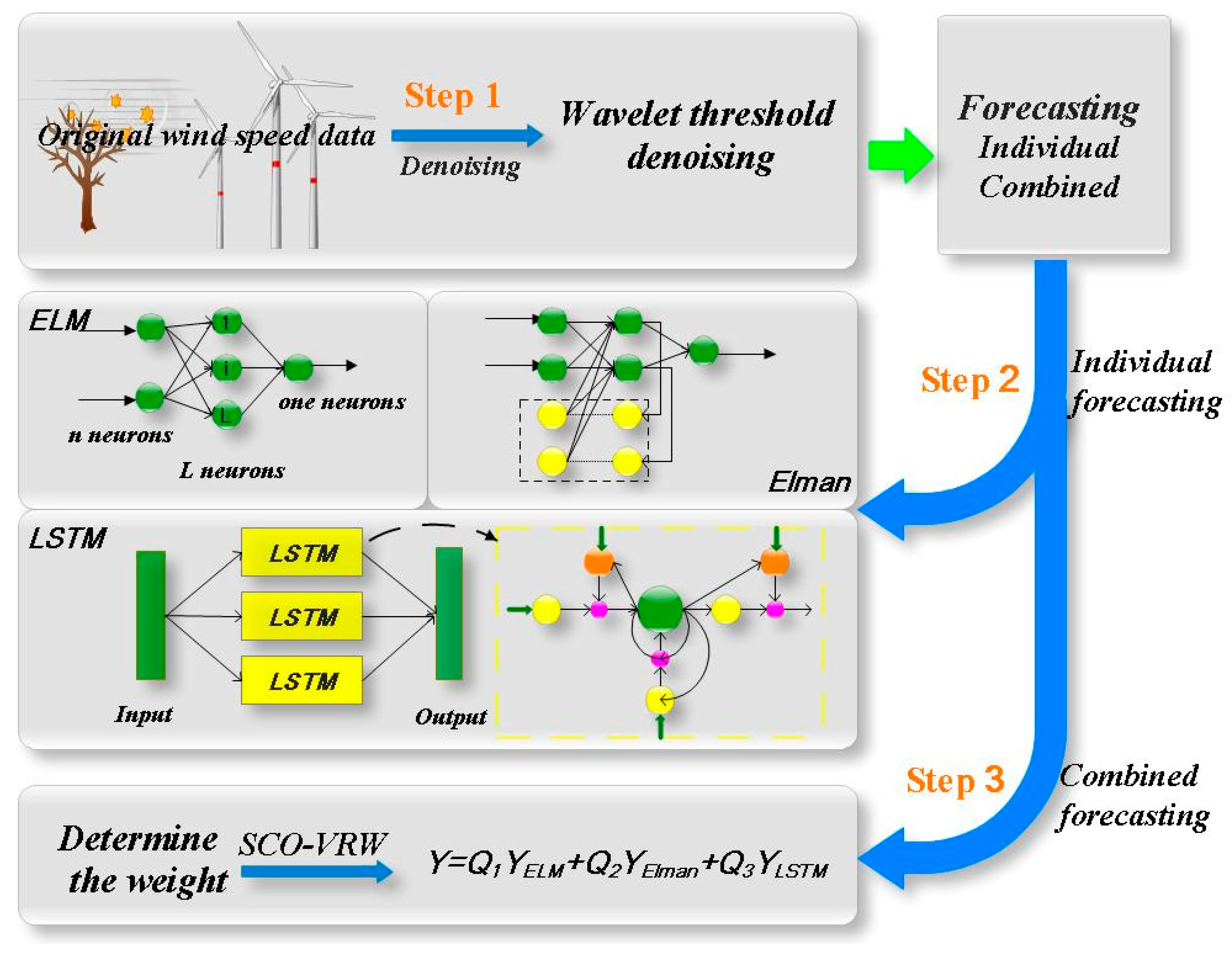
Wind speed at different heights is of great importance for a wind energy assessment of wind farms and the design of wind-resistance coefficients for high-rise buildings. In this paper, the combined forecasting model ELM–Elman–LSTM based on the SCO algorithm is proposed for wind speed forecasting at different heights. Firstly, the original wind speed data is de-noised by the wavelet threshold algorithm, and then the data are put into the model for calculation. The calculation results of each model are combined with the variance reciprocal method to obtain the intermediate forecasting results. Finally, we use the SCO algorithm to optimize the weight coefficient to obtain the final forecasting result. The social cognitive optimization algorithm is an optimization algorithm based on the core of the social cognitive theory. We will introduce it in detail in later sectionsections. In order to test the forecasting performance of the combined model and the forecasting accuracy at different heights, this paper selects the wind speed data at the heights of 20 m, 50 m, and 80 m at the National Wind Technology Center M2 Tower. Experimental results show that the combined model ELM–Elman–LSTM can improve the forecasting accuracy and provide good forecasting results for wind speed data at different heights.
The structure of this paper is as follows. The Section 1 mainly introduces the background, the significance, and several methods of wind speed forecasting, such as artificial neural network, combined forecasting, and hybrid forecasting. The Section 2 introduces the theoretical knowledge of artificial neural networks involved in the combination model proposed in this paper. The Section 3 proposes the combination model and the evaluation index of the model selected in this paper. The Section 4 introduces the experimental data and dataset division. In the Section 5, we experiment and analyze the results of experiments. In order to illustrate the forecasting performance of the combined model, the combined model is compared to three single models. In the Section 6, we summarize the experiment.
2. Materials and Methods
There are diverse ANNs for wind speed forecasting, such as the BP neural network, the Radical Basis Function (RBF) neural network, and the Generalized Regression Neural Network (GRNN). Every artificial neural network has a certain superiority as well as limitations for wind speed forecasting. In this paper, we choose three different artificial neural networks: the extreme learning machine (ELM), the Elman neural network, and Long Short-term Memory (LSTM) networks.
2.1. Extreme Learning Machines
The extreme learning machine [25,26], proposed by Huang Bin, is a new type of fast-learning algorithm. The ELM has a faster learning speed not merely because it can obtain the output weights by randomly initializing the input weight and bias but because it can determine parameters without iteration when compared to traditional artificial neural networks, especially single hidden-layer feedforward neural networks (SLFNs) [25]. The basic network architecture of the ELM has the input layer, the hidden layer, and the output layer. It is assumed that there are n neuron nodes in the input layer, neuron nodes in hidden layer, and only one neuron node in the output layer of the ELM. For samples , the operating principles of the ELM are as follows:
- a.
- The weight matrix (wi) from the input layer to the hidden layer and the bias (bi) of the hidden layer neuron are randomly set.
- b.
- The output matrix H of the hidden layer is calculated, and a wireless differentiable function (g(∗)) is selected as the hidden layer neuron activation function. The output matrix (H) is as follows:
- c.
- The weight () of the output layer is calculated. The final output of the network is as follows:
The cost function of the ELM is as follows:
The ultimate goal of the ELM is to obtain the smallest , which is as follows:
is the target value matrix of the sample set. According to the singular value decomposition [27] and Moore–Penrose generalized inverse [28,29], the weight matrix of the output layer is obtained.
2.2. Elman Neural Network
The Elman neural network, a recursive neural network with a local memory unit and a local feedback connection, was proposed by J. L. Elman. The structure of the Elman neural network mainly includes the input layer, correlation layer, hidden layer, and output layer. The correlation layer is a special hidden layer that receives feedback signals from the hidden layer. In the Elman neural network structure, there is full connectivity among the neuron nodes of the hidden layer and those of the correlation layer. The learning algorithms of the Elman neural network are as follows:
The connection weight between the hidden layer and the output layer is , the weight between the input layer and the correlation layer is , and the weight between the hidden layer and the output layer is . The input and output of each layer are as follows.
Input layer: The input layer only plays the role of signal transmission, so the input and output are all .
Correlation layer:
Input:
Output:
Hidden layer:
Input:
Output:
Output layer:
Input:
Output:
2.3. Long Short-Term Memory Neural Network
Hochreiter and Schmidhuber first proposed the long short-term memory (LSTM) neural network [30]. In follow-up work, it was improved and promoted by Alex Graves [31]. LSTM, a special kind of recurrent neural network (RNN), has achieved good performance in many fields, such as speech recognition, image recognition, and data forecasting. Unlike the traditional artificial neural network, the RNN introduces a directed loop in the network. That is to say, there is a full connection between the hidden layer and the hidden layer, which enables the RNN to effectively deal with the related problems. The structure of the RNN contains an input layer, a hidden layer, and an output layer, and the training algorithm of the RNN is the Backpropagation through time (BPTT) algorithm. However, the BPTT algorithm cannot solve the problem of long-term dependence. Therefore, the objective of LSTM is to solve the long-term dependence.
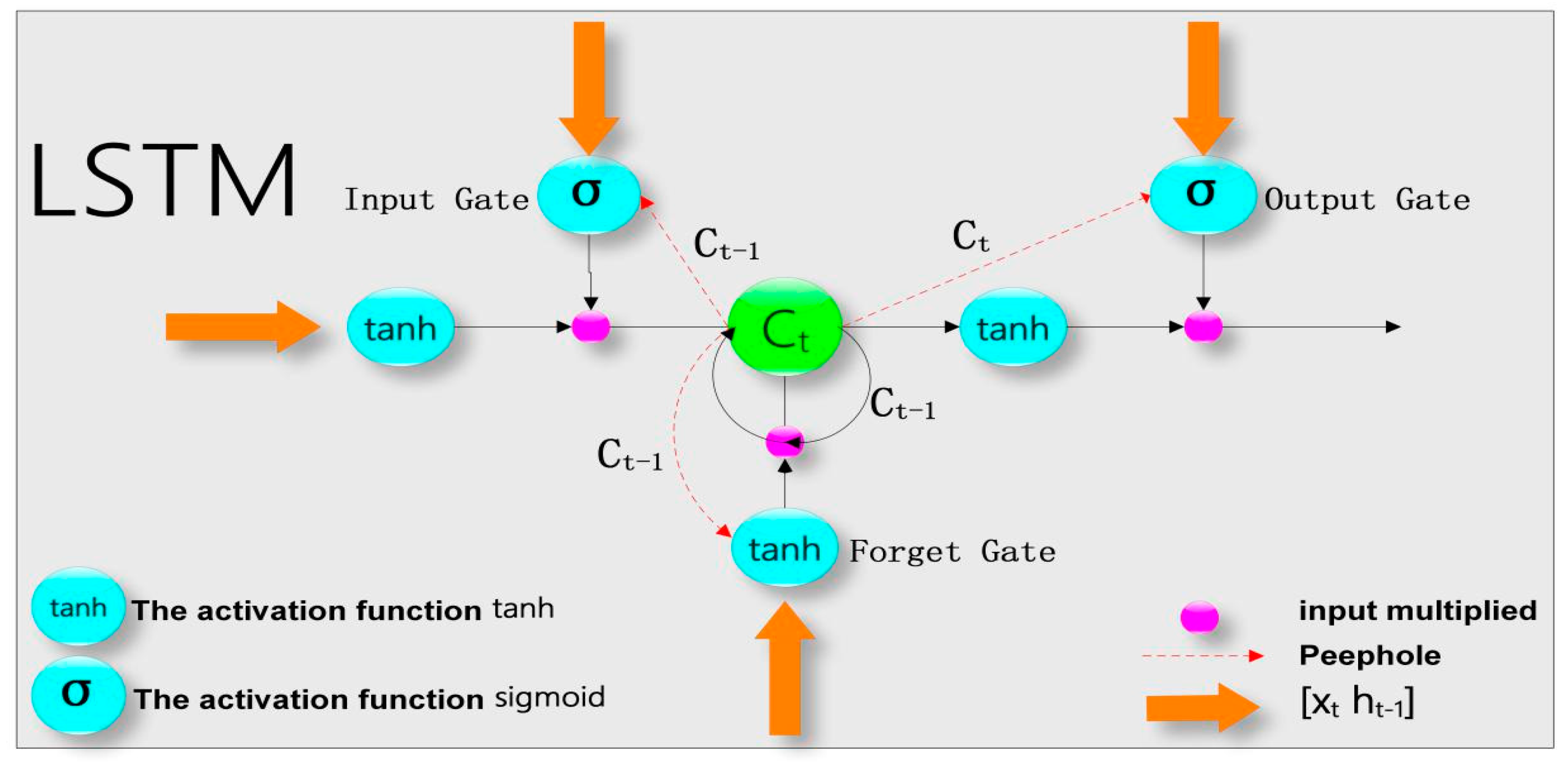
The structure of LSTM is shown in Figure 1 as a special kind of RNN. The difference between LSTM and other RNNs is that LSTM introduces a processor cell to judge whether the information is useful, and the core of LSTM is this cell. There are three gates in the cell: the input gate, the forget gate, and the output gate. The input gate determines how much the input of the network at the current moment can reach the cell. The output gate controls the output of the cell. The forget gate determines whether the output of the previous state is fully retained, partially retained, or completely forgotten in the current state. The training algorithm of LSTM also selects the BPTT algorithm. The learning steps of LSTM mainly include forward propagation and reverse propagation.

Figure 1.
The structure of the LSTM neural network.
Forward propagation:
Input gate:
Forget gate:
Cell:
Output gate:
The final output:
In the above formula, is the sigmoid function, and is hyperbolic function. The mathematical expressions are as follows:
Backpropagation is a process of error propagation that includes two directions: one is the reverse error in time, and the other is the reverse error in space. Additionally, back propagation is a process of updating the weight matrices and thresholds of the input gate, the output gate, the forgetting gate, and the cell. Because partial differential derivation is very complex in backpropagation, it is not described in detail in this paper, and detailed content can be found in the literature [32].
3. Proposed Combined Model
For the core of the combination model, there are many ways to determine the weight coefficients, such as the combination model with equal weights or unequal weights. In this paper, we choose the variance reciprocal method to calculate the weight of the combined model ELM–Elman–LSTM, and then optimizes the weight coefficients using the social cognitive optimization (SCO) algorithm.
3.1. SCO-VRW
In this paper, we use the SCO-VRW method to calculate the weight coefficient of the combined model. That is to say, we first use variance reciprocal weighting (VRW) to determine the weight coefficients of the combined model, and then we use the SCO algorithm to optimize the weight coefficients. Variance reciprocal weighting is a more commonly used method for determining the weight coefficient. A model with a smaller sum of square error was given a high weight. On the contrary, a model with a higher sum of square error was given a lower weight. The calculation method is as follows:
where represents the weight of the ith method, and and represent the forecasted value and target value of the ith method at time , respectively.
At present, there are many bionic intelligent optimization algorithms used to optimize the weight coefficient. The bionic intelligent optimization algorithm is an efficient approximation algorithm, similar to the ant colony optimization (ACO), particle swarm optimization (PSO), and cuckoo search (CS) algorithms. Most of these algorithms are based on insect society. Some authors [33] have proposed a social cognitive optimization (SCO) algorithm based on social cognitive theory. The SCO algorithm simulates social learning ability in social cognitive theory through competitive selection and domain search. In the specific implementation of the algorithm, agents are used to represent people in society. Knowledge in society is expressed by the knowledge base. Furthermore, the social learning process is simulated through the interaction between agents and the knowledge library to achieve optimization. There are four significant concepts for the SCO algorithm:
- (a)
- Knowledge point: A knowledge point is composed of position x and its horizontal description.
- (b)
- Library: A base is a table that contains the knowledge points.
- (c)
- Social cognitive agent: A social cognitive agent is a behavioral individual that dominates the knowledge point in the base; additionally, it contains a memory and a set of action rules.
- (d)
- Neighborhood search: It is assumed that there are two knowledge points, which are x1 and x2; the neighborhood search of x1 uses x1 as the reference point and x2 as the center point to calculate a new knowledge point variable, x3:
Assuming that the number of knowledge points in the library is , the number of social cognitive agents is , and the iterative frequency is . The flow chart of the SCO algorithm is shown in Figure 2. According to Figure 2, the basic steps of the SCO algorithm are as follows:
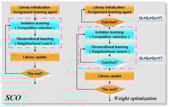
Figure 2.
The flowchart of the SCO algorithm and the weight optimization.
- (1)
- Initialization. The Npop knowledge points are randomly initialized, and the knowledge points in the library are randomly assigned to each social cognitive agent. However, assigning a knowledge point to multiple social cognitive agents repeatedly is prohibited.
- (2)
- Alternative learning process. The following actions are performed for each social cognitive agent.
- Imitation selection. First, two or more points (the selected knowledge points differ from the current social cognitive agent) are randomly selected from the library. Then the fitness values of the selected knowledge points are compared, and the best one is chosen based on the principle of competitive selection.
- Observational learning. First, the fitness value of the knowledge point selected through imitation selection is compared to that of the social cognitive agent. The best point is taken as the central point and another point as the reference point. The social cognitive agent is updated based on the neighborhood searching principle, and the new knowledge point is saved to the base.
- (3)
- Updates to the library. There are Nc new knowledge points increased in the process of alternative learning. Nc knowledge points with the worst fitness need to be removed from the library in order for the number of knowledge points in the library to remain unchanged.
- (4)
- Whether the result satisfies the end conditions must be determined. If it does not, step (2) to step (4) must be repeated until the end condition is reached.
Figure 2 shows the flowchart of weight coefficient optimization, and the following points should be paid attention in the process of optimization.
- In the initialization process of the library, the knowledge points in the library should meet the precondition that the sum of the weight coefficients is 1. Otherwise, it must be reinitialized.
- There will be a new knowledge point in the observational learning process, and new knowledge points need to be tested to meet the precondition that the sum of the weight coefficient is 1.
3.2. ELM–Elman–LSTM Model
The structure diagram of the combined ELM–Elman–LSTM model is shown in Figure 3. According to Figure 3, the basic forecasting steps using the ELM–Elman–LSTM model are as follows.

Figure 3.
The structure diagram of ELM–Elman–LSTM model.
Step 1: Data de-noising. The wavelet threshold algorithm is used to de-noise the original wind speed data.
Step 2: Three single models are used individually to forecast the data after noise reduction.
- Using the ELM neural network to train the wind speed data after the noise reduction and obtain the forecasting result y1.
- Using the Elman neural network to train the wind speed data after the noise reduction and obtain the forecasting result y2.
- Using the LSTM neural network to train the wind speed data after the noise reduction and obtain the forecasting result y3.
Step 3: Forecasting the wind speed data with the ELM-Elman-LSTM model.
- Using the variance reciprocal weighting method to calculate the weight of the combined model.
- Using the SCO algorithm to optimize weight. The final forecasting results are as follows.
3.3. Evaluation Index
Generally, the evaluation indices used commonly are the MAE, MSE, RMSE, MAPE, and SSE. Each evaluation index has its advantages and limitations, so it cannot evaluate the model’s forecasting performance from one angle. This paper chooses the MAE, MSE, MAPE, and R-squared values as the evaluation indices to evaluate the proposed model ELM–Elman–LSTM; the mathematical expressions are as follows. The smaller the values of the MAE, MSE, and MAPE, the better the forecasting results. While R-squared represents a fitting effect through the change of data, and the range of value is between (0, 1), the closer to 1, the better the fitting effect of the model.
4. Dataset Information
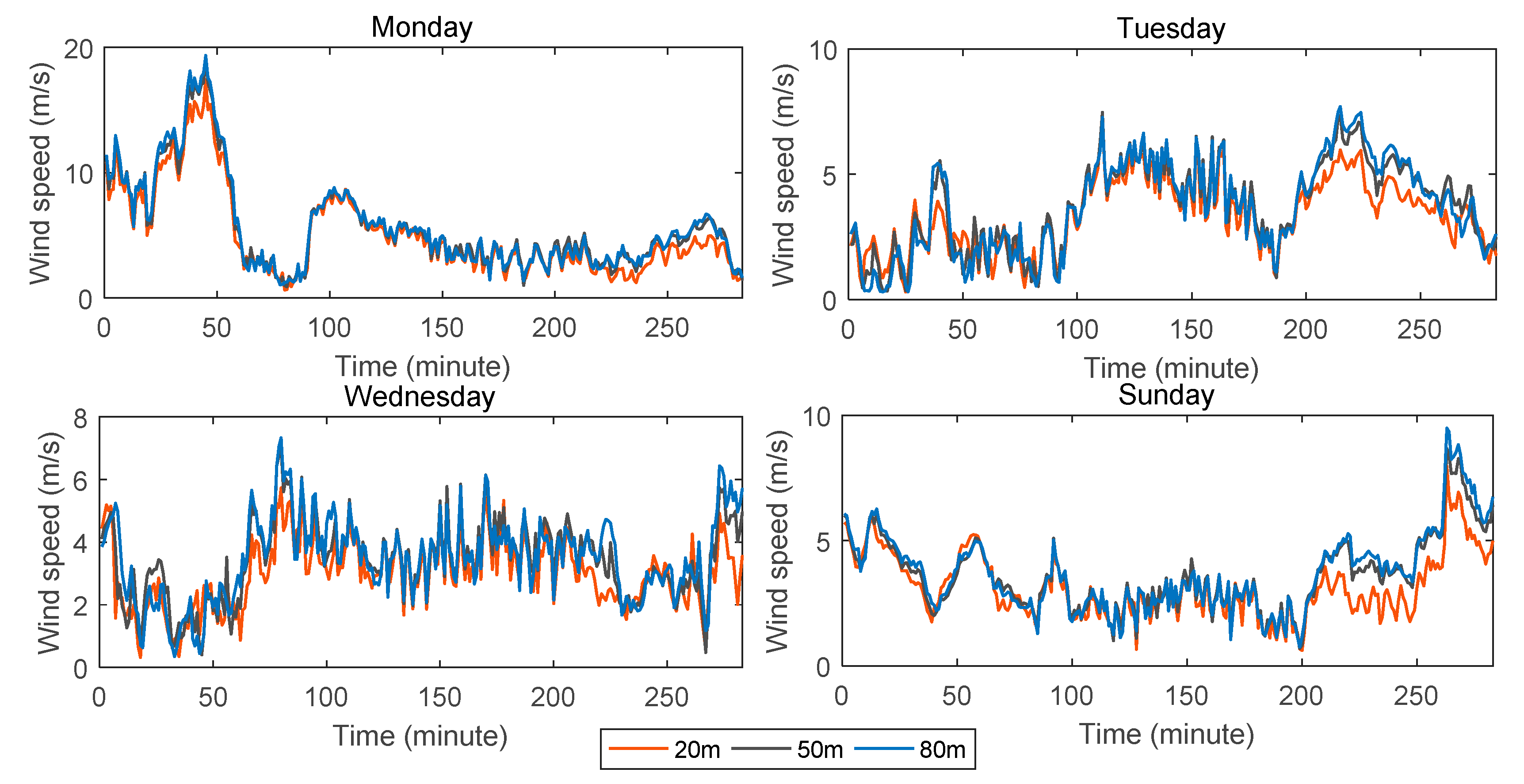
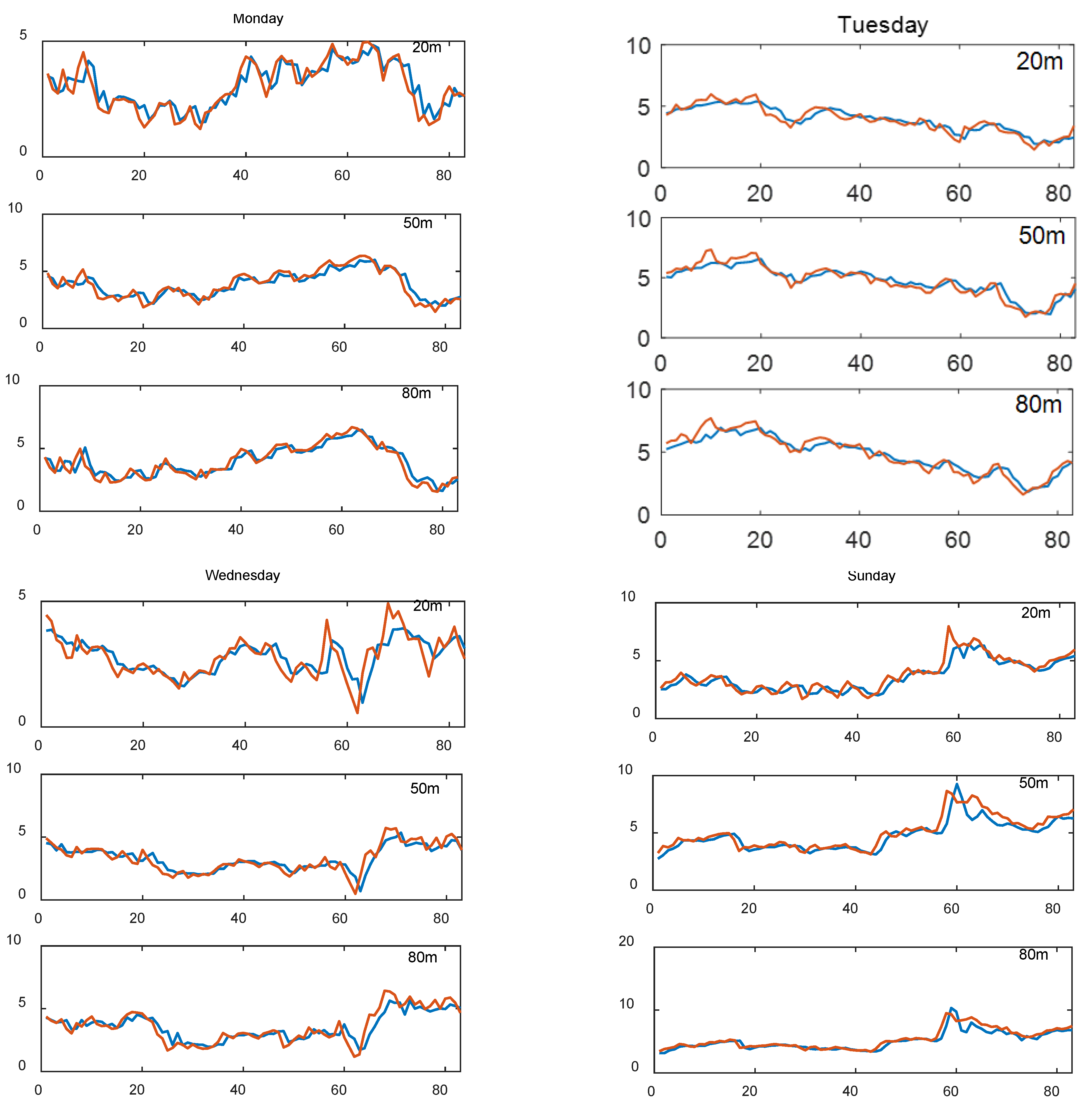
In order to test the forecasting performance of the proposed model in this paper and the effect of wind speed forecasting at different heights, we selected wind speed data at the National Wind Technology Center M2 Tower. The data are from 10 April to 12 April and 16 April 2017 as experimental data, and they are from Monday, Tuesday, Wednesday, and Sunday. The experimental data include three heights: wind speed data at heights of 20 m, 50 m, and 80 m. The data were sampled every five minutes and collected from 0:00 to 23:59, so there were 288 observations per day. The wind speed data of each height are shown in Figure 4. As can be seen from the figure, the general trend of wind speed data at each height is the same, and the higher the height, the greater the wind speed. In addition, comparing the four maps in the figure, we can see that the wind speed data selected in this paper are not periodic, and the wind speed data vary from one day to another.
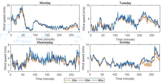
Figure 4.
Observations of wind speed at different heights.
When wind speed data are measured and collected, noise is generated for various reasons. The original wind speed data will be noise-reduced to improve the forecasting accuracy. The noise reduction methods used commonly are EMD, EEMD, and PCA. In this paper, we choose the wavelet threshold method for data de-noising. We use soft threshold de-noising and hard threshold de-noising to process the same set of data. A better method with an excellent de-noising effect is selected. Generally speaking, the effect of de-noising is evaluated by SNR and mean square error (MSE). The higher the SNR, the better the de-noising effect, and the smaller the MSE, the better the effect. The results of the noise reduction are shown in Table 1. It can be seen from the table that the effect of hard threshold de-noising is better than that of soft threshold de-noising.

Table 1.
The results of hard threshold and soft threshold de-noising.
Figure 5 shows the input and output of the ELM–Elman–LSSVM model. The data at the three heights have the same input and output modes: for example, at 20 m high, using data from times 1 to 5 to forecast the wind speed data at time 6 and using data from times 2 to 6 to forecast the wind speed data at time 7. In this way, the wind speed data of times K to K + 4 are used to forecast the wind speed data at time K + 5. Therefore, the input of the model is the wind speed data at time K to time K + 4, and the output is the wind speed data at time K + 5. The input vector has a dimension of 5, and the output vector has a dimension of 1. In other words, for the artificial neural network selected in this paper, the number of nodes in the input layer is 5, and the number of nodes in the output layer is 1.
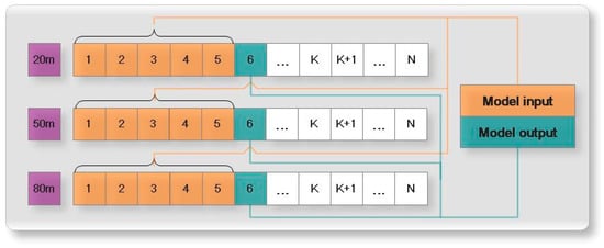
Figure 5.
The input and output of the ELM–Elman–LSTM model.
5. Experiment Results
In order to better illustrate the forecasting performance of the combined forecasting model ELM–Elman–LSTM, we compare the forecasting results of the combined model with that of the three single models (ELM, Elman, and LSTM) from the four evaluation indices (MSE, MAE, MAPE, and R-squared).
5.1. Forecasting Results of Individual Models
In forecasting with single models, the evaluation indices for the model we selected are the MAE, MSE, and MAPE. The number of hidden layers and neurons in each hidden layer greatly impacts the forecasting results. For the ELM network, there is only one hidden layer. For the data selected in this paper, compared to the 20 hidden layer neurons network, the forecasting effect is better than that of the ELM network of 10 hidden layer neurons. The forecasting results of ELM network are shown in Figure 6. Table 2 shows the evaluation indices of the ELM network.
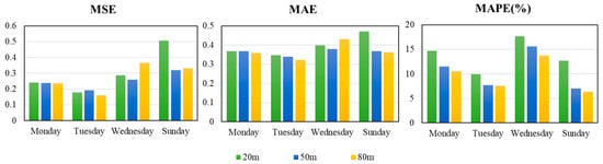
Figure 6.
The bar chart for the evaluation index of the ELM network.
Table 2.
The evaluation index of the ELM network.
First, by comparing the forecasting results of different datasets at the same height, we can obtain the following results. For wind speed data at the height of 20 m, the ELM network had the best forecasting effect on Tuesday with the minimum values of three evaluation indices: the value of the MSE was 0.1773, the value of the MAE was 0.3475, and the value of the MAPE was 9.89%. For wind speed data at the heights of 50 m and 80 m, there were the smallest values of the MSE and MAE on Tuesday, while the smallest value of the MAPE occurred on Sunday. For example, the value of the MSE was 0.1914, the value of the MAE was 0.3387, and the value of the MAPE was 7.03%.
Second, we compared the forecasting results at different heights within the same dataset. It can be seen that the value of the MAPE decreases gradually as the height increases for all datasets. However, the changes were not regular. For example, in the forecasting results on Tuesday, the MAPE values were 9.89%, 7.68%, and 7.51% at the heights of 20, 50, and 80 m, respectively. There is no particular relationship between height and the values of the MSE and MAE. For example, in the forecasting results on Tuesday, the MSE and MAE values were 0.1773 and 0.3475, respectively, at the height of 20 m. The MSE and MAE values were 0.1914 and 0.3387, respectively, at the height of 50 m. At the same time, the MSE and MAE values were 0.1603 and 0.3222, respectively, at the height of 80 m.
In addition, the forecasting results at the height of 80 m on Sunday were the best, wherein the MAPE was 6.34%.
When using the Elman neural network to forecast the wind speed, the same attention should be paid to the selection of hidden layer nodes. The results are shown in Figure 7. Table 3 shows the evaluation index of Elman.
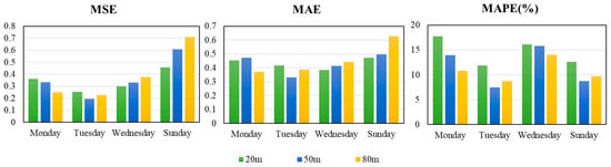
Figure 7.
The bar chart for the evaluation index of the Elman neural network.
Table 3.
The evaluation index of Elman.
First, by comparing the forecasting results of the data at the same height of different datasets, we can obtain the following results. For wind speed data at the height of 20 m, the forecasting results of the Elman neural network had the smallest values of the MSE and MAPE on Tuesday. The value of the MSE was 0.2540 and of the MAPE was 11.89%, while the value of the MAE was 0.4179, which is higher than that on Wednesday. For wind speed data at the height of 50 m, there were the smallest values of three evaluation indices on Tuesday. The value of the MSE was 0.1936, the MAE was 0.3315, and the MAPE was 7.46%. For wind speed data at the height of 80 m, there were the smallest value of the MSE and MAPE on Tuesday, while the value of the MAE was higher than that on Monday.
Second, by comparing the forecasting results of wind speed at different heights in the same dataset, we can see that there is no definite rule for the change of three evaluation indices. For example, on Monday, the values of the MSE and MAPE decreased as the height increased, while the value of the MAE did not have the same regular. On Wednesday and Sunday, the values of the MSE and MAE increased as the height decreased, but the change in the MAPE was not the same. In addition, on Monday and Wednesday, the value of the MAPE decreased as the height increased. In short, when using the Elman neural network for wind speed forecasting at different heights, it is not certain that the value of the MAPE will decrease as the height increases.
In addition, the forecasting results at the height of 50 m on Tuesday were the best, wherein the value of the MAPE was 7.46%.
The wind speed data after noise reduction were entered into the LSTM network, and the forecasting results are shown in Figure 8 and Table 4. According to the figure and table, we can make the following conclusions.
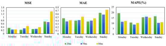
Figure 8.
The bar chart for the evaluation index of the LSTM network.
Table 4.
The three evaluation indices of the LSTM model.
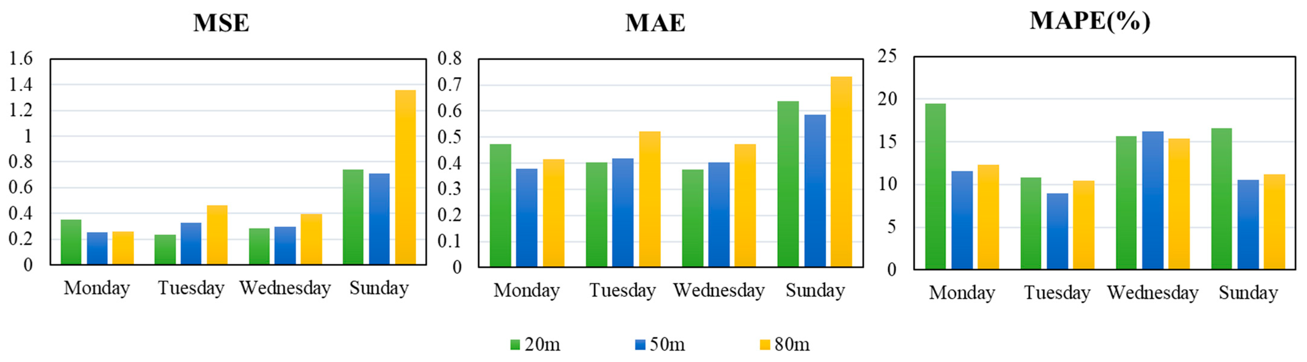
First of all, we compared the forecasting results at the same height of different datasets. It can be concluded that the LSTM network had a better forecasting performance at the height of 20 m on Tues day, while the value of the MAPE was 10.87% and of the MSE was 0.2336, the smallest value in all forecasting results. For heights of 50 m and 80 m, there were the smallest values of the MSE and MAE on Wednesday, but the value of the MAPE was relatively large at this time. For example, at the height of 50 m, the value of the MAPE was 16.26% on Wednesday, while the value of the MAPE was 8.94% on Tuesday.
Secondly, in comparing the forecasting results at different heights of the same dataset, it can be seen that the LSTM network does not have specific rules for wind speed forecasting at different heights from the three evaluation indices. However, from the perspective of the MAPE alone, among the four-day forecasting results, except for Wednesday, there were three days that the value of the MAPE was the smallest at the height of 50 m. This also shows that the LSTM network has some advantages for wind speed forecasting at the height of 50 m.
5.2. Forecasting Results of ELM–Elman–LSTM
The forecasting results of the ELM, Elman, and LSTM networks were combined with a certain weight using a variance reciprocal weighting method, and then the weight coefficient was optimized by the SCO algorithm. Figure 9 shows the forecasting results of the ELM–Elman–LSTM model. It can be seen from the figure that the forecasting curve of the combined model ELM–Elman–LSTM is basically in line with the actual price curve. Especially at the heights of 50 m and 80 m on Sunday, the forecasting curve is closer to the actual price curve. In comparison, the fit between the forecasting curve and the actual price curve at the height of 20 m is not as good as that of the remaining two heights.
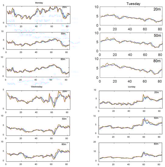
Figure 9.
The forecasting results of the ELM–Elman–LSTM model and the observation of wind speed.
In order to better prove the forecasting performance of the combined model, the ELM–Elman–LSTM model was compared to three single models (ELM, Elman, and LSTM). Table 5 records the three evaluation indices (MSE, MAE, and MAPE), and Table 6 records the value of R-squared of the four models.
Table 5.
The three evaluation indices value of the ELM–Elman–LSTM model and the single models.
Table 6.
R-squared of the ELM–Elman–LSTM model and the three single models.
First, we made a simple comparison of three individual models. The MAE and MSE of the ELM network were higher than those of the other two models at the height of 20 m on Wednesday, and the MAE and MSE of the ELM network were less than those of the other two models in the remaining datasets. The MAPE using the ELM network was higher than that of the Elman network at the height of 50 m on Wednesday and 20 m on Sunday. The MAPE of the ELM network was higher than those of the other two models at the height of 20 m on Wednesday. Except for these two cases, the three evaluation indices of the ELM network were smaller than those of the other two models. Based on this, it can also be said that the ELM network has better forecasting performance than the Elman and LSTM networks. In addition, it can also be seen from the table that the evaluation indices of the Elman and LSTM networks fluctuate up and down, and the two models have different advantages for different datasets. Next, we compared the combined model with single models.
We compared the forecasting results of the ELM–Elman–LSTM model with those of the ELM neural network. The value of the MSE using the ELM–Elman–LSTM was higher than that of the ELM network at the height of 50 m on Wednesday and Monday. For example, for the wind speed at the height of 50 m on Wednesday, the MSE was 0.2600 for the ELM–Elman–LSTM model, while the MSE of the ELM network was 0.2587. Except for the above case, the values of the three evaluation indices of the remaining datasets were less than those of the ELM network. For example, for the wind speed data at the height of 20 m on Monday, the MAPE of the ELM network is 14.68%, and the MAPE of the ELM–Elman–LSTM model is 13.46%, a decrease of 1.22%.
We compared the forecasting results of the ELM–Elman–LSTM model with those of the Elman neural network. The value of the three evaluation indices forecasted by the ELM–Elman–LSTM model was smaller than that of the Elman network. It can also be said that the forecasting performance of the ELM–Elman–LSTM model is better than that of Elman neural network. For example, for the weed speed data forecasted by the Elman neural network at the height of 20 m on Tuesday, the MSE was 0.2540, the MAE was 0.4179, and the MAPE was 11.89%. On the other hand, the MSE was 0.1618, the MAE was 0.3140, and the MAPE was 8.63%, forecasted by the ELM–Elman–LSTM model, a value decrease of 3.26%.
We compared the forecasting results of the ELM–Elman–LSTM model with those of the LSTM neural network. The value of the three evaluation indices forecasted by the ELM–Elman–LSTM model was smaller than that of the LSTM network for all datasets, as observed from the angle of the MAPE. It can be seen that the value of the MAPE is greatly reduced when forecasted by the ELM–Elman–LSTM model. For example, at the height of 80 m on Sunday, the MAPE of the LSTM network was 11.69%, whereas the MAPE of the ELM–Elman–LSTM model was 5.96%, a decrease of 5.73%.
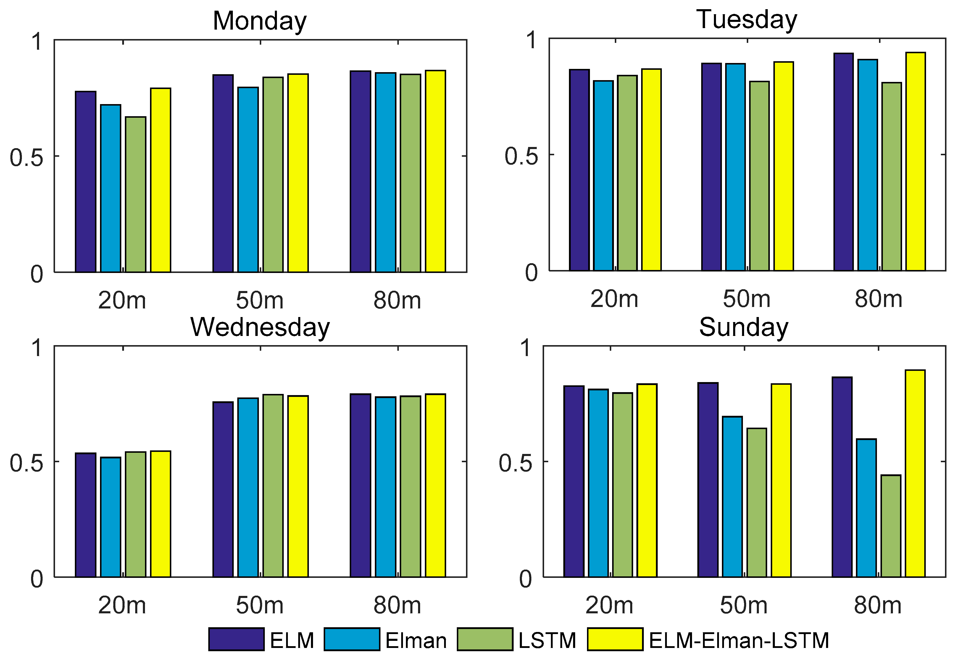
In conclusion, when using the MSE, MAE, and MAPE to evaluate the model, the forecasting performance of the ELM–Elman–LSTM model for forecasting wind speed at different heights is superior to the three single forecasting models. According to Table 6 and Figure 10, for the wind speed at the height of 50 m on Sunday, the R-squared value forecasted by the ELM–Elman–LSTM model is smaller than that of the ELM network. For the remaining datasets, the R-squared value of the ELM–Elman–LSTM model is greater than those of the other three individual models. Moreover, the R-squared value of the combined model ELM–Elman–LSTM is close to 1. For example, for the data at the height of 80 m on Tuesday, the R-squared value of the ELM–Elman–LSTM reached 0.9388, but for the data at the height of 20 m on Wednesday, the value of R-squared of the four methods was not very close to 1; the highest value was 0.5447.

Figure 10.
The value of R-squared for the four models.
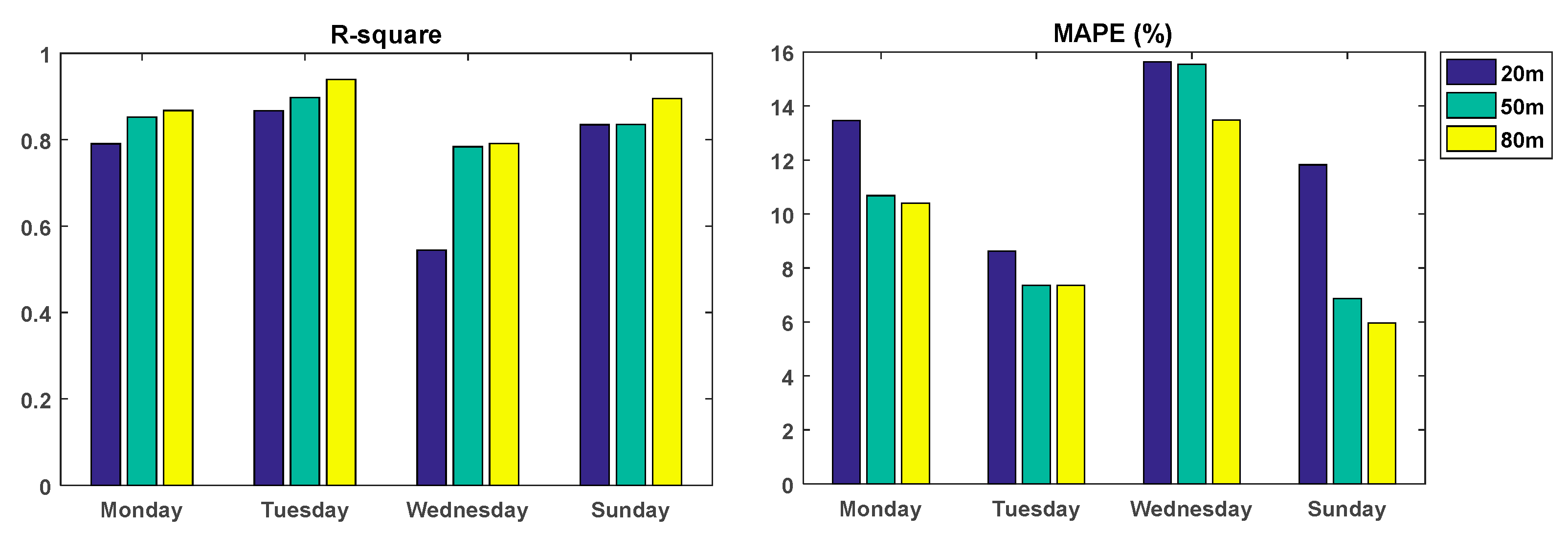
Next, we compare the forecasting result of the ELM-Elman-LSTM model on wind speed data at different heights. Figure 11 shows the value of the R-squared coefficient and MAPE of the combined model ELM-Elman-LSTM at different heights. According to Figure 11 and Table 6, we can see that the value of the R-squared of the wind speed data at the height of 80 m is maximum in the three heights and is also closest to 1. For example, the maximum value of R-squared can reach 0.9388. The value of the MAPE at the height of 80 m is greater than that at 50 m only on Tuesday. It also can be said that ELM-Elman-LSTM has the best forecasting performance for the wind speed at the height of 80 m. In addition, if the model is only evaluated from the perspective of R-squared, only the value of R-squared for wind speed at the height of 20 m on Wednesday is smaller, which is only 0.5447. For the rest of the dataset, the forecasting performance of the wind speed at the height of 20 m is as good as that at the height of 50 m. However, if we evaluate the model from the perspective of the MAPE, the forecasting performance of the data at the height of 50 m is better than that at 20 m.
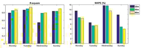
Figure 11.
The value of R-squared and MAPE for the combined model ELM–Elman–LSTM.
In short, it can be seen from the forecasting results that the ELM–Elman–LSTM model can improve forecasting accuracy compared to a single forecasting model and can obtain better forecasting results for wind speed data at different heights. Significantly, the forecasting result at the height of 80 m was perfect.
5.3. Improvements of the Proposed Combined Model
An MAPE improvement criterion is applied in this subsection, which calculates the improvement of the MAPE by using the MAPE of the proposed combined model and the MAPE of the other models. It is defined as:
To prove that the presented combined model indeed improves the wind speed forecasting accuracy, the MAPE values of the ELM–Elman–LSTM model are compared to the MAPE values of the ELM, Elman, and LSTM models. Table 7 lists the results of for the model that has been proposed and for the other forecasting models. From Table 7, when compared to three individual models, the ELM–Elman–LSTM model exhibits huge enhancements for multi-step forecasting. In particular, for Sunday at 80 m, the presented method average leads to 5.99%, 38.49%, and 46.74% reductions, respectively, in comparison with the ELM, Elman, and LSTM models.
Table 7.
Improvement percentages of the ELM–Elman–LSTM model.
6. Conclusions
As a kind of renewable green energy, wind energy utilization has become an increasingly important concern. Using wind power to replace traditional energy combustion power generation is an essential application method that can reduce the pressure caused by the gradual reduction in traditional energy sources, reduce environmental pollution, and contribute to the sustainable development of society. Therefore, how to effectively and reasonably apply wind energy has become the focus of much research. Wind speed is a direct manifestation of wind energy, and accurate wind speed forecasting has a significant impact on the allocation of wind farms and the stable development of the electricity market. This paper proposes the combined forecasting model ELM–Elman–LSTM, and the social cognitive optimization (SCO) algorithm was used for the optimization of weight coefficients. In addition, in order to obtain better forecasting results, the original wind speed data were de-noised through the wavelet threshold method. The wind speed data at three different heights were chosen to test the model. The experimental results show that the ELM–Elman–LSTM model can improve forecasting accuracy compared to a single forecasting model. Furthermore, the ELM–Elman–LSTM has a better forecasting performance for wind speed at different heights.
Author Contributions
Conceptualization, Z.H. and J.X.; Methodology, Y.C.; Software, Z.H.; Validation, J.X. and Y.C.; Formal Analysis, Z.H. and J.X.; Investigation, J.X.; Resources, Y.C.; Data Curation, Z.H.; Writing—Review and Editing, Z.H. and Y.C.; Visualization, J.X. and Y.C.; Supervision, Y.C.; Funding Acquisition, J.X. All authors have read and agreed to the published version of the manuscript.
Funding
Supported by [National Natural Science Foundation of China] Grant Number [62071380].
Institutional Review Board Statement
Not applicable.
Informed Consent Statement
Not applicable.
Data Availability Statement
The data presented in this study are available on request from the corresponding author.
Conflicts of Interest
The authors declare that there are no conflicts of interest regarding the publication of this paper.
References
- Global Status of Wind Power. Available online: http://gwec.net/global-figures/wind-energy-global-status/# (accessed on 22 March 2022).
- Jahangir, H.; Golkar, M.A.; Alhameli, F.; Mazouz, A.; Ahmadian, A.; Elkamel, A. Short-term wind speed forecasting framework based on stacked denoising auto-encoders with rough ANN. Sustain. Energy Technol. Assess. 2020, 38, 100601. [Google Scholar] [CrossRef]
- Shukur, O.B.; Lee, M.H. Daily wind speed forecasting through hybrid KF-ANN model based on ARIMA. Renew. Energy 2015, 76, 637–647. [Google Scholar] [CrossRef]
- Liu, M.; Cao, Z.; Zhang, J.; Wang, L.; Huang, C.; Luo, X. Short-term wind speed forecasting based on the Jaya-SVM model. Int. J. Electr. Power Energy Syst. 2020, 121, 106056. [Google Scholar] [CrossRef]
- Santamaría-Bonfil, G.; Reyes-Ballesteros, A.; Gershenson, C. Wind speed forecasting for wind farms: A method based on support vector regression. Renew. Energy 2016, 85, 790–809. [Google Scholar] [CrossRef]
- Deveci, M.; Özcan, E.; John, R.; Covrig, C.-F.; Pamucar, D. A study on offshore wind farm siting criteria using a novel interval-valued fuzzy-rough based Delphi method. J. Environ. Manag. 2020, 270, 110916. [Google Scholar] [CrossRef]
- Cadenas, E.; Jaramillo, O.A.; Rivera, W. Analysis and forecasting of wind velocity in chetumal, quintana roo, using the single exponential smoothing method. Renew. Energy 2010, 35, 925–930. [Google Scholar] [CrossRef]
- Zhang, K.; Qu, Z.; Dong, Y.; Lu, H.; Leng, W.; Wang, J.; Zhang, W. Research on a combined model based on linear and nonlinear features-A case study of wind speed forecasting. Renew. Energy 2019, 130, 814–830. [Google Scholar] [CrossRef]
- Suyono, H.; Prabawanti, D.O.; Shidiq, M.; Hasanah, R.N.; Wibawa, U.; Hasibuan, A. Forecasting of Wind Speed in Malang City of Indonesia using Adaptive Neuro-Fuzzy Inference System and Autoregressive Integrated Moving Average Methods. In Proceedings of the 2020 International Conference on Technology and Policy in Energy and Electric Power (ICT-PEP), IEEE, Bandung, Indonesia, 23–24 September 2020; pp. 131–136. [Google Scholar]
- Moreno, S.R.; Dos Santos Coelho, L. Wind speed forecasting approach based on singular spectrum analysis and adaptive neuro fuzzy inference system. Renew. Energy 2018, 126, 736–754. [Google Scholar] [CrossRef]
- Singh, S.N.; Mohapatra, A. Repeated wavelet transform based ARIMA model for very short-term wind speed forecasting. Renew. Energy 2019, 136, 758–768. [Google Scholar]
- Liu, M.D.; Ding, L.; Bai, Y.L. Application of hybrid model based on empirical mode decomposition, novel recurrent neural networks and the ARIMA to wind speed prediction. Energy Convers. Manag. 2021, 233, 113917. [Google Scholar] [CrossRef]
- Altan, A.; Karasu, S.; Zio, E. A new hybrid model for wind speed forecasting combining long short-term memory neural network, decomposition methods and grey wolf optimizer. Appl. Soft Comput. 2021, 100, 106996. [Google Scholar] [CrossRef]
- Zhang, Y.; Chen, B.; Pan, G.; Zhao, Y. A novel hybrid model based on VMD-WT and PCA-BP-RBF neural network for short-term wind speed forecasting. Energy Convers. Manag. 2019, 195, 180–197. [Google Scholar] [CrossRef]
- Catalão, J.P.S.; Pousinho, H.M.I.; Mendes, V.M.F. Short-term wind power forecasting in Portugal by neural networks and wavelet transform. Renew. Energy 2011, 36, 1245–1251. [Google Scholar] [CrossRef]
- Khelil, K.; Berrezzek, F.; Bouadjila, T. GA-based design of optimal discrete wavelet filters for efficient wind speed forecasting. Neural Comput. Appl. 2021, 33, 4373–4386. [Google Scholar] [CrossRef]
- He, Z.; Chen, Y.; Shang, Z.; Li, C.; Li, L.; Xu, M. A novel wind speed forecasting model based on moving window and multi-objective particle swarm optimization algorithm. Appl. Math. Model. 2019, 76, 717–740. [Google Scholar] [CrossRef]
- Li, H.; Wang, J.; Lu, H.; Guo, Z. Research and application of a combined model based on variable weight for short term wind speed forecasting. Renew. Energy 2018, 116, 669–684. [Google Scholar] [CrossRef]
- Zhang, W.; Qu, Z.; Zhang, K.; Mao, W.; Fan, X. A combined model based on CEEMDAN and modified flower pollination algorithm for wind speed forecasting. Energy Convers. Manag. 2017, 136, 439–451. [Google Scholar] [CrossRef]
- Liu, Z.; Jiang, P.; Zhang, L.; Niu, X. A combined forecasting model for time series: Application to short-term wind speed forecasting. Appl. Energy 2020, 259, 114137. [Google Scholar] [CrossRef]
- Chen, Y.; Zhang, S.; Zhang, W.; Peng, J.; Cai, Y. Multifactor spatio-temporal correlation model based on a combination of convolutional neural network and long short-term memory neural network for wind speed forecasting. Energy Convers. Manag. 2019, 185, 783–799. [Google Scholar] [CrossRef]
- Wang, H.; Han, S.; Liu, Y.; Yan, J.; Li, L. Sequence transfer correction algorithm for numerical weather prediction wind speed and its application in a wind power forecasting system. Appl. Energy 2019, 237, 1–10. [Google Scholar] [CrossRef]
- Wang, H.; Han, S.; Liu, Y.; Yan, J.; Li, L. Forecasting the high penetration of wind power on multiple scales using multi-to-multi mapping. IEEE Trans. Power Syst. 2017, 33, 3276–3284. [Google Scholar]
- Hoolohan, V.; Tomlin, A.S.; Cockerill, T. Improved near surface wind speed predictions using Gaussian process regression combined with numerical weather predictions and observed meteorological data. Renew. Energy 2018, 126, 1043–1054. [Google Scholar] [CrossRef]
- Ali, M.; Prasad, R. Significant wave height forecasting via an extreme learning machine model integrated with improved complete ensemble empirical mode decomposition. Renew. Sustain. Energy Rev. 2019, 104, 281–295. [Google Scholar] [CrossRef]
- Alaba, P.A.; Popoola, S.I.; Olatomiwa, L.; Akanle, M.B.; Ohunakin, O.S.; Adetiba, E.; Alex, O.D.; Atayero, A.A.A.; Wan Daud, W.M.A. Towards a more efficient and cost-sensitive extreme learning machine: A state-of-the-art review of recent trend. Neurocomputing 2019, 350, 70–90. [Google Scholar] [CrossRef]
- Chen, H.; Zhang, Q.; Luo, J.; Xu, Y.; Zhang, X. An enhanced bacterial foraging optimization and its application for training kernel extreme learning machine. Appl. Soft Comput. 2020, 86, 105884. [Google Scholar] [CrossRef]
- Chen, Y.; Kloft, M.; Yang, Y.; Li, L. Mixed kernel based extreme learning machine for electric load forecasting. Neurocomputing 2018, 312, 90–106. [Google Scholar] [CrossRef]
- Zhao, H.; Liu, H.; Xu, J.; Deng, W. Performance prediction using high-order differential mathematical morphology gradient spectrum entropy and extreme learning machine. IEEE Trans. Instrum. Meas. 2019, 69, 4165–4172. [Google Scholar] [CrossRef]
- Hochreiter, S.; Schmidhuber, J. LSTM can solve hard long time lag problems. Adv. Neural Inf. Process. Syst. 1997, 9, 473–479. [Google Scholar]
- Graves, A.; Schmidhuber, J. Framewise phoneme classification with bidirectional LSTM and other neural network architectures. Neural Netw. 2005, 18, 602–610. [Google Scholar] [CrossRef]
- Van Houdt, G.; Mosquera, C.; Nápoles, G. A review on the long short-term memory model. Artif. Intell. Rev. 2020, 53, 5929–5955. [Google Scholar] [CrossRef]
- Yao, Z.; Wu, S.; Wen, Y. Formation generation for multiple unmanned vehicles using multi-agent hybrid social cognitive optimization based on the internet of things. Sensors 2019, 19, 1600. [Google Scholar] [CrossRef] [PubMed] [Green Version]


Publisher’s Note: MDPI stays neutral with regard to jurisdictional claims in published maps and institutional affiliations. |
© 2022 by the authors. Licensee MDPI, Basel, Switzerland. This article is an open access article distributed under the terms and conditions of the Creative Commons Attribution (CC BY) license (https://creativecommons.org/licenses/by/4.0/).