Study on Calculation Method for Wellbore Pressure in Gas Wells with Large Liquid Production

Abstract

In order to solve the inaccuracy in the calculation of the wellbore pressure distribution caused by large liquid production in the Donghai gas field, the gas–liquid production conditions of the Donghai gas field were simulated with indoor experiments, and the flow patterns for different pipe diameters, different inclinations, and different flow patterns were systematically analyzed using a flow pattern discrimination method, liquid holdup calculation method, and pressure drop calculation method. Using the experimental data, the division methods for different flow patterns were screened. Finally, based on the fact that the change trend for the flow patterns was consistent, the Kaya–Sarica–Brill method was selected to establish the flow pattern discrimination formula. According to the calculation method for the Mukherjee and Brill (M–B) liquid holdup, the M–B model was re-established according to a 75 mm pipe diameter and 60 mm pipe diameter using the instantaneous liquid holdup measured in the laboratory. Through the comparison and analysis of the measured data and the calculated data for the Beggs and Brill (B–B_ pressure drop model under the same working conditions, it was found that when the B–B model was applied to different angles and different gas–liquid ratios, the error decreased with an increase in the angle and increased with a decrease in the gas–liquid ratio. After verifying the correlation of different dimensionless numbers that can characterize the gas–liquid ratio, it was considered that the introduction of the Reynolds number into the original model could greatly improve the accuracy of the calculation, so a new pressure drop calculation model was established. The new pressure drop calculation model takes into account the two parameters of the well deviation angle and gas–liquid ratio. The accuracy was greatly improved, as verified by field measurements in four wells.

1. Introduction

With the substantial increase in the proportion of natural gas exploitation, the monitoring of gas wells is becoming ever more important. The correct calculation of the gas wellbore pressure distribution is related to the optimization of the completion string, the optimization of gas–well production parameters, the judgment of the amount of fluid accumulation in the gas well, and the prediction of the height of the fluid accumulation. After much research in China and other countries, a variety of gas–liquid two-phase flow and pressure drop calculation models have been established for the calculation of the wellbore pressure distribution.

There are six pressure drop calculation models commonly used for two-phase pipe flows, namely, the Aziz, Govier, and Fogarasi model [1], Beggs and Brill model [2,3], Hasan model, Mukherjee and Brill model [4,5,6], Orkiszewski model [7], and pattern model (a model formulated by Ruiquan Liao) [8]. The characteristics of each model are presented below.

Based on an experiment, the Aziz–Govier–Fogarasi model [1,9] puts forward a new discrimination method for bubbly flows and slug flows and recommends the Duns and Ros [10] discrimination method for annular flow and transition flow patterns. In the density and friction loss phase, the local gas-phase volume factor is introduced through the gas–liquid two-phase separation.

Beggs and Brill [2], and Chen [9] conducted indoor experiments on a gas–water two-phase mixture in a 15 m long pipeline with different inclination angles and obtained the correlation laws for the liquid holdup and resistance coefficient [2,9]. The relationship curves between the liquid holdup and inclination angle under different flow rates were drawn. A pressure drop calculation model of multiphase pipe flow considering arbitrary inclination angle is proposed for the first time. The model can be used in inclined and vertical pipes and has great applicability.

The Orkiszewski model evaluates and optimizes the pressure drop calculation method for gas–liquid two-phase flows with the data of 148 wells [7,9]. On this basis, the discrimination method for two-phase flow patterns was re-established, the liquid-phase distribution coefficient was defined, the calculation methods for the mixture density and friction pressure gradient under different flow patterns were provided, and a new pressure drop calculation method was established. The Orkiszewski method uses a large number of field-measured data to optimize the common methods, but it integrates too many methods, resulting in too many correlation coefficients to be calculated, a large amount of calculation, and too many parameters.

The Kaya–Sarica–Brill method [11] is a comprehensive mechanical model formulated based on previous studies on gas–liquid two-phase pipe flows in deviated wells. The model adopts five flow patterns of gas–liquid two-phase flows in vertical pipes established by Taitel [12] et al. and integrates Kaya–Sarica–Brill bubble flow transition model, Barnea’s dispersed bubble flow transition model, Tengesdal’s agitated flow transition model, and Ansari’s annular flow transition model. Using 2052 sets of data in the TUFFP database for error analysis, it is believed that, compared with the Hagedorn–Brown model, Chokshi model, Tengesdal model, Aziz–Govier–Fogarasi model, Hasan model, and Anssri model, the Kaya–Sarica–Brill model has the highest accuracy when applied to the TUFFP database.

The Mukherjee and Brill model was obtained after improving the experimental conditions based on the Beggs and Brill model [13,14]. An experiment was carried out in the range of pipeline inclination angles of 0°~90°, and the empirical formulae for the liquid holdup and friction coefficient were obtained through the regression of experimental data. The formula is more suitable for the calculation of the pressure gradients of inclined wells, directional wells, and horizontal wells.

The pattern method [8] is a comprehensive mechanism model obtained by Liao Ruiquan’s team by analyzing the international achievements in multiphase flow pattern divisions and pressure drop calculations and based on the research results of Hasan, Aziz, Banea [15], Titel, Duckler [16], and others. The values of some coefficients were determined through the repeated comparison and verification of indoor experimental data within the allowable range of the theory. This method has been used in many oil and gas fields in China for many years.

When using different methods to solve field practical problems, the commonly used empirical and semiempirical models have poor adaptability and great regionality, while the mechanism model has the problems of unclosed flow pattern prediction boundaries and incomplete flow pattern coverage. In 2013, Zhang Tingting et al. compared the calculated values for the model with the simulation results from the CFD software and considered that the gas–liquid ratio and pipeline inclination would affect the calculation accuracy of some models [17]. However, using the CFD software to verify the accuracy of the mathematical model is not rigorous. It is necessary to verify whether the views of Zhang Tingting and others are correct according to the physical model experimental data and correct the appropriate model on this basis. Chen Dechun evaluated eight common models by sorting pressure measurement data in China and other countries in 2017 [18]. He found that the same model error fluctuated under different gas–liquid ratios, which also confirmed that the applicable conditions for different models have certain limitations. According to the pressure drop optimization idea of Liao’s team and Mukherjee and Brill, a matched indoor experiment was established, the flow pattern and pressure drop calculation methods of predecessors were selected and optimized, and a new high-precision pressure drop calculation method was established according to the production conditions of the Donghai gas field.

2. Experimental Phenomena and Flow Pattern Discrimination

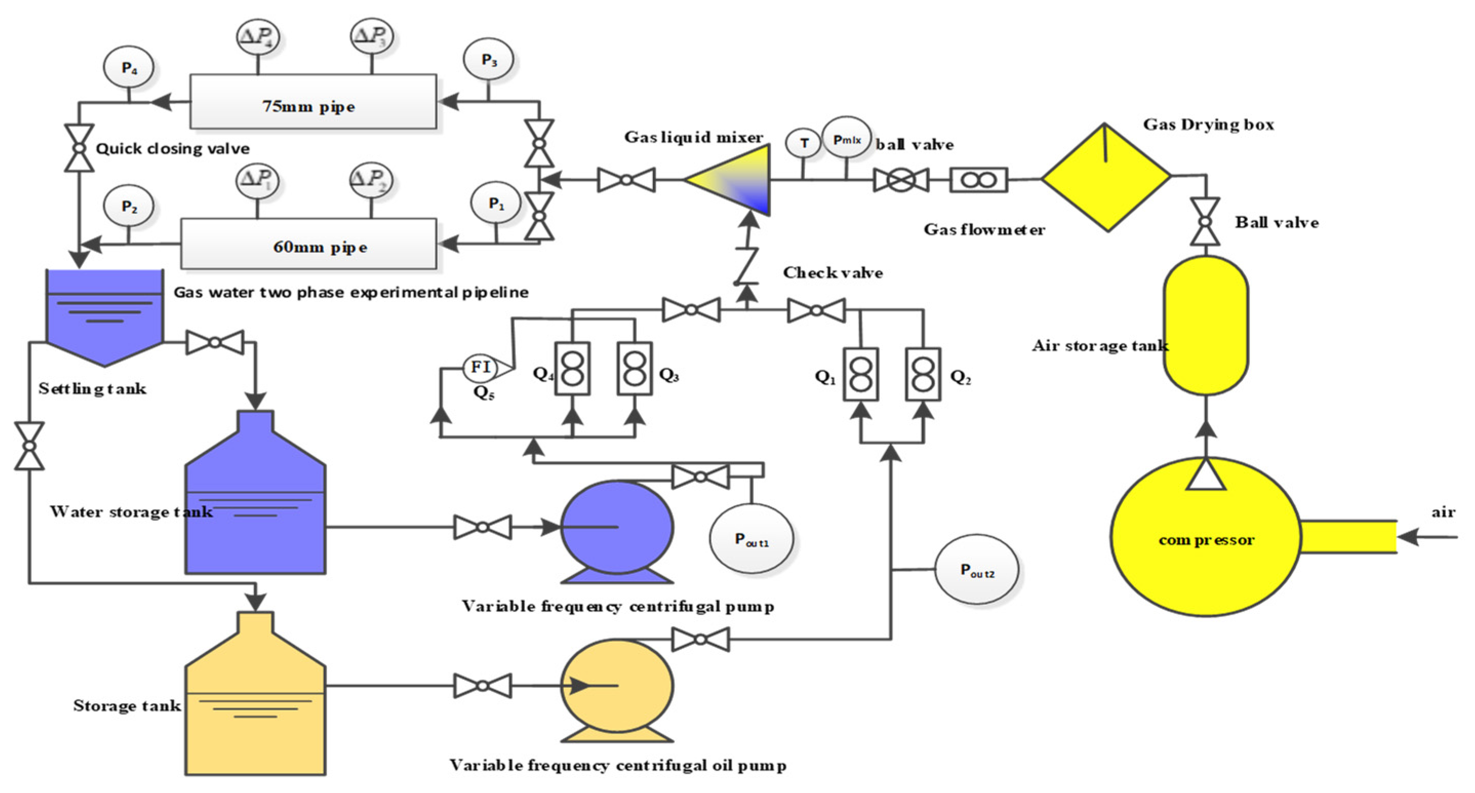
The experiment was carried out in the Key Laboratory of Multiphase Flow of PetroChina at Yangtze University. The experimental devices had 75 mm and 60 mm pipe diameters and a total length of 11.5 m. A pressure sensor, a temperature sensor, a differential pressure sensor, a quick closing valve, and other devices were installed on the pipe section. The distance between the two quick-closing valves was 9.5 m, including a 7 m plexiglass pipe and 2.4 m stainless-steel pipe [19]. The drain valve was used to place the liquid remaining in the wellbore after the quick-closing valve was closed into the measuring cylinder for a liquid-phase volume measurement to measure the liquid holdup, as shown in Figure 1.

The gas used in the experiment was air, and the liquid was tap water. The surface tension of water is about 72.8 mN/m at 20 °C, the densities of water and air are 1000 and 1.05 kg/m³, respectively, and the viscosities of water and air are 1 and 0.0181 mPa·s, respectively.

For different gas–liquid volumes and gas–liquid ratios, experiments on the variation law for the pressure drop under different conditions were carried out.

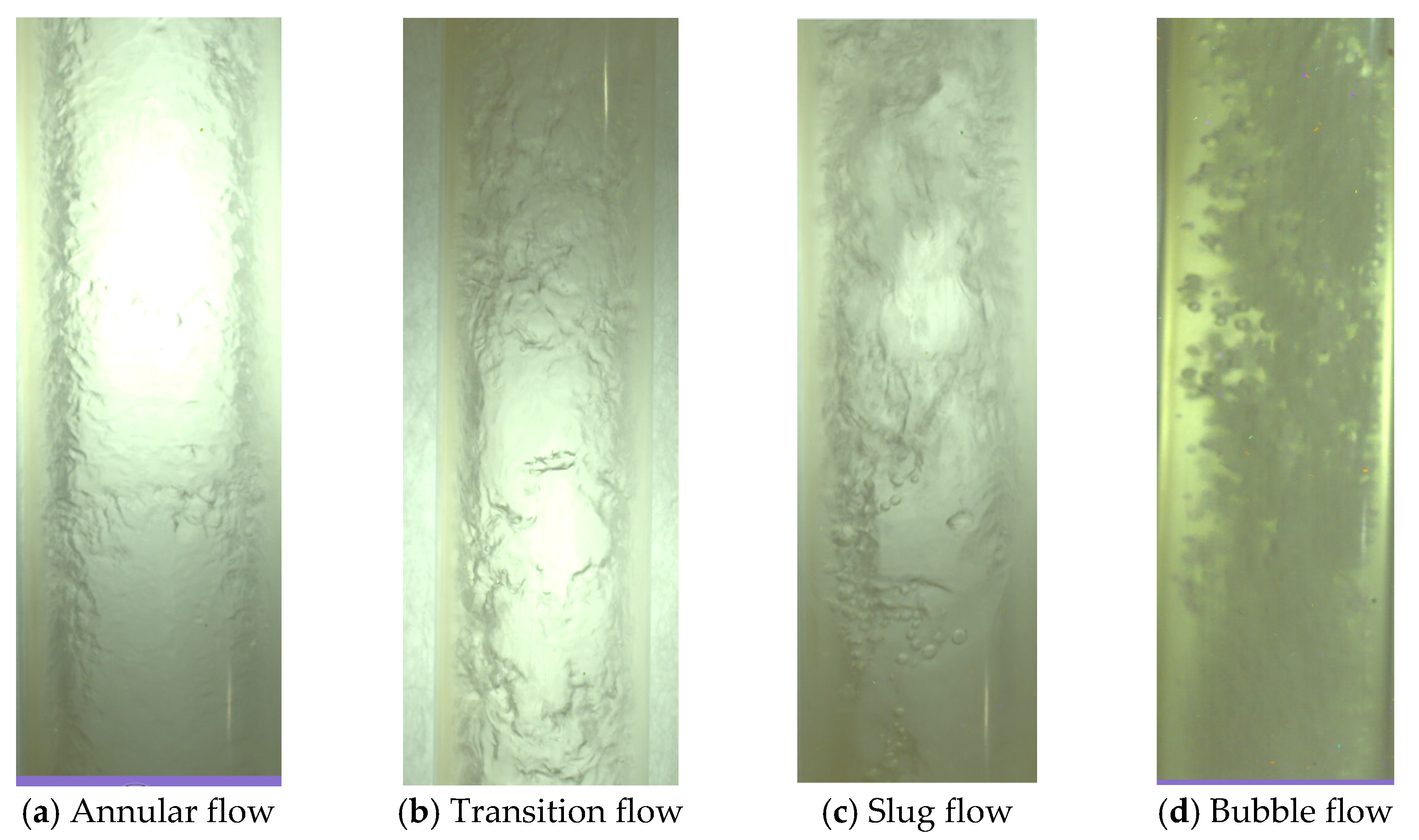
A total of 760 groups of gas–liquid flow pattern experiments with pipe section angles of 10°, 30°, 40°, 45°, 50°, 55°, 60°, 70°, and 90° were completed. By adjusting the gas–liquid ratio with a fixed amount of liquid, the physical experimental simulation of the flow pattern at different angles was carried out, and the bubble flow, slug flow, stirred flow, and annular flow were observed, respectively. The experimental gas-liquid range is shown in

Table 1. Experimental scope.

Experimental Content	Pipe Inclination	Gas Flow (m3/d);	Liquid Flow (m3/d);	Recorded Data	Group Number
Experiment for pressure drop law for 60 mm and 75 mm pipe diameters	10, 30, 40, 45, 50, 55, 60, 70, 90	Adjusted according to the flow pattern	10, 50, 100, 150, 200, 300	Flow pattern, pressure drop, liquid holdup	1003

.

The experimental picture is shown in Figure 2 below.

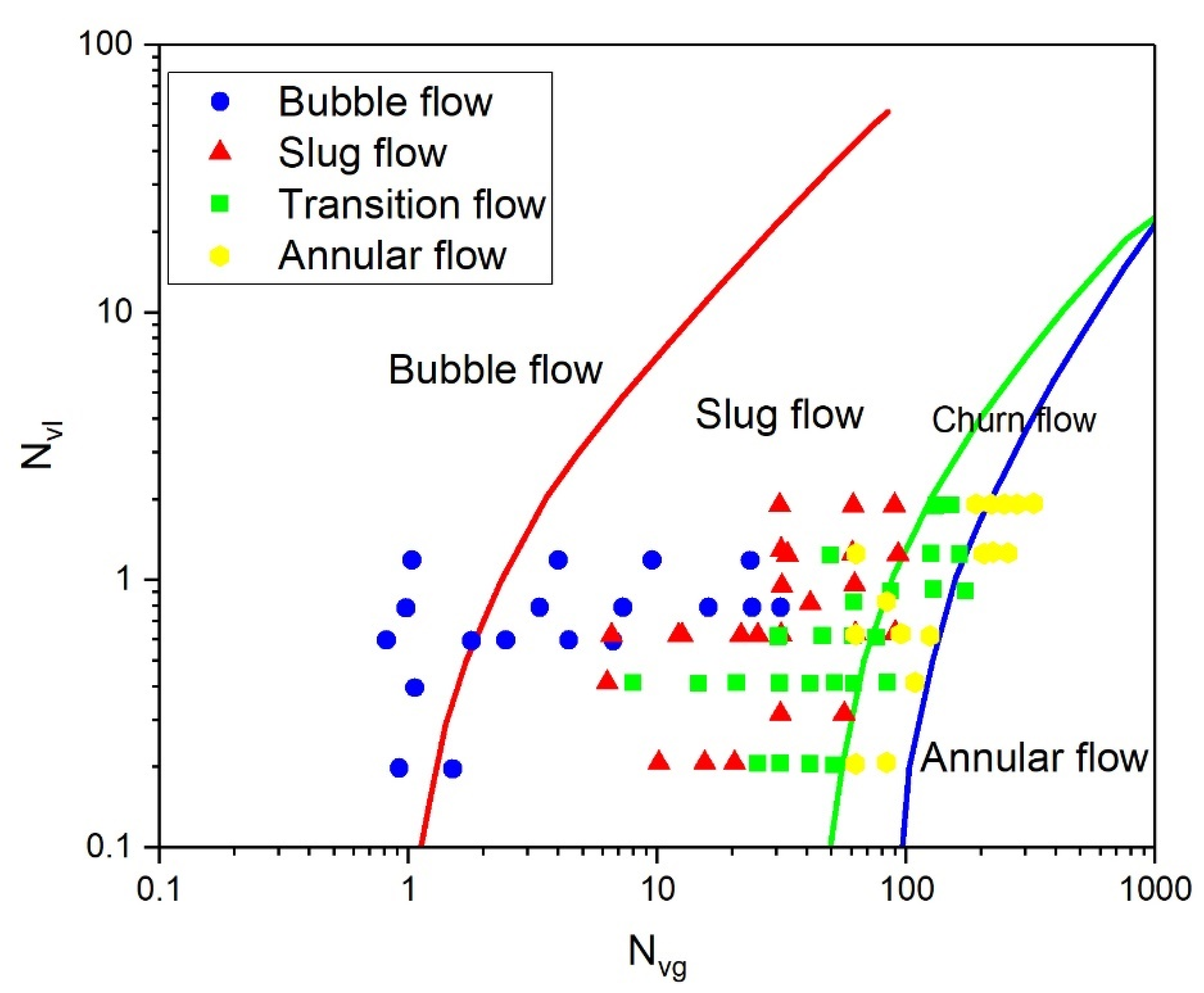
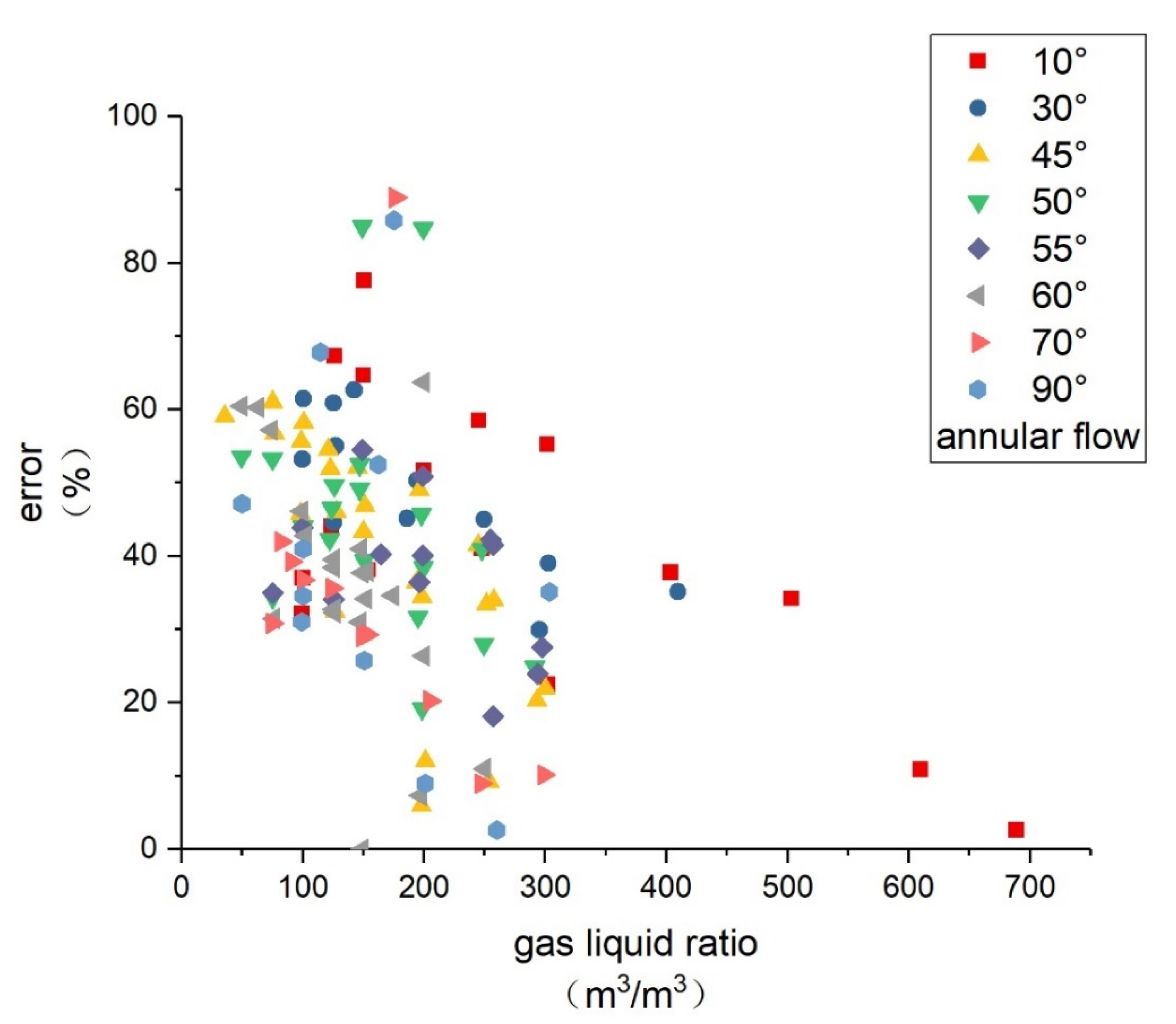
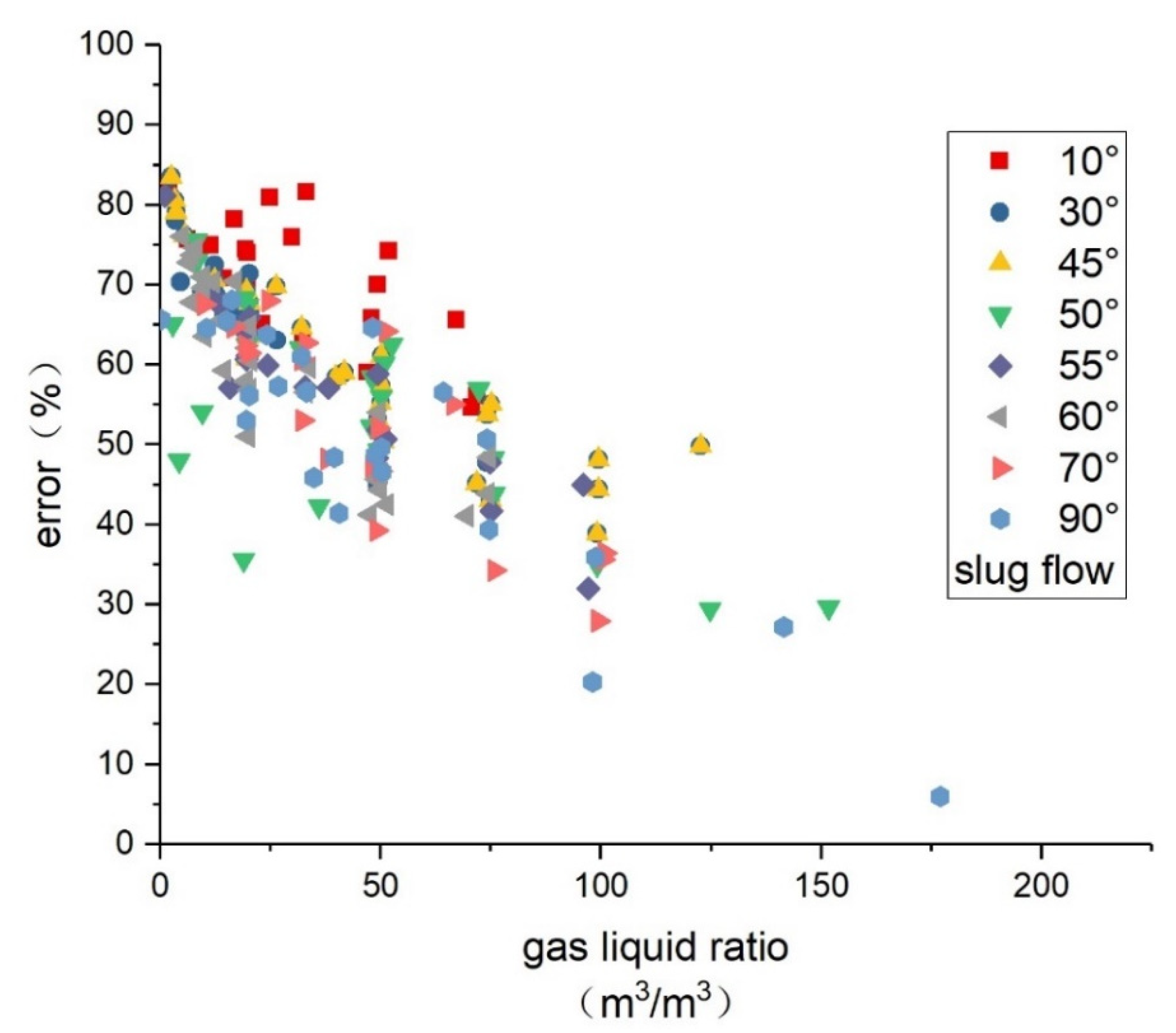
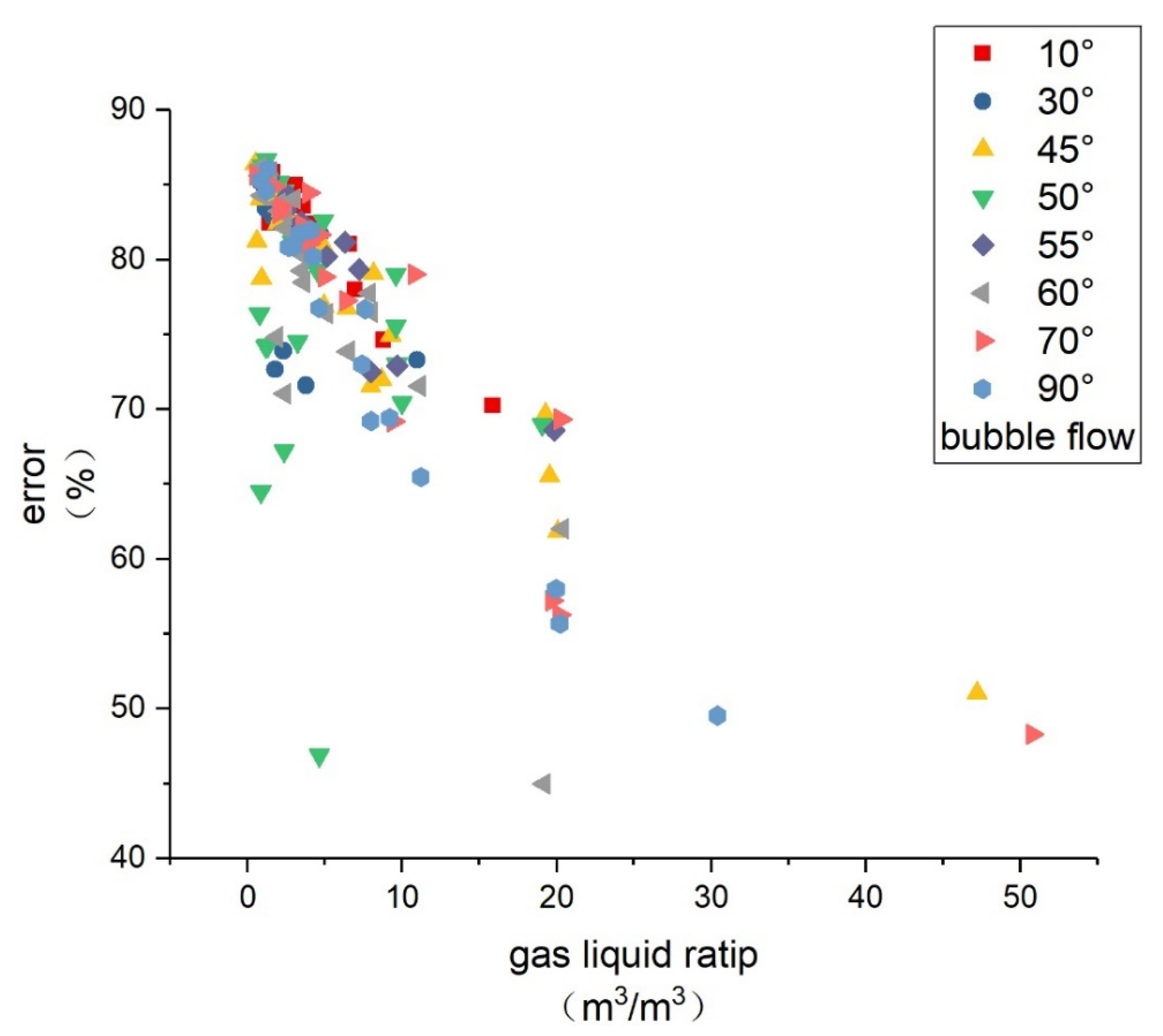
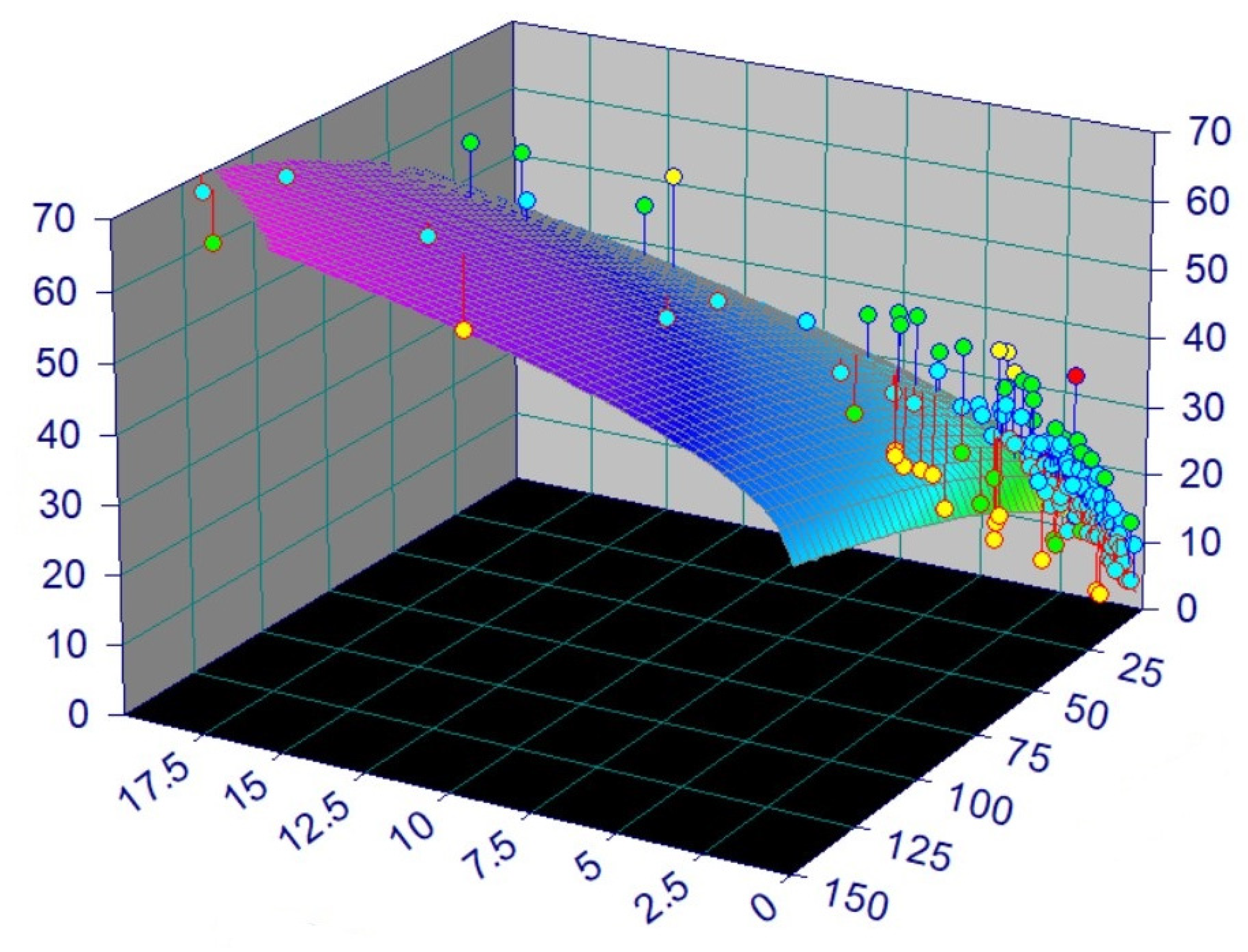
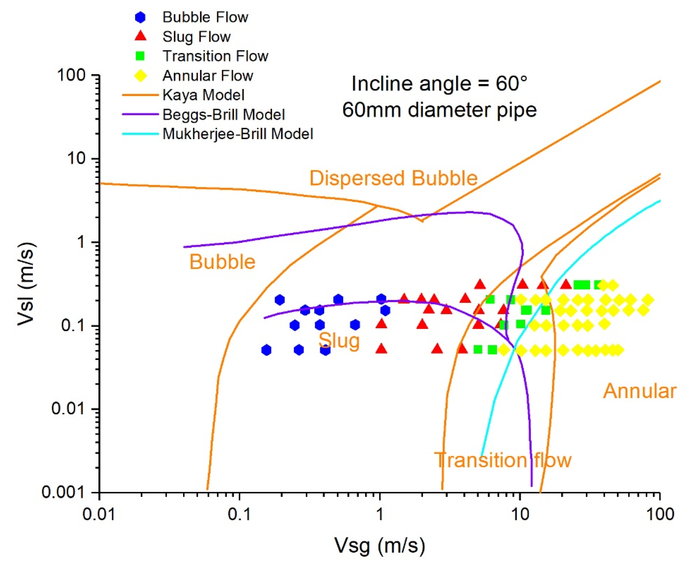
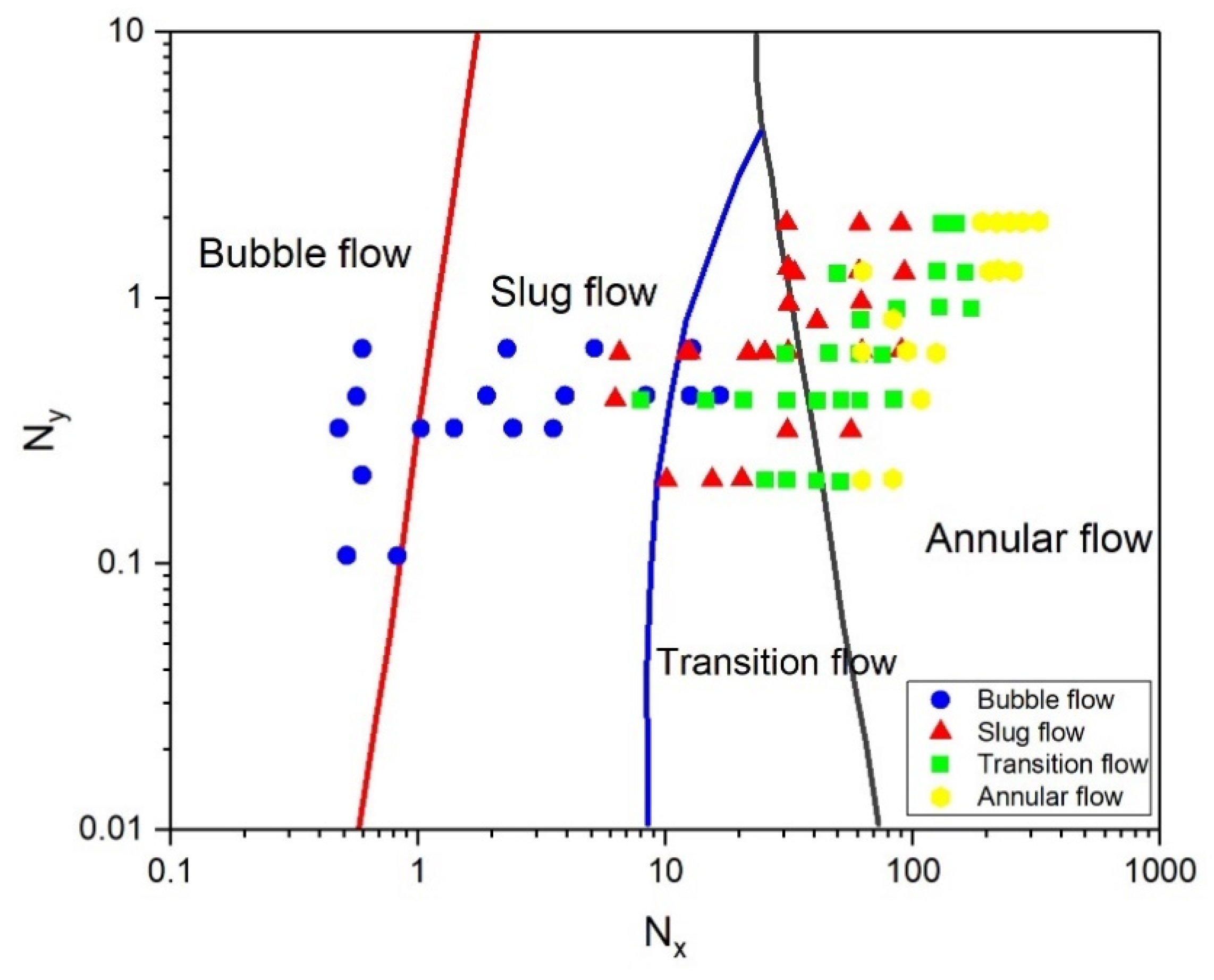
Through the observation of the experimental phenomenon of a large gas–liquid two-phase pipe flow, it was found that the change in flow pattern was slightly different from that for small flows. According to the experimental data for a large water volume and large air volume under experimental conditions, various commonly used flow pattern identification methods were screened. The preliminary screening result was that the Kaya–Sarica–Brill flow pattern identification method was more accurate in wellbore flow pattern identification for the Donghai gas field, as shown in Figure 3. The reason is that the change trend for the Kaya–Sarica–Brill model is basically consistent with the flow pattern boundary trend observed in the experiment.

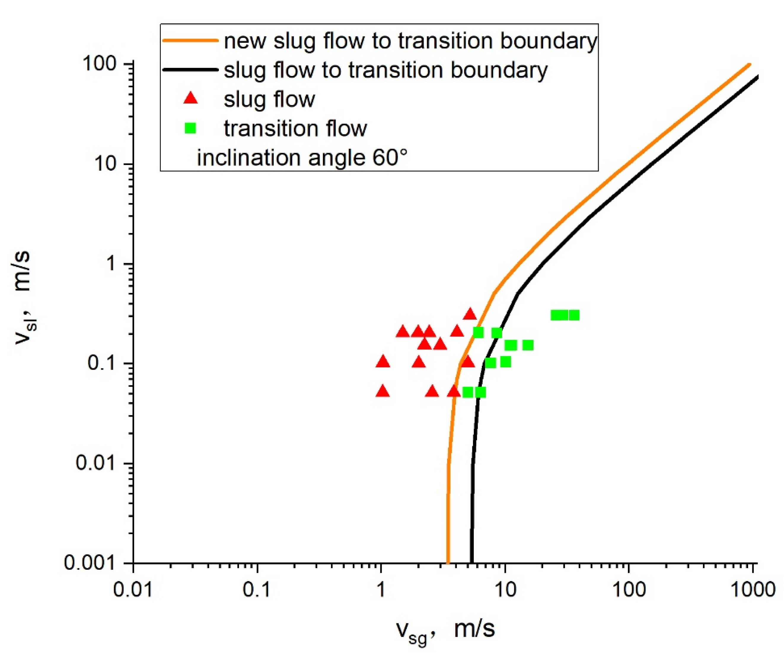
Considering that the basic data for using superficial gas velocity (vsg) and superficial liquid velocity (vsl) for flow pattern judgment are not comprehensive, the Aziz–Govier–Fogarasi model and Duns–Ros method [10] based on the speed criterion were also considered, as shown in Figure 4 and Figure 5. Since most of the applications of the Orkiszewski method use the Duns–Ros method for flow pattern discrimination, the Duns–Ros flow pattern discrimination method was verified using data.

Figure 4. Application of Aziz–Govier–Fogarasi model flow pattern discrimination formula.

Figure 4. Application of Aziz–Govier–Fogarasi model flow pattern discrimination formula.

Figure 5. Application of Duns–Ros flow pattern discrimination formula.

Figure 5. Application of Duns–Ros flow pattern discrimination formula.

$$N_x=3.28v_{sg}{\left(\frac{{\rho }_g}{{\rho }_a}\right)}^{1/8}{\left(\frac{{\rho }_l{\sigma }_w}{{\rho }_w\sigma }\right)}^{1/4}$$

$$N_y=3.28v_{sl}{\left(\frac{{\rho }_l{\sigma }_w}{{\rho }_w\sigma }\right)}^{1/4}$$

$$N_{vl}=v_{sl}\sqrt[4]{{\rho }_l/g\sigma }$$

$$N_{vg}=v_{sg}\sqrt[4]{{\rho }_l/g\sigma }$$

where

• $v_{sl}$ is the liquid superficial velocity, m/s;
• $v_{sg}$ is the gas superficial velocity, m/s;
• ${\rho }_l$ is the liquid density, kg/m³;
• ${\rho }_g$ is the gas density, kg/m³;
• $\sigma$ is the liquid-phase surface tension, mN/m;
• ${\rho }_a$ is the air density under standard conditions, kg/m³;
• ${\rho }_w$ is the water density under standard conditions, kg/m³;
• ${\sigma }_w$ is the water-phase surface tension, mN/m.

From Figure 3, Figure 4 and Figure 5, it can be observed that the change trend for the Kaya–Sarica–Brill model is roughly the same as that for the experimental data. Finally, the Kaya–Sarica–Brill model was still selected as the basis for the flow pattern discrimination formula for correction.

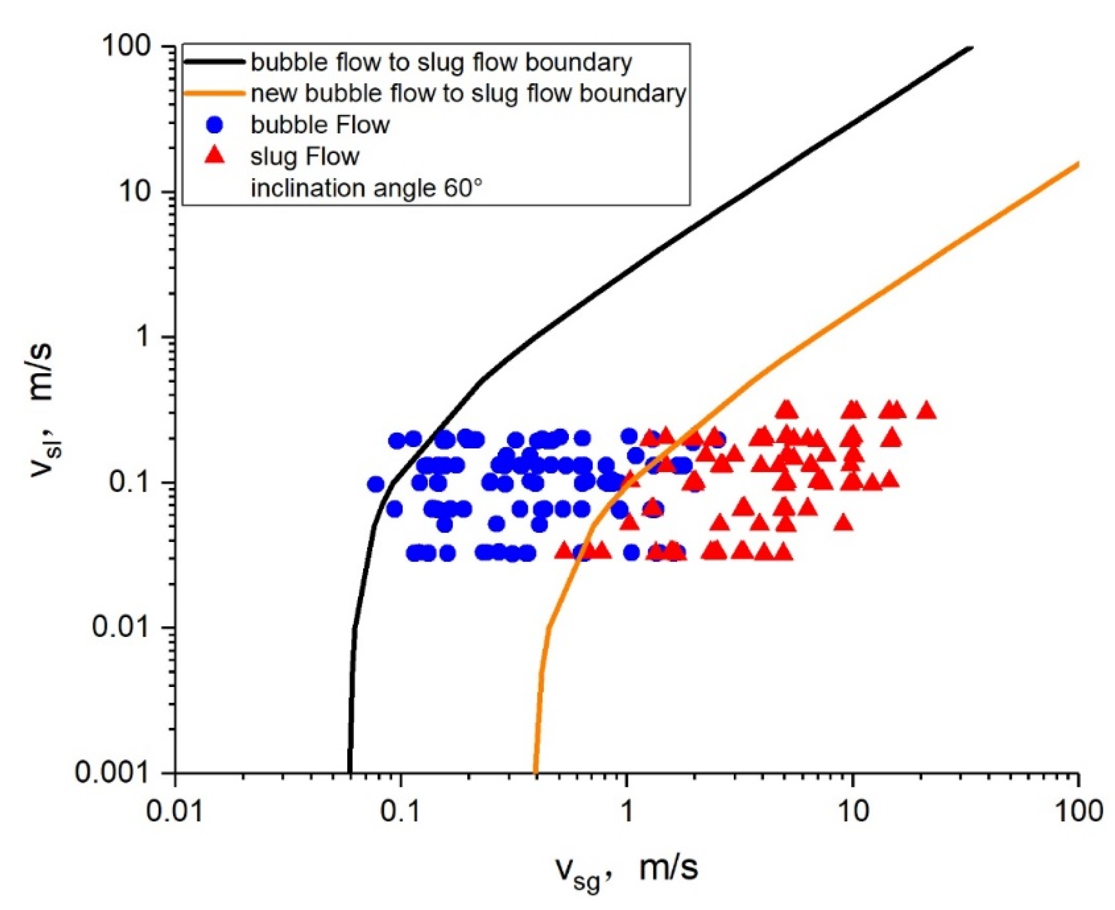
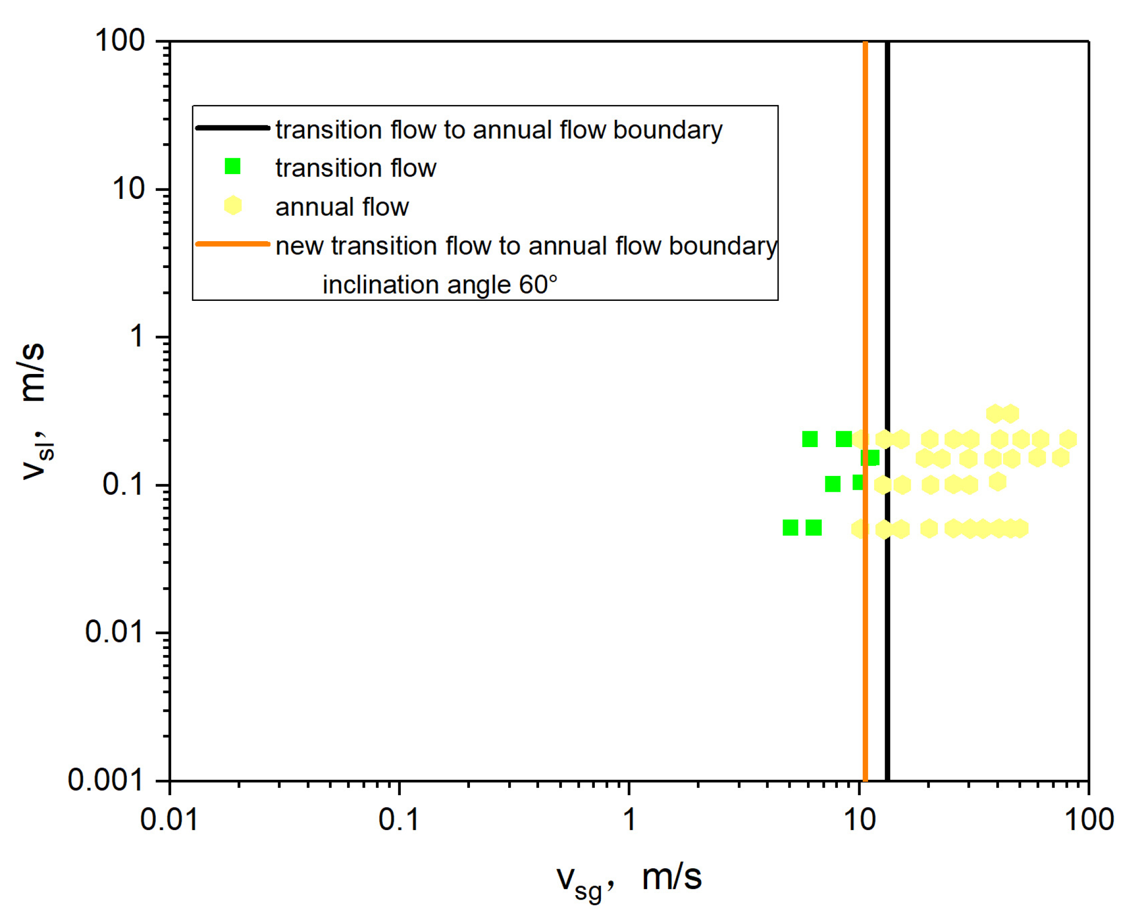
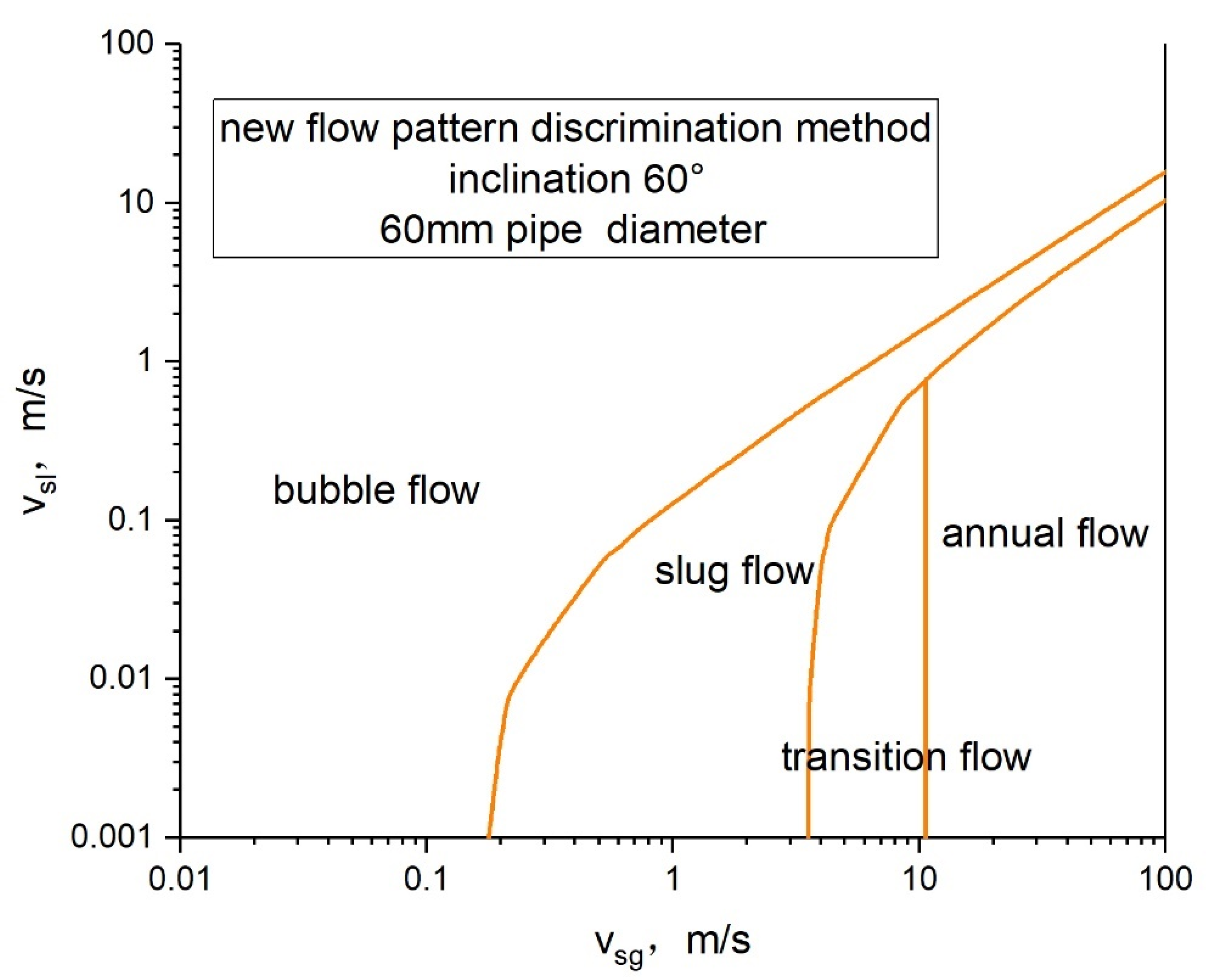
The experimental data were introduced to the Kaya–Sarica–Brill model and shown below. The flow pattern was small under the condition of large flow, and the prediction was often inaccurate.

After fitting, the new boundaries of each flow-pattern discrimination were as shown in Figure 6, Figure 7, Figure 8 and Figure 9 (taking 60° as an example):

The new flow pattern discrimination formula is as follows:

The boundary of the bubble slug flow pattern transition:

$$v_{sg}=6.4v_{sl}+2.5{\left[\frac{g\sigma \left({\rho }_l-{\rho }_g\right)}{{\rho }_l^2}\right]}^{0.25}\sqrt{sin\theta }$$

(1)

The boundary of the flow pattern transition between slug flow and stirred flow:

$$v_{sg}=7.8\left[1.2v_{sl}+\left(0.35sin\theta +0.54cos\theta {\left(\frac{g\left({\rho }_l-{\rho }_g\right)D}{{\rho }_l}\right)}^{0.5}\right)\right]$$

(2)

The boundary of the flow pattern transition between stirred flow and annular flow:

$$v_{sg}=3.1{\left[\frac{\sigma g\left({\rho }_l-{\rho }_g\right)}{{\rho }_g^2}\right]}^{0.25}$$

(3)

where

• $v_{sl}$ is the liquid superficial velocity, m/s;
• $v_{sg}$ is the gas superficial velocity, m/s;
• $\sigma$ is the liquid-phase surface tension, mN/m;
• $\theta$ is the pipe and horizontal inclination angle, °.

The new flow-pattern-discrimination formula is as follows:

3. Calculation Formula for Liquid Holdup

Through the analysis of 760 groups of gas–liquid flow pattern experiments under different angles, the accuracy of the liquid holdup calculation formula under different flow patterns and flow patterns was verified, respectively.

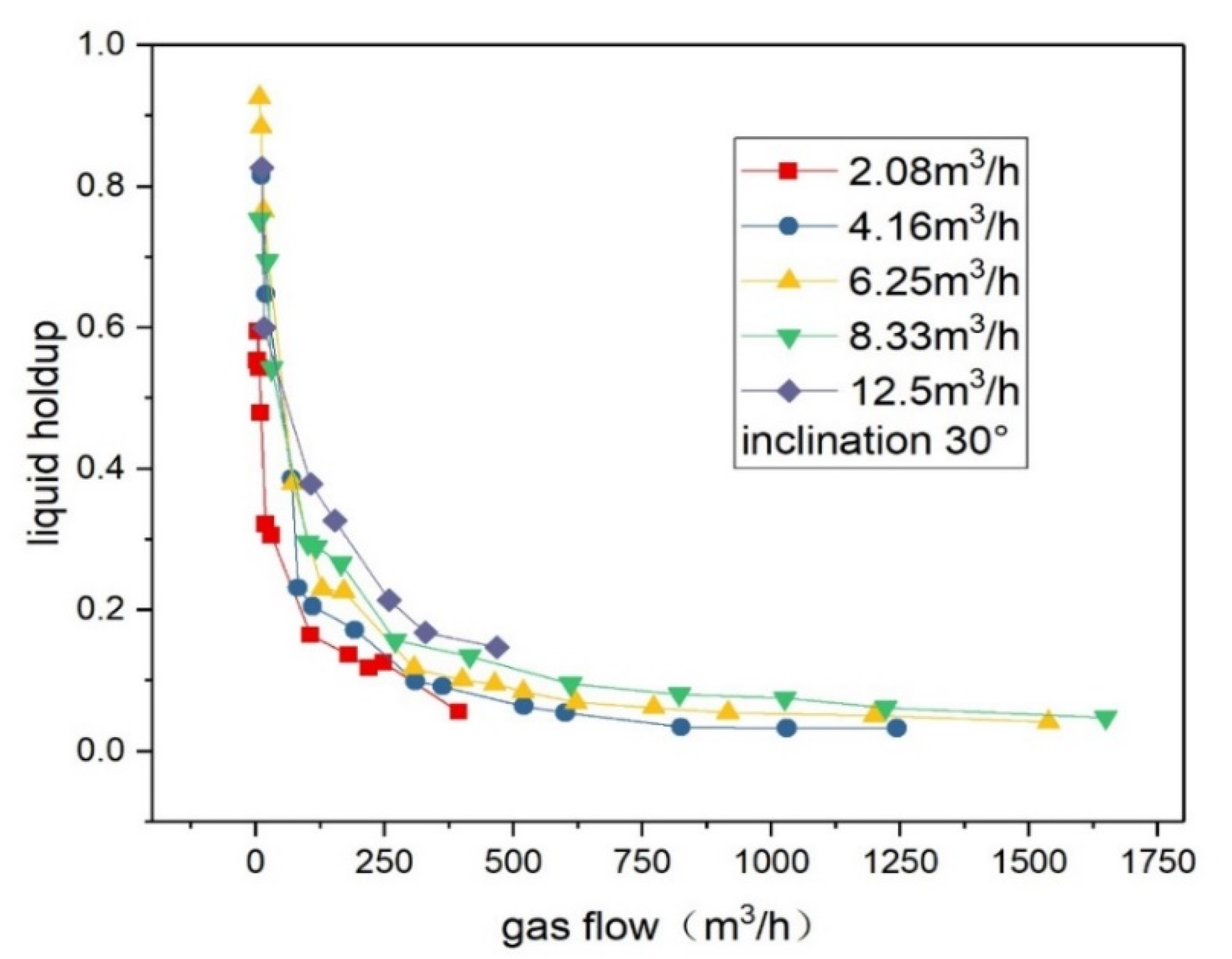
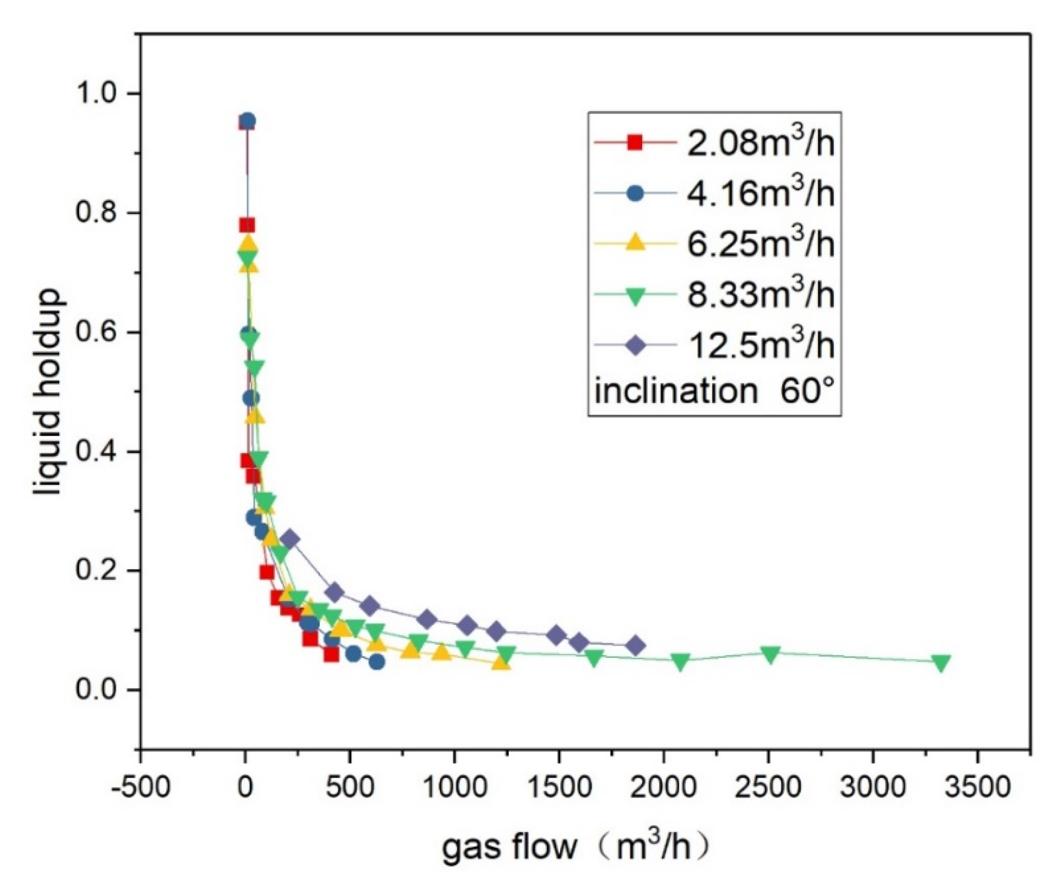
By sorting and analyzing the experimental data, the law of change for the liquid holdup under different conditions was drawn, shown in Figure 10 and Figure 11. It can be seen from the figure that, under the same liquid flow condition, the liquid holdup rate decreases with an increase in the gas flow rate. Under the same gas flow rate condition, the liquid holdup rate gradually increases with an increase in the liquid flow rate, but the change is not significant.

There are many methods for calculating the liquid holdup. The Mukherjee and Brill method was established to calculate the liquid holdup, and the Beggs and Brill model also puts forward a calculation method for the liquid holdup. However, when the B–B method is used to calculate the liquid holdup of different flow patterns, there is discontinuity, so it is difficult to ensure the accuracy of the liquid holdup calculation [19,20,21]. The empirical formula provided by the Mukherjee and Brill method has good continuity, considers the influencing factors comprehensively, and is suitable for all flow patterns at all angles.

$$H_l=exp\left[\left(c_1+c_{2}sin\theta +c_{3}si{n}^2\theta +c_4{N}_l^2\right)\frac{N_{vg}^{c_5}}{N_{vl}^{c_6}}\right]$$

(4)

$$N_{vl}=v_{sl}{(\frac{{\rho }_l}{g\sigma })}^{0.25}$$

(5)

$$N_{vg}=v_{sg}{(\frac{{\rho }_l}{g\sigma })}^{0.25}$$

(6)

$$N_l={\mu }_l{(\frac{g}{{\rho }_l{\sigma }^3})}^{0.25}$$

(7)

where

• $v_{sl}$ is the apparent velocity of the liquid phase, m/s;
• $v_{sg}$ is the apparent velocity of the gas phase, m/s;
• $\sigma$ is the surface tension of the liquid phase, N/m;
• ${\mu }_l$ is the viscosity of the liquid phase, Pa·s.

Based on the good continuity of the Mukherjee correlation equation for the liquid holdup and comprehensive consideration of factors, the empirical constant in the relationship was chosen to be revised. 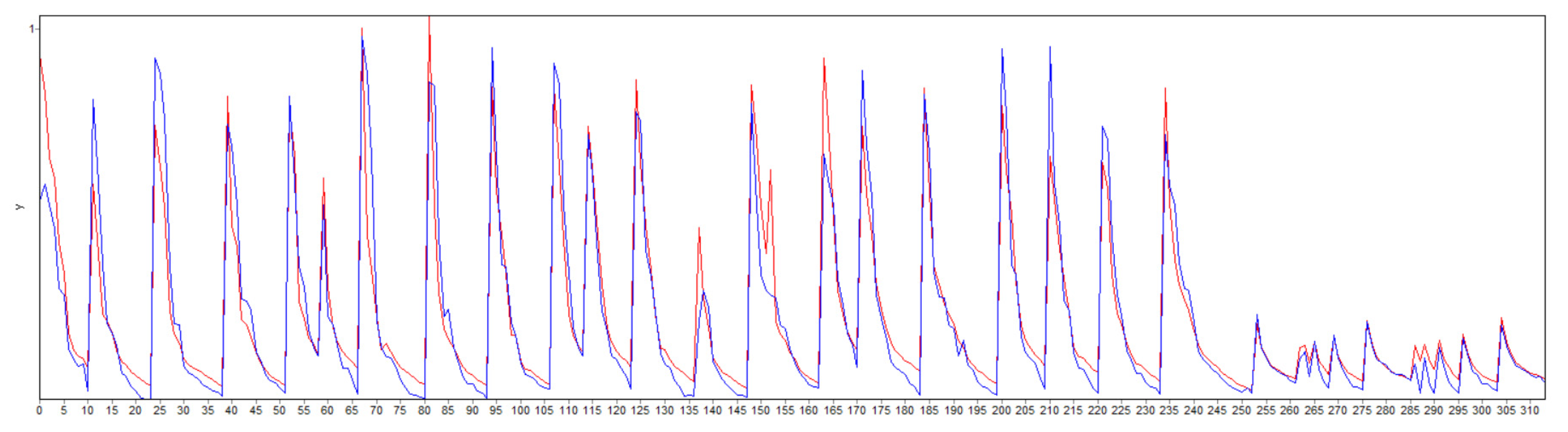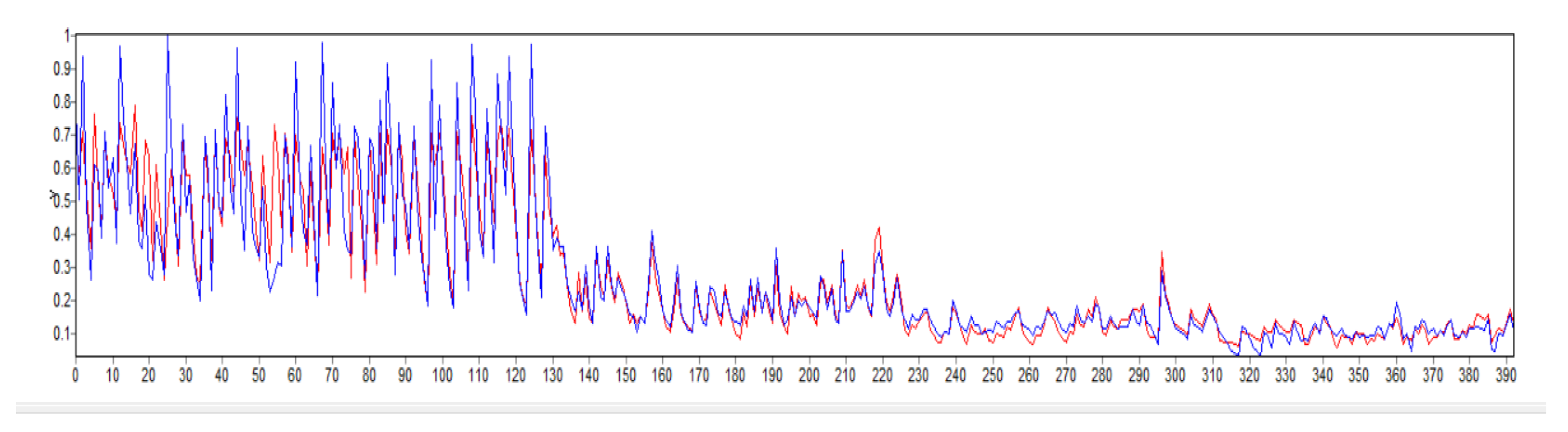According to the liquid holdup formula for gas–liquid two-phase flows provided by Mukherjee and Brill, the relationship between the experimental liquid holdup H_l and the correlation criteria N_vl, N_vg, and N_l provided by Mukherjee and Brill was fitted. A comparison between the corrected calculated values and the actual values is shown in Figure 12 and Figure 13.

The blue line represents the fitted value, and the red line represents the experimental value. The x-axis represents the number of iterations, and the y-axis represents the value of the result.

The new empirical constant obtained by fitting and the corrected liquid holdup error are shown in

Table 2. Parameters of the newly established liquid holdup calculation model.

Pipe Diameter (mm)	${\mathit{c}}_1$	${\mathit{c}}_2$	${\mathit{c}}_3$	${\mathit{c}}_4$	${\mathit{c}}_5$	${\mathit{c}}_6$
75	−0.2373	−0.1255	0.1042	−0.38899	0.3911	0.02645
60	−0.2351	0.075873	−0.0644	−0.35134	0.447652	0.084494

and

Table 3. Comparison of calculation error for the liquid holdup of the new model with that of the M–B model.

Dip Angle	Mukherjee and Brill 60 mm	New 60 mm	New 70 mm
30	0.4946	0.07267	−0.08156
45	0.55558	0.15683	−0.10785
50	0.44901	−0.0296	0.015428
55	0.56247	−0.11359	−0.05958
70	0.78502	−0.156	−0.0094
90	0.79817	−0.09629	0.086091

, respectively.

4. Pressure Calculation Formula

Based on the accurate establishment of the liquid holdup calculation model and flow pattern discrimination method, the pressure drop calculation formula was optimized and established.

In the Beggs and Brill pressure drop calculation model, the calculation of the friction coefficient is related to the flow pattern [3]. Therefore, this coefficient is used as the main correction parameter. During this test, the flow ranges of the gas and liquid phases were relatively large, and the experimental phenomena covered all the flow pattern areas; corresponding calculation methods for drag coefficients along the way were provided for different flow patterns.

$$\frac{dp}{dz}=\frac{\left[{\rho }_l{H}_l+{\rho }_g\left(1-H_l\right)\right]gsin\theta +\frac{\lambda Gv}{2DA}}{1-\left\{\left[{\rho }_l{H}_l+{\rho }_g\left(1-H_l\right)\right]v{v}_{sg}\right\}/p}$$

(8)

The drag coefficient of the gas–liquid two-phase flow was obtained according to the Beggs and Brill model.

$$\lambda ={\lambda }^{\prime }{e}^s$$

(9)

In the formula

$${\lambda }^{\prime }={\left[2lg\left(\frac{R{e}^{\prime }}{4.5223lgR{e}^{\prime }-3.8215}\right)\right]}^{-2}$$

(10)

$$R{e}^{\prime }=\frac{Dv\left[{\rho }_l{E}_l+{\rho }_g\left(1-E_l\right)\right]}{{\mu }_l{E}_l+{\mu }_g\left(1-E_l\right)}$$

(11)

• ${\lambda }^{\prime }$ is the “no slip” drag coefficient along the way, dimensionless;
• s is the index;
• $R{e}^{\prime }$ is the Reynolds number without slip;
• ${\mu }_l$ and ${\mu }_g$ are the viscosities of the liquid phase and gas phase, Pa·s.

The index s in the formula can be calculated according to the following formula:

$$s=\frac{lnY}{-0.0523+3.182lnY-0.8725{\left(lnY\right)}^2+0.01853{\left(lnY\right)}^4}$$

(12)

$$Y=\frac{E_l}{{\left[H_l\left(\theta \right)\right]}^2}$$

(13)

After verifying the B–B model with the data under the condition of the gas–liquid ratio in the laboratory, it was found that the error was large, and the average absolute deviation is shown in

Table 4. The calculation error for the B–B model applied to the atmospheric liquid flow.

Error	10°	30	45	50	55	60	70	90
Bubble flow	81.34%	78.13%	77.92%	77.24%	77.17%	77.39%	75.72%	73.86%
Slug flow	69.43%	62.3%	59.92%	55.11%	54.52%	54.04%	51.98%	49.7%
Transition flow	56.07%	57.00%	49.83%	48.63%	45.64%	47.41%	38.24%	27.97%
Annular flow	50.73%	48.54%	40.06%	45.42%	37.57%	36.49%	33.72%	33.64%

.

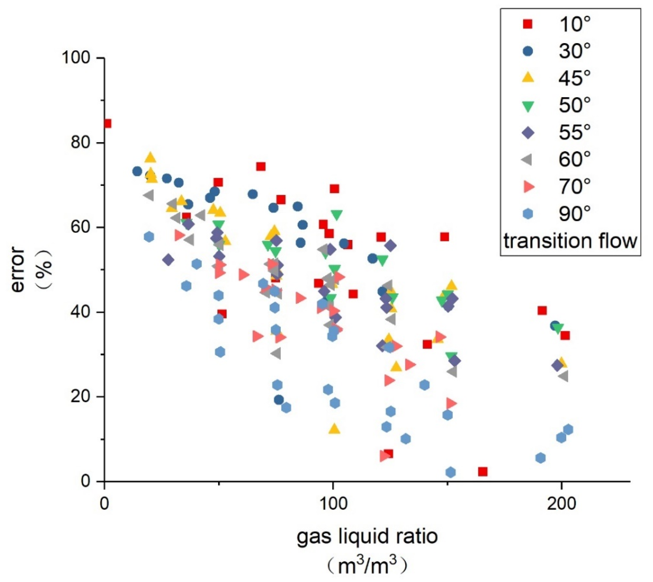
As shown in Figure 14, Figure 15, Figure 16 and Figure 17, it can be observed from the error analysis diagram that, although the distribution of the data points is irregular, the overall trend is that the error of the B–B model decreases with an increase in the gas–liquid ratio. This phenomenon is also mentioned in Chen Dechun’s research [18]. The error of the B–B model is better when the gas–liquid ratio is low. However, he mainly used the field data to evaluate the existing model and did not propose a solution. Moreover, the analysis of the existing model used the field-measured data, there was a lack of wellbore flow data for large water volume gas wells, and the evaluation focused on the data with a gas–liquid ratio of more than 1750. With an increase in the gas–liquid ratio, the error of the B–B model will decrease significantly. Since the error decreases with an increase in the gas–liquid ratio, the dimensionless number that can characterize the gas–liquid flow is considered to re-establish the formula.

The Froude number (FR) is a dimensionless scalar in fluid mechanics; it is the ratio of the fluid kinetic energy to potential energy. When fr > 1, the water depth is small, and the velocity is turbulent. Similarly, when fr < 1, the velocity is slow, and the water depth is large. Similarly, the Reynolds number (Re) is also a classical dimensionless number used to characterize fluid flows in fluid mechanics. The gas–liquid velocity ratio is a more intuitive reaction gas–liquid ratio. In addition to the gas–liquid velocity ratio, the Froude number and Reynolds number can also characterize the effect of fluid flows from the side [22,23,24,25,26]. In order to improve the calculation accuracy for the pressure drop calculation formula, the three parameters of the Froude number, Reynolds number, and gas–liquid velocity ratio were brought into the model for correlation verification, and the most appropriate parameters representing the gas–liquid ratio were selected for the establishment of a new model.

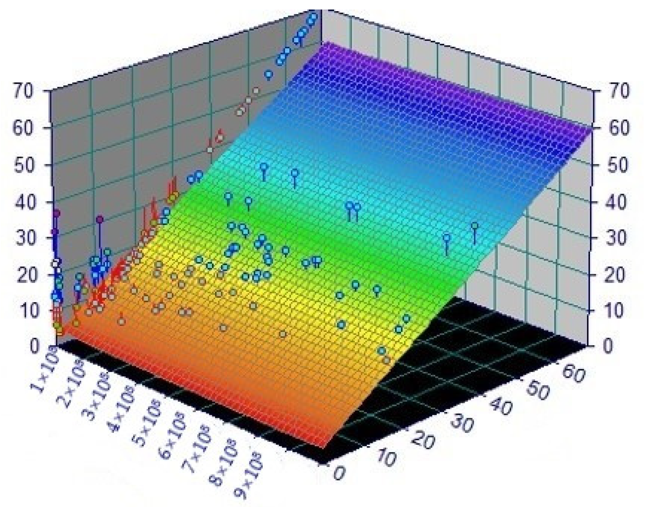
According to the pressure drop data for gas–liquid two-phase pipe flows with large amounts of water and gas obtained under the experimental conditions, the gas–liquid ratio was introduced, combined with the pressure drop calculation formula of the B–B model, and the correlation was verified according to the experimental data. The correlation coefficient obtained using the new formula was r = 0.81. The correlation between the calculated value and the actual value for the new formula is shown in Figure 18.

By introducing the Froude number and combining it with the pressure drop-calculation formula of the B–B model, the correlation between the Froude number and the calculation results for the B–B model was verified according to the experimental data. The correlation coefficient of the Froude number was r = 0.83, and the correlation between the calculated value and the actual value for the new formula is shown in Figure 19.

By correlating the Reynolds number with experimental data and the B–B model, it was found that the Reynolds number had a better correlation after fitting than the gas–liquid ratio and Froude number, as shown in Figure 20. Therefore, the Reynolds number was selected as the dimensionless number for characterizing the gas–liquid ratio for the optimization of the new model:

The above figure shows the correlation verification based on the optimal relationship automatically fitted by the TableCurve software. The correlation verification can be used for the three parameters of the Froude number, gas–liquid ratio, and Reynolds number as the parameters for characterizing the gas–liquid ratio, which can be applied to the adaptability screening in the optimization of the B–B model (selecting the optimal parameters through the order of correlation R under the recommended optimal relationship). Finally, the Reynolds number was selected and brought into the B–B model, and it was refitted according to the relationship obtained using TableCurve. For different angles and different flow patterns, the relationship is as follows:

$$\beta =d+e\times sin\theta +f\times si{n}^2\theta$$

(14)

$$∆p=a-bln{R}_e+\left\{\left[{\rho }_l{H}_l+{\rho }_g\left(1-H_l\right)\right]gsin\theta +c\times \beta \frac{\lambda Gv}{2DA}\right\}$$

(15)

The above formula was fitted with experimental data, and the pressure drop formula under each flow pattern was fitted with the Levenberg Marquardt method + general global optimization method. The new parameters are shown in

Table 5. Coefficient regression in the new model.

Flow pattern	a	b	c	d	e	f
Bubble flow	−10,603.7	909.117	0.14534	1.215	21.26	−28.4715
Slug flow	−4718.9	406.453	0.596	0.58	−2.014	1.9846
Transition flow	−6152.655	518.66	0.0334	2.6618	−10.015	9.729
Annular flow	−9429.522	740.94	0.01825	0.38156	1.376	−0.901

.

5. Field Data Verification

In the evaluation and optimization of the pressure drop calculation model for gas–liquid two-phase pipe flows in gas wells, Chen Dechun used the pressure measurement data for 102 wells in China and other countries. He conclude that “the gray model is applied to domestic gas wells and the calculated value is too small, while the gray model is applied to foreign gas wells, the calculation result is more accurate”. Since Chen Dechun has discussed the Gray model, the Gray model will not be discussed in this article. Comparing the gas well data selected by Chen Dechun, there is no significant change in gas production, and the gas–liquid ratio ranges from 444.4~75,000 m³/m³ to 2119.5~200,796.0 m³/m³. This shows that some pressure drop calculation models will not be applicable at high liquid volumes.

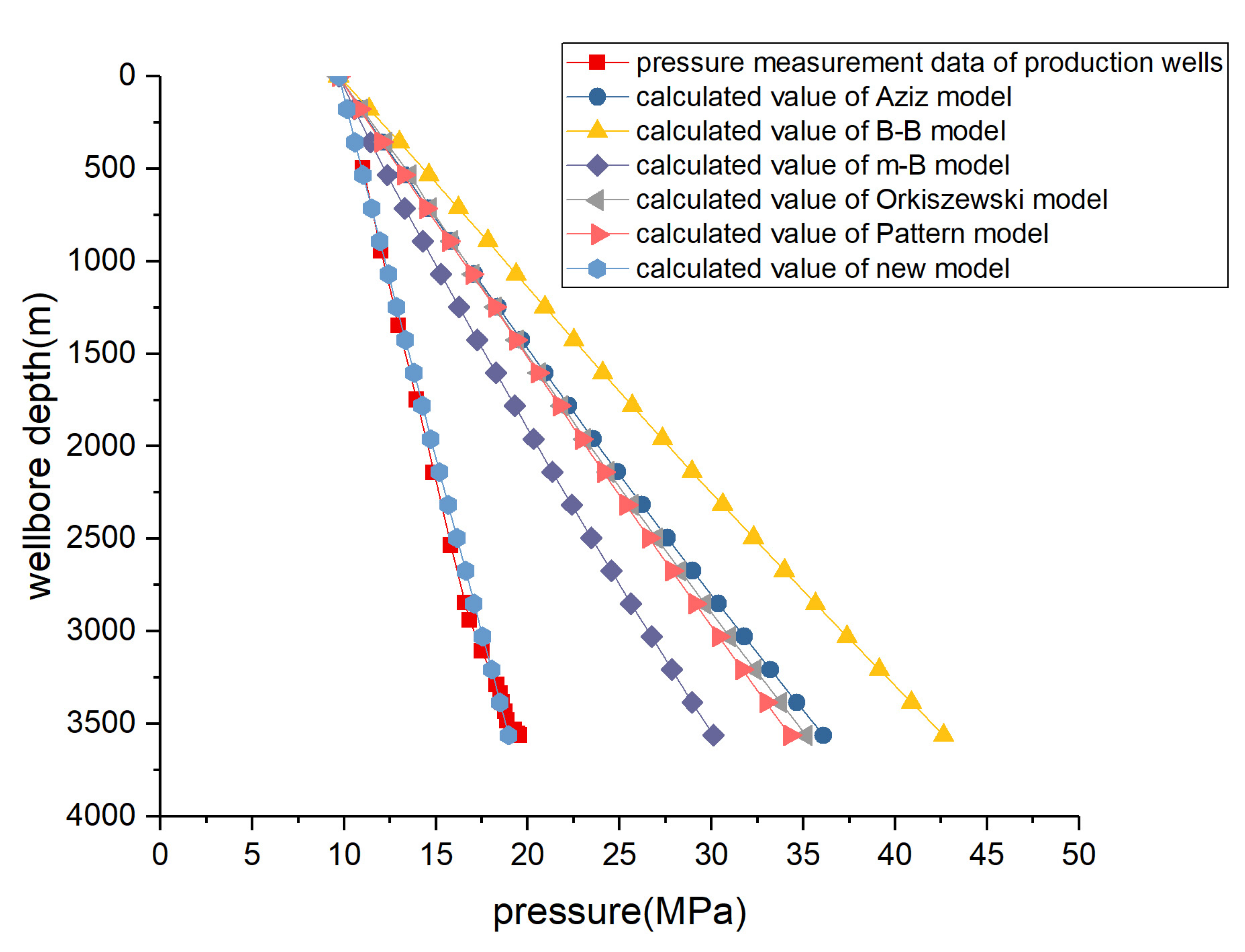
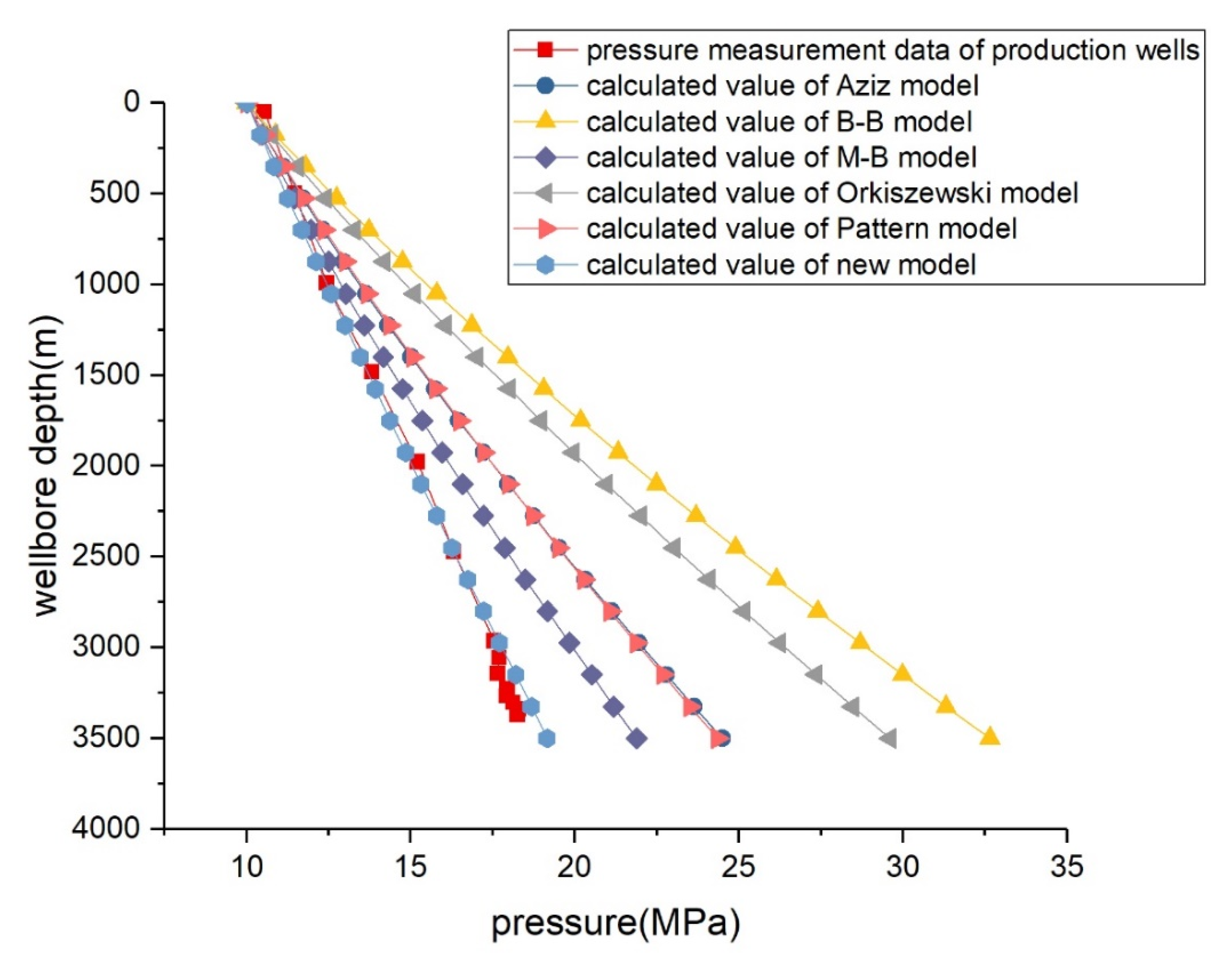
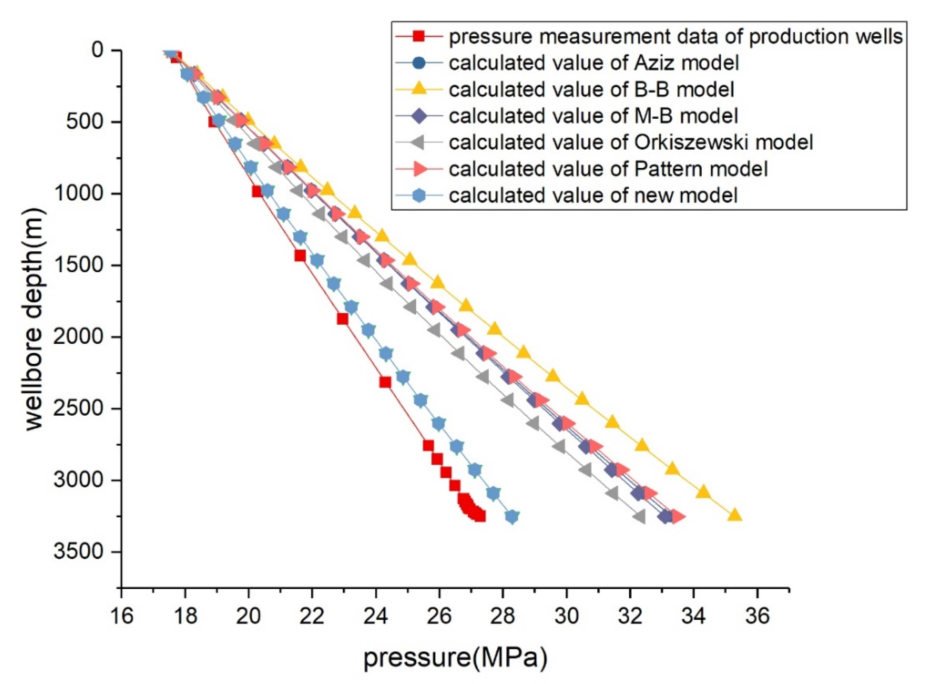
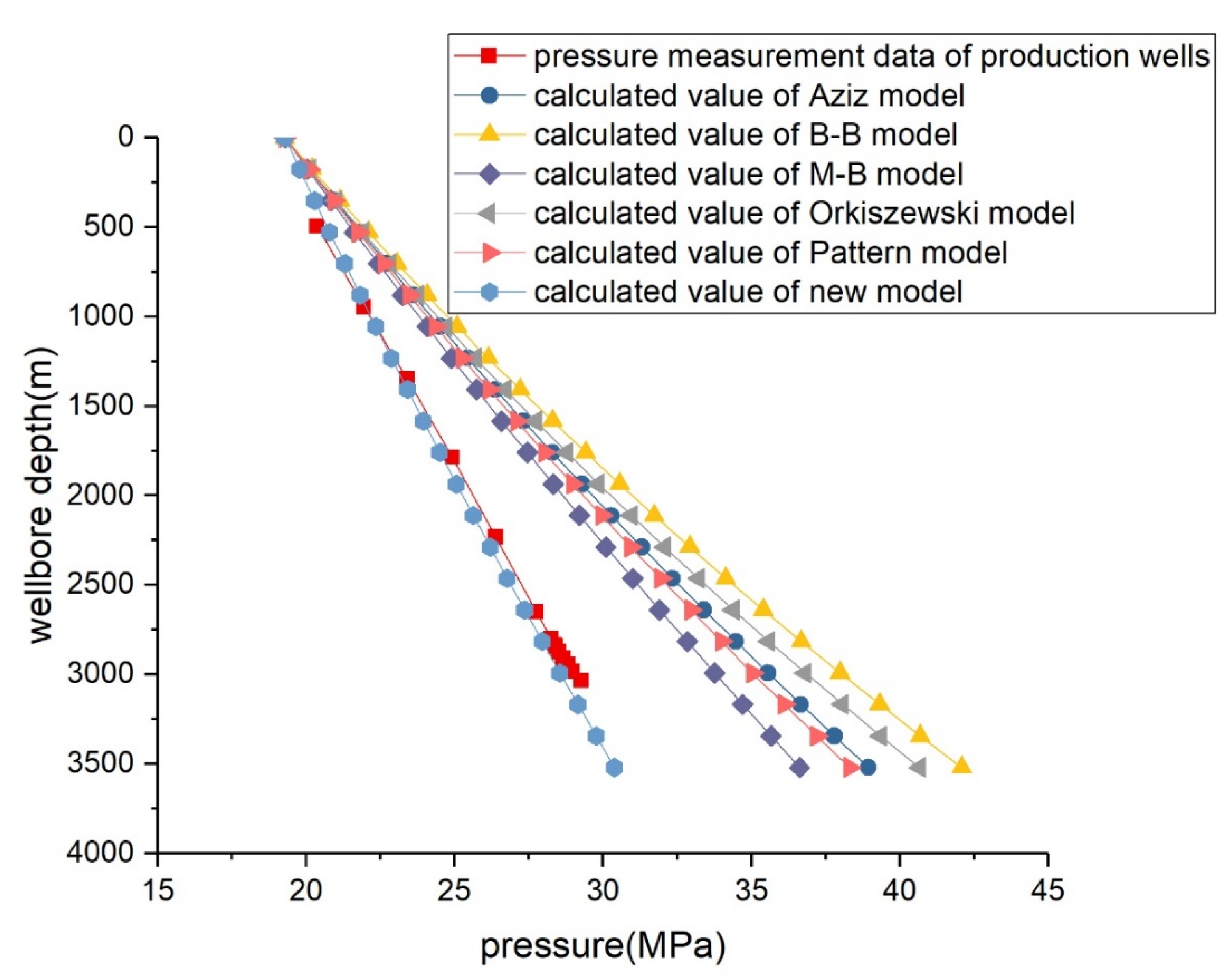
The results of the comparison between the calculated and measured values of the wellbore pressure distributions of six models are shown in Figure 21, Figure 22, Figure 23 and Figure 24. It can be observed from that the calculated values of the Aziz–Govier–Fogarasi model, Orkiszewski model, Hasan model, B–B model, pattern model, and M–B model are too large, and the predicted results of the new model are close to the actual values. The reason the error of these models is too large is that the water production of the Donghai gas field is huge, and the daily liquid production of a single well can reach 300 square meters. As the influence of the gas–liquid ratio on the pressure drop was not considered, the calculation of the above pressure drop model will be inaccurate.

The errors between different models are shown in

Table 6. Comparison of calculation errors of different models.

Absolute Error	Well 1	Well 2	Well 3	Well 4
Aziz–Govier–Fogarasi	62.26%	14.49%	29.92%	14.27%
B–B model	87.81%	19.24%	34.35%	38.36%
Hasan model	58.08%	5.45%	18.30%	7.85%
M–B model	40.03%	10.93%	29.66%	7.21%
Orkiszewski model	59.72%	16.76%	27.02%	29.99%
Pattern model	57.47%	13.42%	30.27%	14.232%
New model	1.6%	1.24%	18.3%	1.71%

.

6. Conclusions

Indoor experiments were used to simulate the production status of gas wells under the conditions of large water content and large gas production. It was verified from the aspects of the flow pattern, liquid holdup, and pressure drop that the current model has the problem of inaccurate prediction when applied to large-volume production gas wells. The flow pattern, flow pattern discrimination method, liquid holdup calculation method, and pressure drop calculation method for a large flow range were optimized using indoor experimental data. After analyzing the calculation error of the B–B pressure calculation model when applied to atmospheric liquid flow, it was found that the error of the B–B model increased with an increase in the gas–liquid ratio and increased with a decrease in the angle. In terms of innovation, through many experimental data, the distribution law for the convection type and the calculation method for liquid holdup were optimized, and it was found that the B–B model is not applicable under the production condition of a large water well. Based on the experimental data, the distribution law for the pressure drop calculation error was analyzed. The calculated value, actual value, and possible influencing factors were analyzed using the TableCurve software. It is concluded that the introduction of the Reynolds number can greatly improve the calculation accuracy. On the basis of considering the influence of the angle and gas–liquid ratio on the calculation accuracy for the pressure drop, a new pressure drop-calculation formula was established. Therefore, the Reynolds number and angle-correction coefficients were introduced to re-establish the formula, and the on-site measured data for the East China Sea gas field were used to verify that the newly established pressure drop calculation model had a higher calculation accuracy in the high flow range. The field-measured data for the Donghai gas field verify that the newly established pressure drop calculation model has a high calculation accuracy in a high flow range. The research results lay a solid foundation for improving the accuracy of the prediction of the wellbore fluid pressure drop distributions in water-bearing gas wells. Additionally, a new method for calculating the pressure distribution along the gas well in the East China Sea gas field is provided.