New Approach for Failure Prognosis Using a Bond Graph, Gaussian Mixture Model and Similarity Techniques

Abstract

This paper proposes a new approach for remaining useful life prediction that combines a bond graph, the Gaussian Mixture Model and similarity techniques to allow the use of both physical knowledge and the data available. The proposed method is based on the identification of relevant variables that carry information on degradation. To this end, the causal properties of the bond graph (BG) are first used to identify the relevant sensors through the fault observability. Then, a second stage of analysis based on statistical metrics is performed to reduce the number of sensors to only the ones carrying useful information for failure prognosis, thus, optimizing the data to be used in the prognosis phase. To generate data in the different system state, a simulator based on the developed BG is used. A Gaussian Mixture Model is then applied on the generated data for fault diagnosis and clustering. The Remaining Useful Life is estimated using a similarity technique. An application on a mechatronic system is considered for highlighting the effectiveness of the proposed approach.

1. Introduction

Failure prognosis is becoming an essential part of Condition-Based Maintenance (CBM) and Predictive Maintenance (PM), as it is necessary for planning maintenance actions in engineering systems and especially in complex and safety-critical plants.

According to the standard NF ISO ISO13381-1 [1], the prognostics are defined as the estimation of the Remaining Useful Life (RUL) or the End of Life (EoL), and the estimation of the risk of subsequent development or existence of one or more faulty modes. Several reviews [2,3,4] included definitions of fault diagnosis, degradation and failure prognosis. The adopted failure prognosis definition is the RUL estimation before observing failure once a degradation beginning is detected.

From an architectural viewpoint, there are two approaches of failure prognosis: a horizontal approach and a vertical one. The horizontal approaches require a Health Index (HI) generated by a fault diagnosis module and then used for the failure prognosis [5]. However, the vertical approaches are based on physical and expert knowledge about the degradation occurrence [6]. The latter depend on the availability of data and expert feedback about the degradation phenomena.

From a methodological viewpoint, there exist in the literature three main categories of failure prognosis:

Model-based prognostic approaches are based on mathematical models and physical laws, to catch the behavior of the system as well as to describe its degradation dynamics trend. The RUL estimation is based on filtering techniques, such as Kalman filter [7], Extended Kalman filter [8], Particle Filter [9] and observer-based methods [10].

The major asset of these techniques is the accuracy of the results, which depends, in turn, on the accuracy of the available mathematical model, and the need for a database describing the system dynamic in faulty operations. The weak point is the requirement of the physical degradation model and the need for the initial state, which is not always available [11].

Data-driven prognosis approaches are based on regression techniques [12], IA tools [13,14,15,16,17] and probabilistic techniques, such as Bayesian theory [18]. These approaches require a large amount of data corresponding to each operating state of the system (from health to failure). The accuracy of the RUL estimation depends on the nature and accuracy of the available data. The ease of implementation and the ability to provide a mapping from a high-dimensional noisy data to a lower dimensional space are their main advantages, whereas the necessity of sufficient and accurate data, especially for complex and newly designed systems, is their main weakness.

Knowledge-based prognosis approaches need a deep expert knowledge for applying a cause to effect rules about normal and faulty operations. These approaches often relies on tools from signal processing or fuzzy logic domains, which are easy to implement but give less precision compared to the first two approaches [19].

The choice of an approach depends on the nature and the quantity of available information on the system, the type of faults and the degradation model.

In this paper, a new hybrid approach using bond graph (BG), Gaussian Mixture Model (GMM) and similarity techniques is proposed to predict the RUL. The BG tool is employed to identify structurally the relevant variables to be used for prognosis tasks and to generate databases in different system states (healthy or faulty) considering different degradation dynamics. For the clustering and fault diagnosis purposes, the GMMs are used.

The power of GMMs comes from the fact that with linear combinations of Gaussians, it is possible in most cases to find a separating model of non-linearly separable classes. Indeed, the degradation dynamics are characterized by stochasticity and nonlinearity and differ from component to another. GMM can model various types of signal since each cluster is modeled by a separate Gaussian distribution. Regarding the RUL prediction, it is based on the similarity techniques.

This paper is organised as follows: an overview of the proposed approach is given in Section 2, where each step of the methodology is formally described. Then, the proposed approach is applied to a mechatronic system in Section 3, where experimental results are given and interpreted. Our findings are discussed in Section 4, and our conclusions are given in Section 5.

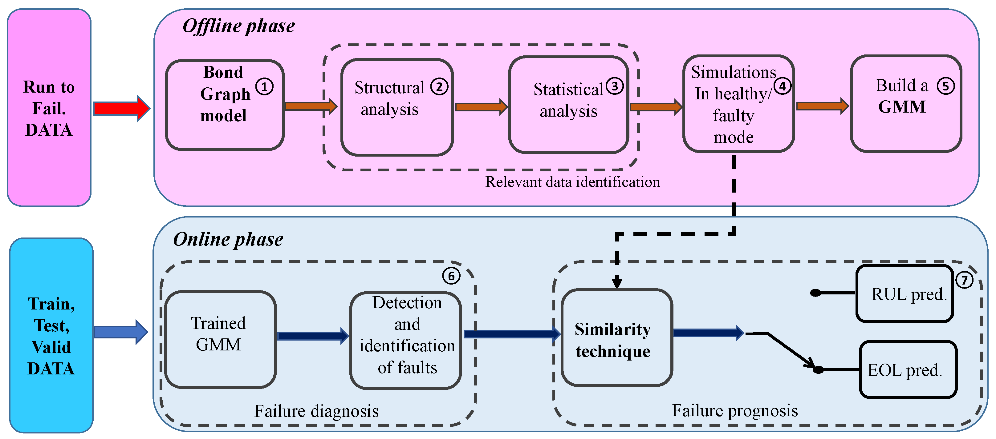
2. Proposed Approach

The presented approach is illustrated in Figure 1 and is composed of two phases: the first phase is devoted to learning and the second to monitoring.

The first phase is performed in five steps (1 to 5) and aims to build the GMM clustering model. Step 1 is devoted to the system modeling using the bond graph approach, the model is then used in step 2 for structural analysis, which results in the identification of sensors providing the failure information. A statistical analysis based on prognosability, monotonicity and trendability metrics is applied in step 3 on the generated dataset to reduce the attribute space to only the most relevant ones in order to avoid redundancy.

Then, faulty and normal operations are simulated in step 4, and data from the selected sensors in step 4 are recorded for a GMM model building in step 5. The second stage of the failure prognosis algorithm is implemented online and is organized in two steps: diagnosis step (step 6) where the GMM learned in the first phase is implemented for fault detection and identification. Finally, in the last step (step 7), the diagnostic information is combined with a similarity algorithm to predict the RUL.

2.1. Offline Phase

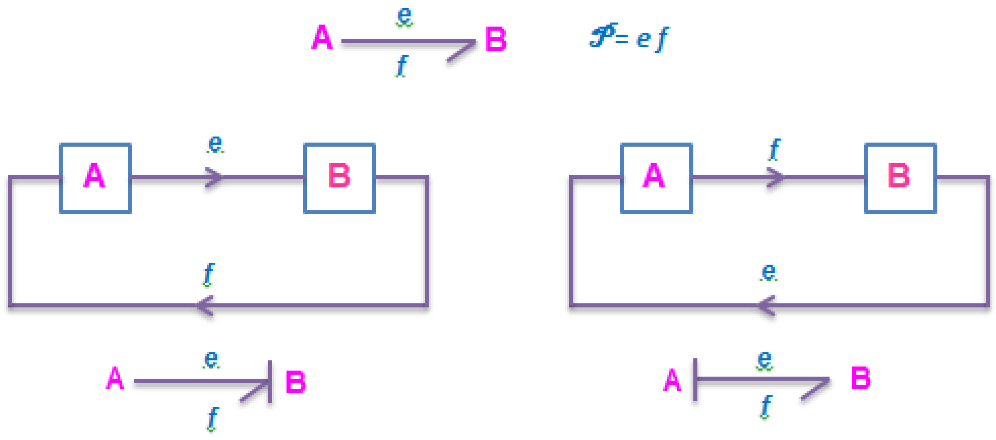
2.1.1. Structural Analysis by Bond Graph

The architecture of the system and the way power is exchanged between elements is represented based on the notion of causality that makes it possible to show explicitly the cause and effect relationships [20]. A causal path in a junction element (0, 1, TF or GY ) is defined as an alternation of bonds and elements (R, C or I ) called nodes such that all nodes have a complete and correct causality, and two bonds of the causal path have opposite causal orientations in the same node. Depending on the causality, the variable crossed is effort or flow. To change this variable it is necessary to pass through a junction element GY, or through a passive element (I, C or R) [21].

By convention, the causal stroke (a short line perpendicular to the bond) is placed near (respectively far from) the element for which the effort (respectively flow) is an input (Figure 2). By defining which of the two variables, effort or flow, is an input, each BG element has two possible causality assignments, and each assignment corresponds to a generic law. A causally completed bond graph may be considered as a compact representation of a block diagram [20,21].

These structural characteristics allow observability of faults by checking whether degradation affecting system elements is observable on existing sensors or not. We take the example of a BG model of an electrical motor with its causal path between control input $MSe:U$ and output sensor $Df:wm$. The causal path relying the input effort $MSe:Um$ and the output angular velocity $Df:Wm$ is illustrated on the model and is given by Figure 3.

$MSe:U_m\to e_1,e_2\to I:L\to f_2,f_4\to GY:K_e\to e_5,e_6\to I:J_m\to f_6,f_7\to Df:W_m$. Thus, any degradation in the value of the elements L or $J_m$ causes a variation in the value observed at the output sensor $Df$. Following this concept, only sensors that carry information on the degradation phenomena will be chosen as inputs for statistical analysis in step 3.

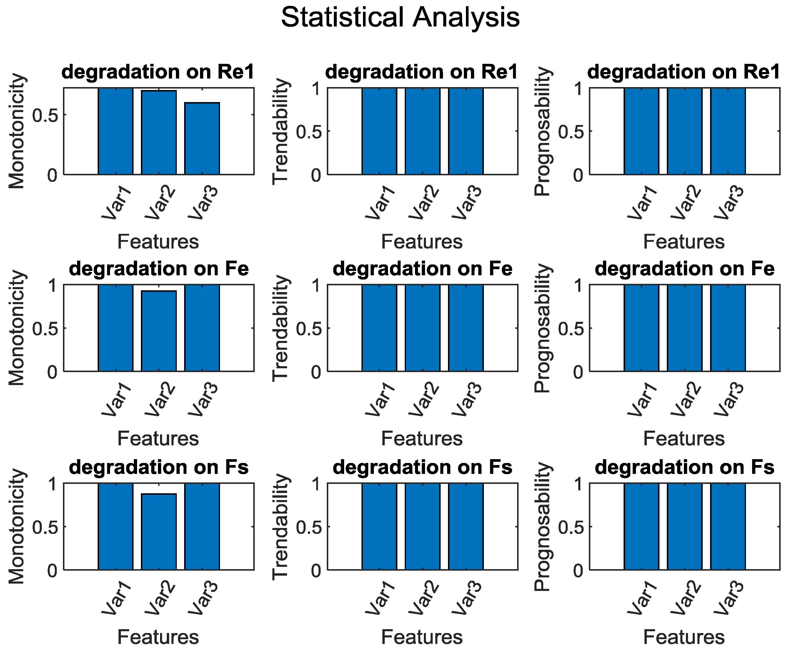
2.1.2. Statistical Analysis

The purpose of this analysis is to confirm the choices of the most relevant data sensors from the previous step using a statistical evaluation metrics (prognosability, monotonicity and trendability). The score is easily interpretable between 0 and 1, where 1 indicates the most satisfactory and 0 the least satisfactory levels of the specific HI property.

Monotonicity: It is related to the irreversibility assumption of degradation phenomena, it indicates the degree to which the parameters of a population are always increasing or decreasing [2].

$$Monotonocity=mean\left|\frac{\#\frac{d}{dx}>0}{N-1}-\frac{\#\frac{d}{dx}<0}{N-1}\right|$$

(1)

Here, $\#\frac{d}{dx}>0$ is the number of sequential data points for witch the second is greater than the first, and $\#\frac{d}{dx}<0$ is the number of sequential data points or the second is less than the first. N : is the number of observations.

Trendability: It indicates the degree, to which the evolution of the HI during the degradation of a population of similar components has the same shape and, thus, can be described by the same functional form [22]. Trendability is given by the smallest absolute correlation:

$$Trendability=min\left(|corrcoe{f}_{ij}\right|),i,j=1,\dots ,N$$

(2)

where $corrcoe{f}_{ij}$ is the linear correlation coefficient between the $i^{th}$ and the $j^{th}$ run-to-failure trajectories.

Prognosability: Is is defined as the standard deviation of the $HI$ value at failure for the available run-to-failure trajectories divided by the average variation of the HI values between the beginning and the end of the trajectories. The obtained value is exponentially weighted to give a metric in the desired 0 to 1 scale:

$$Prognosability=exp\left(\frac{-std\left(H{I}_{fail}\right)}{mean\left|H{I}_{start}-H{I}_{fail}\right|}\right)$$

(3)

where $H{I}_{start}$ and $H{I}_{fail}$ are the $HI$ values at the beginning and the end of the run-to-failure trajectories, respectively; $std\left(H{I}_{fail}\right)$ is the standard deviation of the $HI$ values at the end of the trajectories, $mean|H{I}_{start}|$−$|H{I}_{fail}|$ is the average variation of the $HI$ values between the beginning and the end of the trajectories, respectively [2,22].

2.1.3. Simulations in Normal/Faulty Mode

Once the most relevant sensor are identified; from the previous analysis steps, the block diagram extracted from the BG model and corresponding to the system is used as a simulator to run simulations in normal and faulty mode and therefore to generate a database. Regarding the normal state, data are taken directly from sensors without introducing any degradation on the system. However, for faulty situation, run-to-failure data are simulated by introducing different degradation dynamics with varying parameters on different system components. Therefore, the database contains training vectors representing the system in normal state and several degradations models for each faulty element. The database will then used for training GMM in order to cluster the test vector data.

2.1.4. Gaussian Mixture Model

In recent years, the GMM has been introduced indirectly in the prognostic phase, either by fault diagnosis, which is carried out by degradation data clustering and state division [23,24,25,26], or by assessment the state of degradation by creating HIs [27,28] or even for determining the layers and the number of cells in each layer for LSTM model [29].

GMMs are used in [30] to make the diagnosis by finding to which a GMM, a given testing feature vector is belong by calculating the posteriori probability. In [31,32] GMMs are used for predicting performance degradation; Principal Component Analysis is used to select more sensitive degradation features, then, a degradation index is used to describe the degradation degree of the pump quantitatively is defined combining a GMM and SVR (optimized support vector regression) in [31]. The proposed approach developed in [32] used a GMM based negative log likelihood probability to provide an indicator quantifying the degradation of bearing performance, this study use a locality preserving projections based feature extraction approach to select the most sensitive degradation features.

A GMM is a model that combines several simple Gaussian models M with different weights $W_h$. Each model is characterized by a single density function $N(G,{\mu }_h,\sum h)$ which represents the probability density function (PDF). A GMM can be described by:

$$P\left(G\right)=\sum _{h=1}^M{W}_h{P}_h\left(G\right)=\sum _{h=1}^M{W}_{h}N(G,{\mu }_h,\sum h)$$

(4)

$$N(G,{\mu }_h,\sum h)=\frac{1}{\sqrt{\left(2{\pi }^r\right)|\sum h|}}exp(-\frac{1}{2}{(G-{\mu }_h)}^T)\sum h^{-}1(G-{\mu }_h)$$

(5)

where ${\sum }_{h=1}^M{W}_h=1$, $P_h\left(G\right)=N(G,{\mu }_h,\sum h)$ is the PDF of the $h^{th}$ Gaussian model, ${\mu }_h$ and $\sum h$ are the mean vector and co-variance matrix of the $h^{th}$ Gaussian model, respectively.

From the above definitions, it can be seen that the determination of parameters ($W_h$, ${\mu }_h$ and $\sum h$) greatly affects the performance of the GMM.

In this work, these parameters are chosen in a way that they represent different operating states of the system and therefore training the GMM model considering training vectors clustering.

2.2. Online Phase

2.2.1. Diagnostic Step

Three different GMMs were created considering the three adopted configurations: a GMM with one sensor data, a GMM with two sensors data and a GMM with three sensors data. Each GMM is composed of four elements, which represent different operating states or classes. The first class represents the healthy state of the system while others classes represent different failure states on different element of the system (degradation on element R:$R_{e1}$, degradation on element R:$F_e$ and degradation on element R:$F_s$).

The GMM parameters ($W_h$, ${\mu }_h$ and $\sum h$) are calculated offline for each operating (healthy class and faulty ones) to train the GMM to detect the state of the system and to localize the fault if exists. In the online step, these parameters are calculated and compared to offline parameter values.

2.2.2. Prognosis Step

The similarity technique has been used in different ways in several works such as [33,34,35,36,37] for the prediction of the remaining useful life. In this paper, a similarity model is created for each degradation profile of each GMM component. In the online step, the GMM detects the presence of a fault and identifies it by locating the faulty element and then choose the appropriate model for RUL prediction. The RUL based on the similarity approach is calculated by:

$$RUL=\sum _{i=1}^k{w}_{i}RU{L}_i$$

(6)

The notation $w_i$ stands for the weight assigned to the estimated RUL and depends on the similarity between the test vector and the similarity models created where k is the number of selected neighbours.

3. Application and Experimental Results

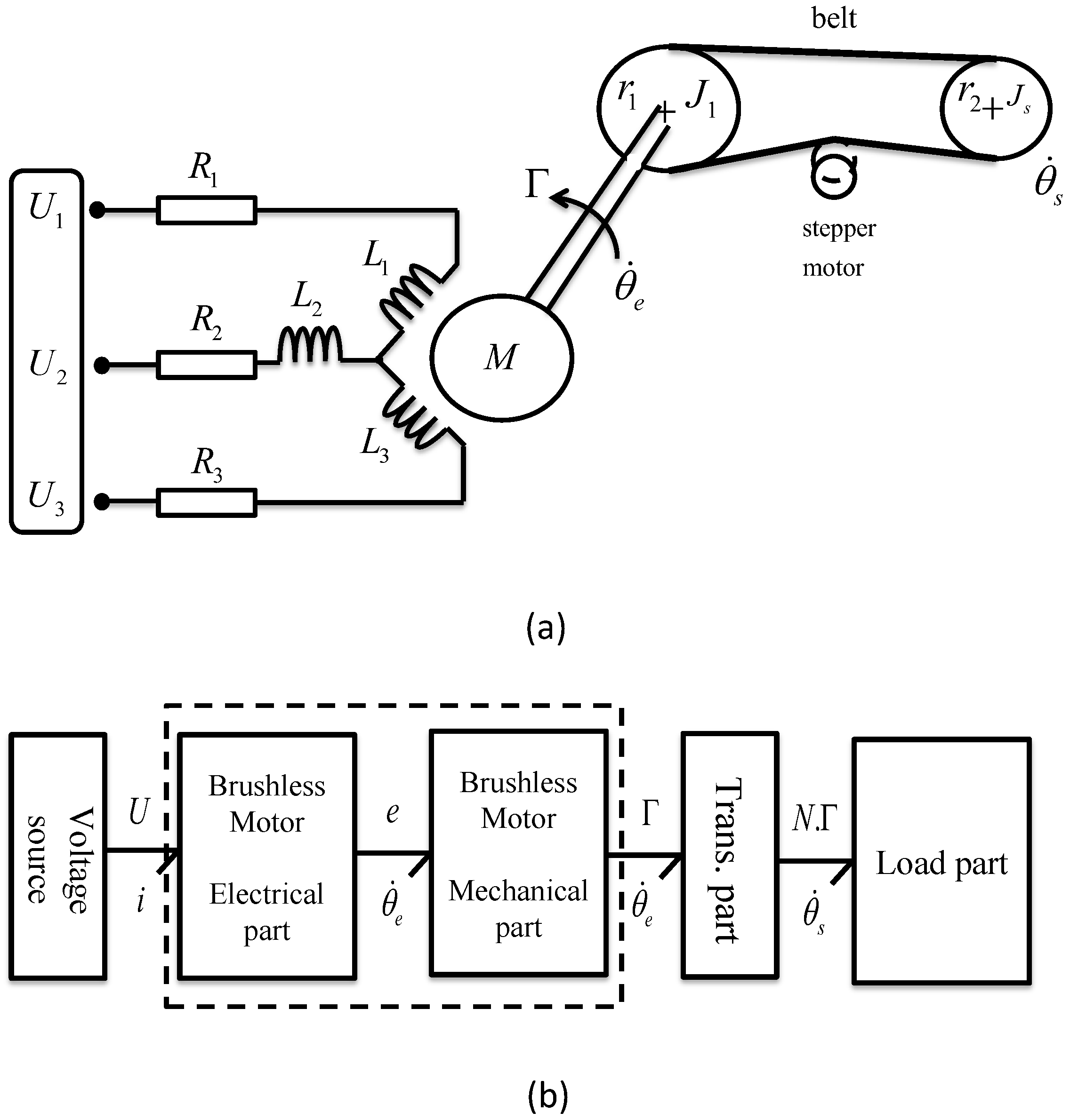
3.1. System Description

The considered mechatronic system Figure 4a used in this work was established and modeled with BG in [38,39]. The overall architecture of the system named word BG is given in Figure 4b where the system is decomposed into three parts: brushless motor part, transmission part and load part:

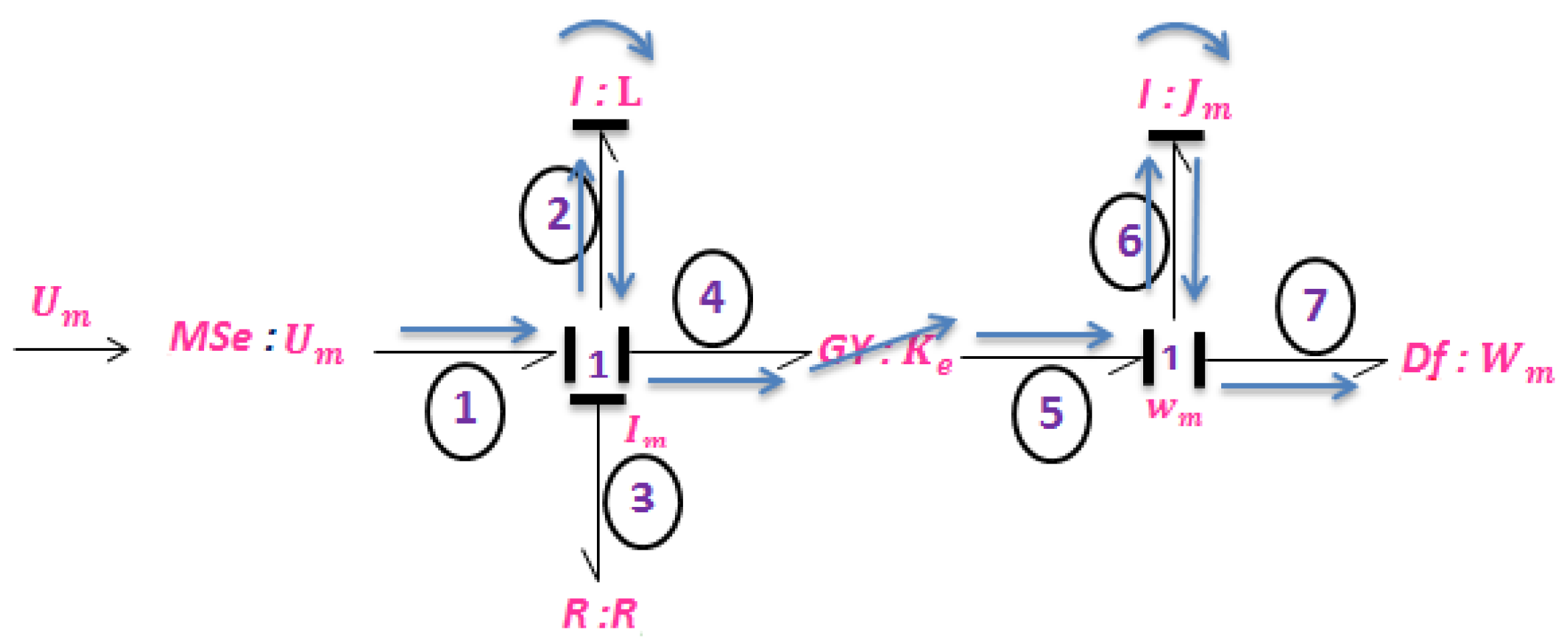
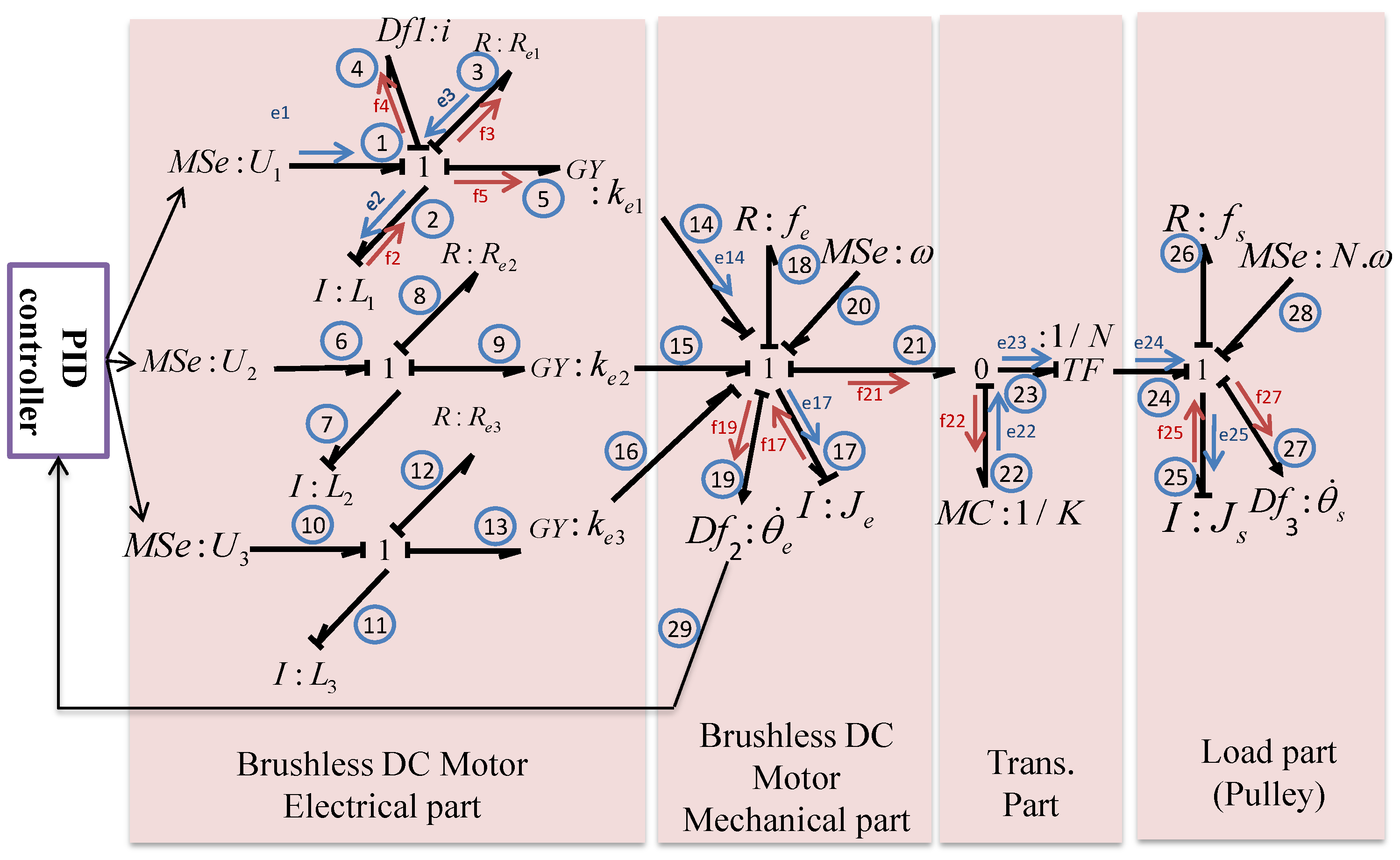
• The brushless motor part is a three phase motor. The electrical part corresponds to three RL circuits. It is composed of an input voltage source $U_j$ with $j=1,\dots 3$, an electrical resistance $R_{ej}$, an inductance $L_j$ and a back electromotive force (EMF) with a constant $k_{ej}$, which is linear to the angular velocity of the rotor. The mechanical part is characterised by the rotor inertia $J_m$, and a viscous friction parameter $f_e$;
• The transmission part concerns the belt which links the mechanical part to the load part. It is characterised by the belt stiffness K and by the transmission reduction constant $N=r2/r1$;
• The load part of the mechatronic system is a pulley that is characterised by its inertia $J_s$ and a viscous friction parameter $f_s$. The instrumentation architecture of this system is composed of the angular position of the rotor ${\theta }_e$ and the angular position of the pulley ${\theta }_s$. Since the position is not a flux variable neither an effort one, the velocities ${\theta }_e$ and ${\theta }_s$ are represented using a $Df$ element on the BG model. They are obtained by differentiating the position information.

The specifications of the mechatronic system are given in

Table 1. Specification of the mechatronic system.

	Nominal Values	Unit	Uncertainties
$f_e$	$0.015$	(N.m.s.rad${}^{-1}$)	$0.02·f_{en}$
$J_e$	$0.01$	(Kg.m${}^2$)	$0.02·J_{en}$
K	$2.01$	(N.m.rad${}^{-1}$)	$0.02·K_n$
N	$1.25$	−	$0.02·N_n$
$f_s$	$0.02$	(N.m.s.rad${}^{-1}$)	$0.02·f_{sn}$
$J_s$	$0.0002$	(Kg.m${}^2$)	$0.02·J_{sn}$

.

3.2. Structural and Statistical Analysis

Three kinds of faults are considered assuming that only one fault can appear at the same time. The fault can affect the elements $R:R_{e1}$, $R:f_e$ or $R:f_s$. The BG model of the mechatronic system with the causal paths between the element: $R:R_{e}1$ and the other three sensors $(D{f}_{1}D{f}_2$ and $D{f}_3)$ is given in Figure 5.

-

A causal path is found between the $R:R_{e1}$ element and the current sensor $\left(D{f}_1\right)$:

$MSe:U_1\stackrel{e_1}{⟶}{1}_1:i\stackrel{e_2}{⟶}I:L_1\underset{f_2}{⟶}{1}_1:i\underset{f_3}{⟶}R:R_{e1}\stackrel{e_3}{⟶}{1}_1:i\stackrel{e_2}{⟶}I:L_1\underset{f_2}{⟶}{1}_1:i\underset{f_4}{⟶}D{f}_1:i$

-

A causal path is found between the $R:R_{e1}$ element and the angular speed of the rotor sensor $\left(D{f}_2\right)$:

$MSe:U_1\stackrel{e_1}{⟶}{1}_1:i\stackrel{e_2}{⟶}I:L_1\underset{f_2}{⟶}{1}_1:i\underset{f_3}{⟶}R:R_{e1}\stackrel{e_3}{⟶}{1}_1:i\stackrel{e_2}{⟶}I:L_1\underset{f_2}{⟶}{1}_1:i\underset{f_5}{⟶}Gy:K_{e1}\stackrel{e_{14}}{⟶}{1}_4:{\theta }_e\stackrel{e_{17}}{⟶}I:J_e\underset{f_{17}}{⟶}{1}_4:{\theta }_e\underset{f_{19}}{⟶}D{f}_2:{\theta }_e$

-

A causal path is found between the $R:R_{e1}$ element and the angular speed of the pulley sensor $\left(D{f}_3\right)$:

$MSe:U_1\stackrel{e_1}{⟶}{1}_1:i\stackrel{e_2}{⟶}I:L_1\underset{f_2}{⟶}{1}_1:i\underset{f_3}{⟶}R:R_{e1}\stackrel{e_3}{⟶}{1}_1:i\stackrel{e_2}{⟶}I:L_1\underset{f_2}{⟶}{1}_1:i\underset{f_5}{⟶}Gy:K_{e1}\stackrel{e_{14}}{⟶}{1}_4:{\theta }_e\stackrel{e_{17}}{⟶}I:J_e\underset{f_{17}}{⟶}{1}_4:{\theta }_e\underset{f_{21}}{⟶}{0}_1:\Gamma \underset{f_{22}}{⟶}Mc:1/K\stackrel{e_{22}}{⟶}{0}_1:\Gamma \stackrel{e_{23}}{⟶}Tf:1/N\stackrel{e_{24}}{⟶}{1}_5:{\theta }_s\stackrel{e_{25}}{⟶}I:J_s\underset{f_{25}}{⟶}{1}_5:{\theta }_s\underset{f_{27}}{⟶}D{f}_3:{\theta }_s$

This means that, in the case of degradation in the performance of the R:$R_{e1}$ element, the degradation is observed from the three sensors $(D{f}_1$, $D{f}_2$ and $D{f}_3)$.

With the same reasoning, different causal paths can be found between the two other elements: $R:f_e$ and $R:f_s$ and the three sensors $D{f}_1$, $D{f}_2$ and $D{f}_3$. In this case study, the data of the three sensors are relevant to make prognosis.

The results of the statistical metrics of monotonicity, trendability and prognosability are elucidated in Figure 6. The results show that the data obtained from the three sensors in the three types of faults are relevant data, which confirms the structural analysis.

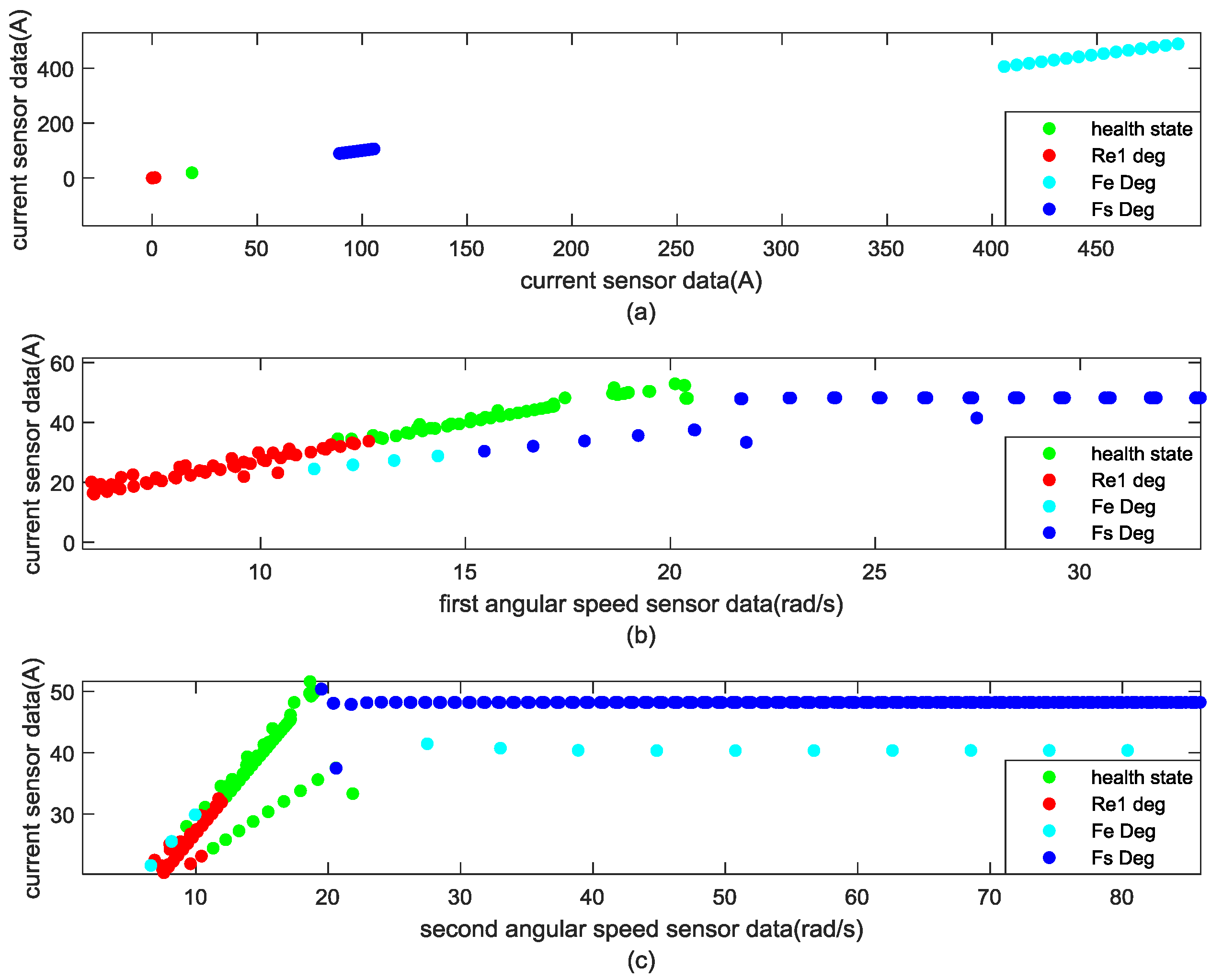
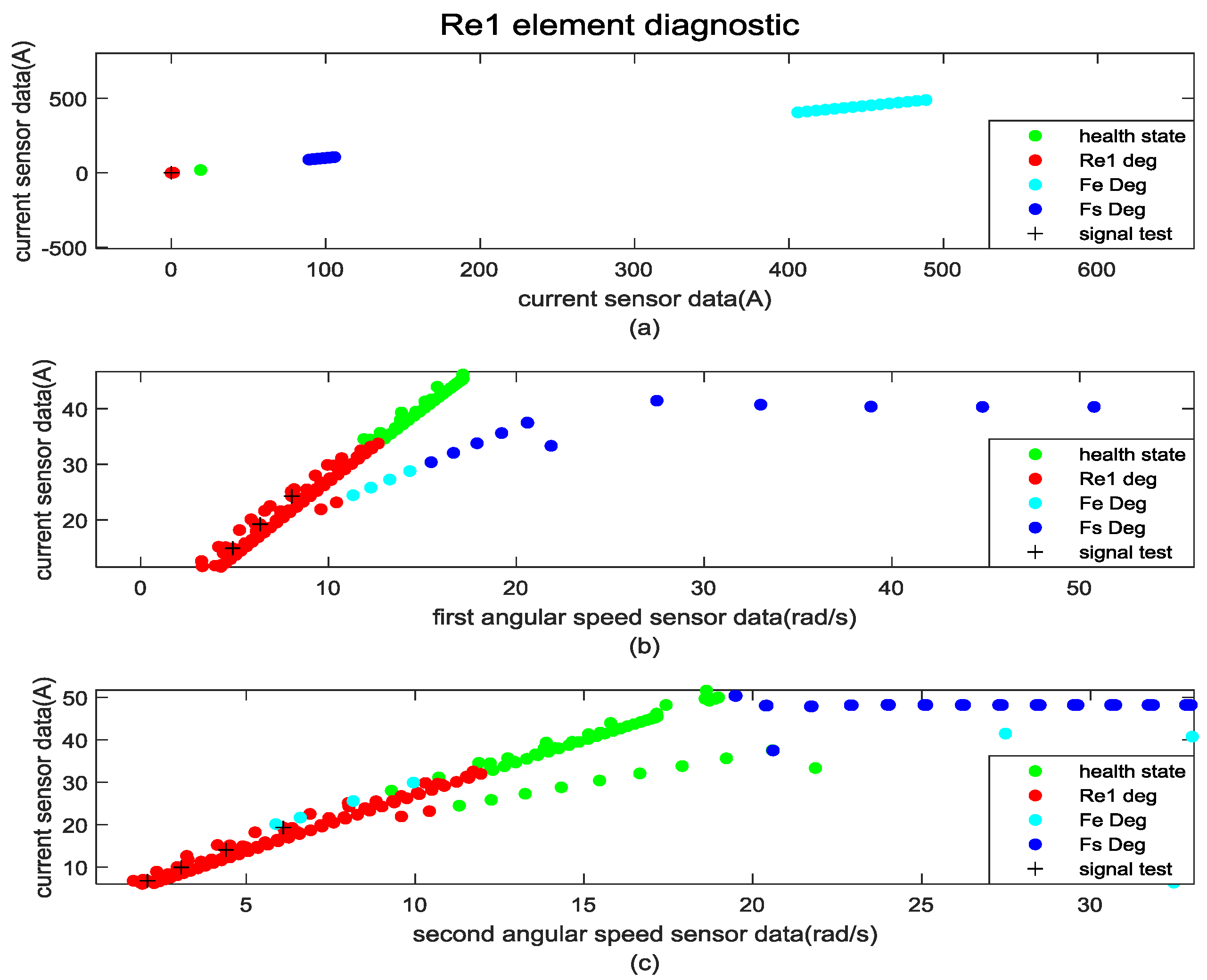
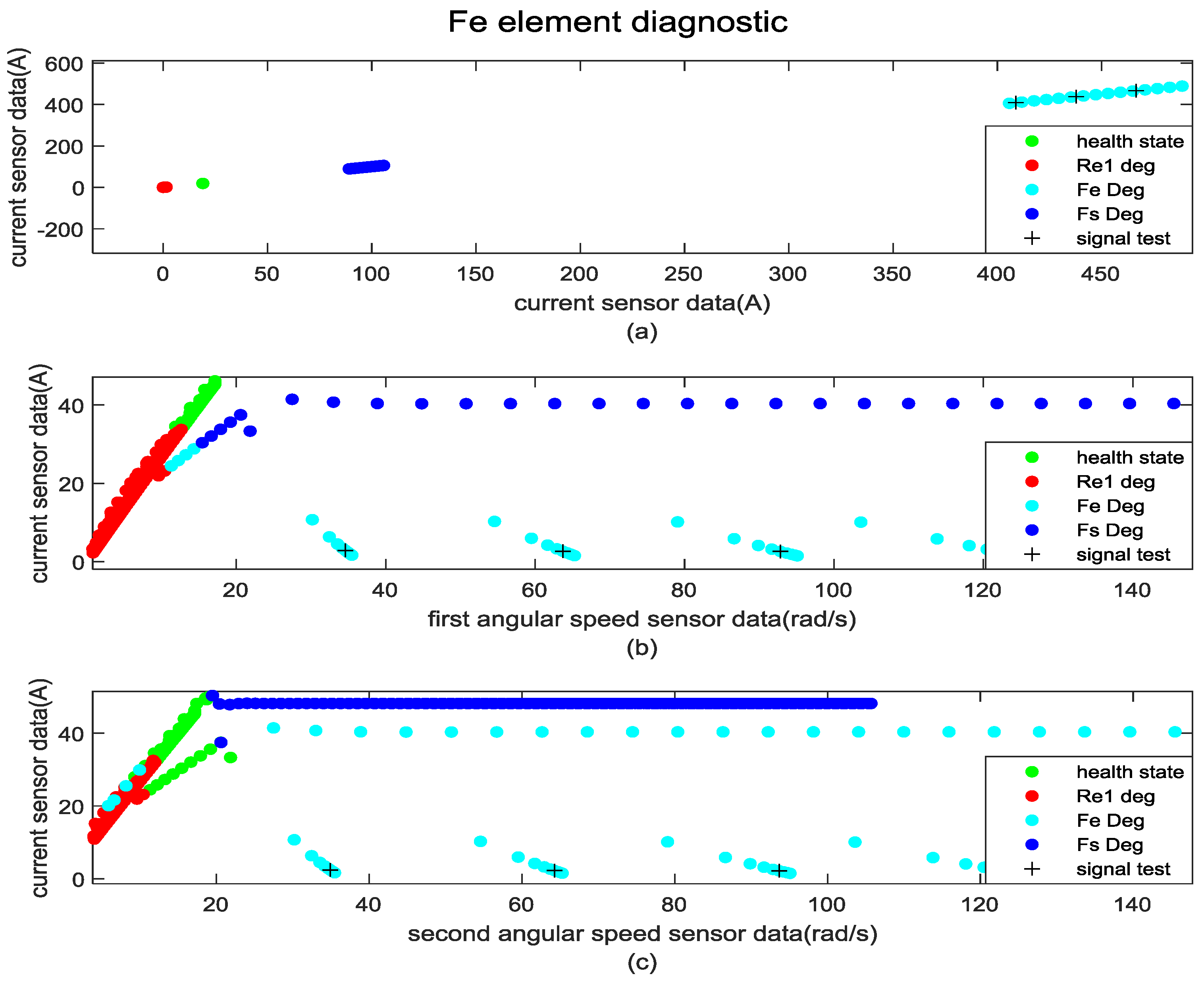
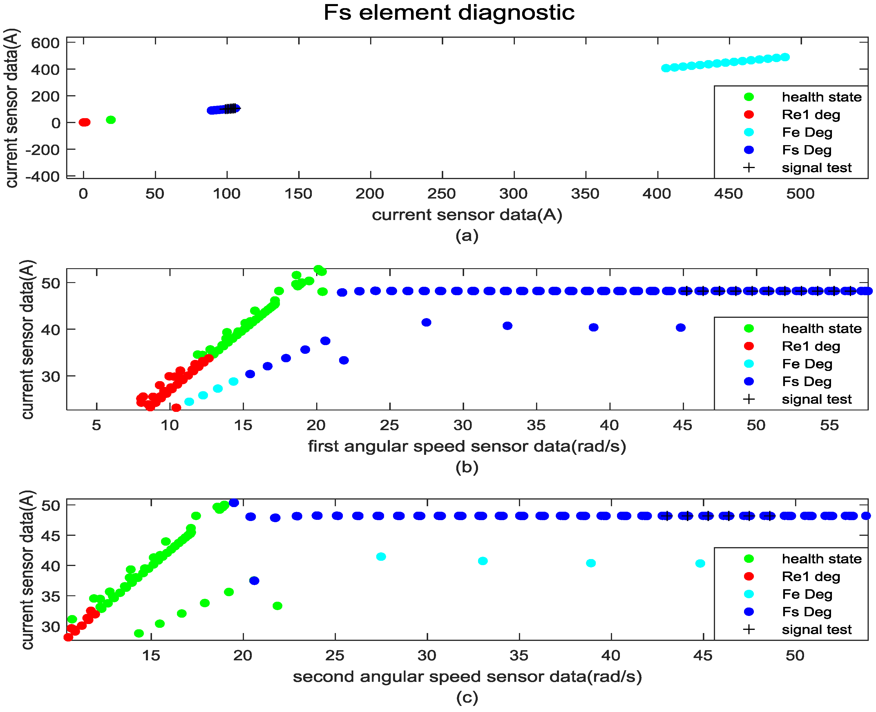
3.3. Clustering and Diagnostic by GMM

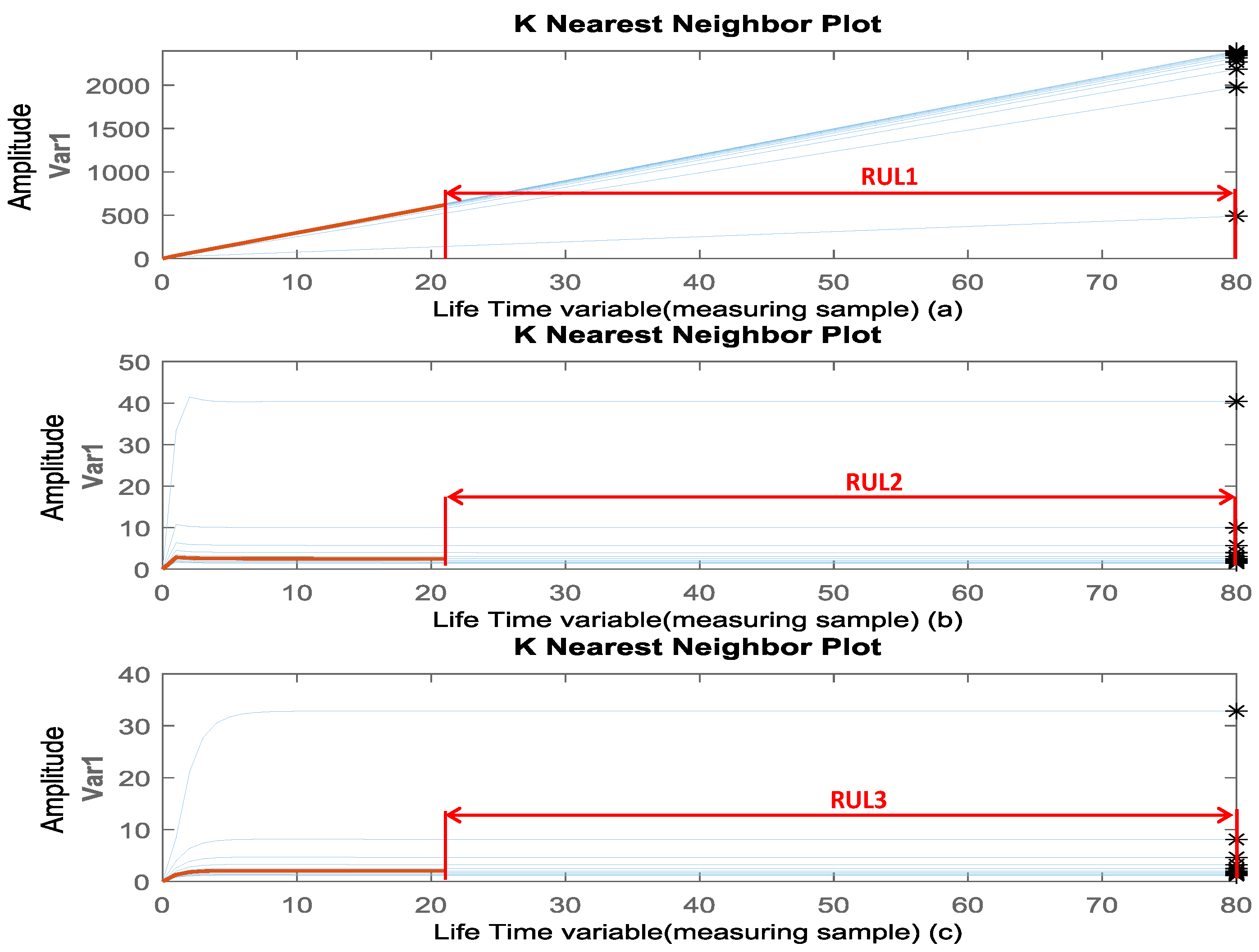
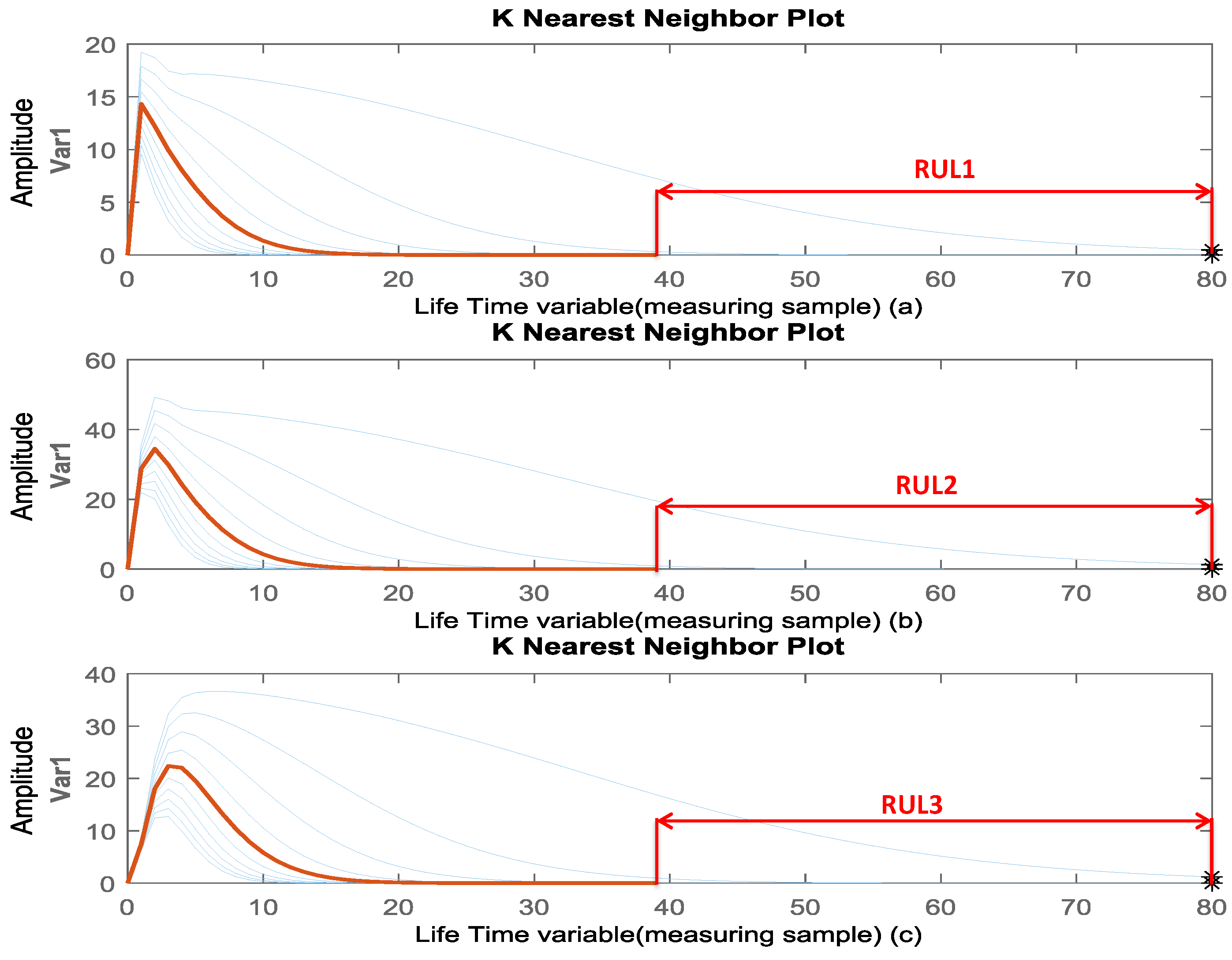
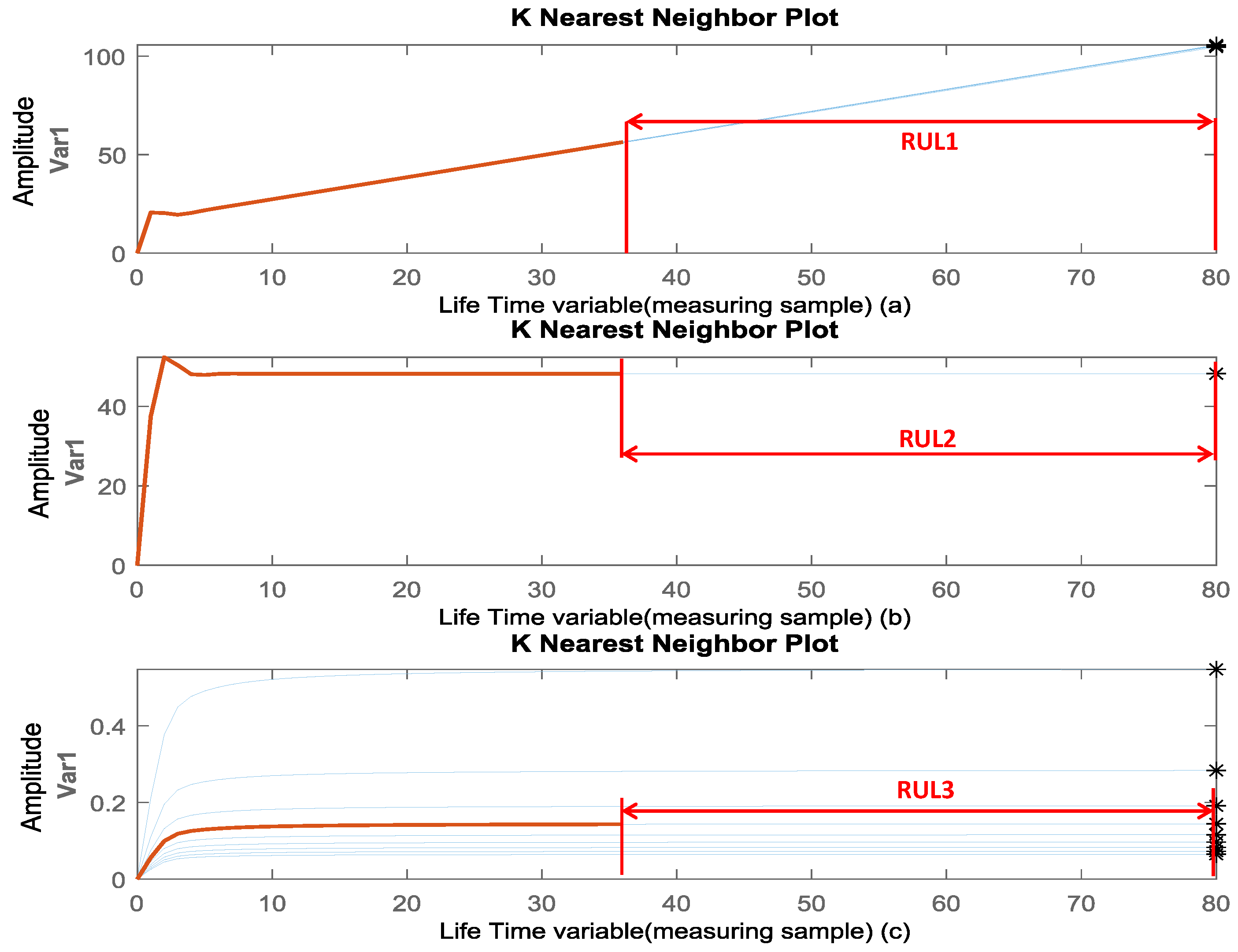
Three different GMMs using the data of one sensor, two sensors and three sensors were created. Knowing that the three sensors have relevant data, the results of clustering presented by Figure 7 indicate that each GMM performs the clustering of the data successfully and represent the different system health states under different types of degradation (an exponential degradation on the element $R_{e1}$, a linear degradation on the two elements $F_e$ and $F_s$) of the system.

In addition, each GMM can detect and locate each fault successfully. Figure 8, Figure 9 and Figure 10 depict the detection and localization of faults under different types of degradation.

3.4. RUL Prediction

After introducing a test vector, which represents degradation on one of the three elements of the system, the RUL prediction of $R_{e1}$, $F_e$ and $F_s$ elements using the three types of data (one sensor, tow sensors and three sensors) are shown in Figure 11, Figure 12 and Figure 13.

Figure 11 indicates that the value of the remaining useful life of element $R_{e1}$ is almost the same in all three cases and is almost “41 measuring simple”, this is after the introduction of a test vector of the length “40 measuring simple”.

Figure 12 shows that the value of the remaining useful life of element $F_e$ is almost “59 measuring simple”, this is after the introduction of a test vector of the length “21 measuring simple” and this is in the three types of data of GMM.

Finally, in Figure 13, the value of the remaining useful life of element $F_s$ is almost “44 measuring simple”, this is after the introduction of a test vector of the length “36 measuring simple”, and this is in the three types of data of GMM.

4. Discussion

In this study, we demonstrate the effectiveness of the proposed hybrid approach based on the BG, GMM and similarity techniques in the prediction of the remaining useful lifetime.

• Indeed, the combination of a physical approach (the BG) for the structural analysis, with a probabilistic tool (GMM) for the diagnosis and a geometrical tool for the prognosis made it possible on the one hand to complete the real measured data by data generated in simulation using the BG model, to take advantage of the power of GMMs in the Gaussian combination for the separation of classes of operation. The geometric aspect of the similarity method, similar to the principle of geolocation, made it possible to predict the RUL without prior knowledge of the degradation profiles.
• In addition, the relevant variables, identified by structural analysis using BG; are affirmed by statistical evaluation metrics.
• For the validation of the proposed method, the similarity technique is used to predict the RUL in three cases: a single sensor, two sensors and three sensors, the results show that the prediction of the RUL is almost the same, so, for the case study, fault diagnosis and failure prognosis can be performed using only one sensor data.

The study is limited to the hypothesis of the appearance of one fault at a time. Therefore, future studies should be considered to study the case of several faults appearing at the same time.

5. Conclusions

In this paper, a method of failure prognosis dealing with dynamic systems is presented. The proposed method investigates all the available knowledge, including physical knowledge through the use of bond graphs for structural analysis and the identification of measures carrying information on the operating state of the system. The statistical properties of the data were investigated by the use of the metrics of monotonicity, trendability and prognosability to find those most relevant for the prognosis. The probabilistic properties of the available data were exploited by the use of GMMs for the classification of faults, and finally the geometric properties of the data available via the similarity method were used for estimating the RUL. The application of the proposed method on a mechatronic system, representative of the systems used in many sectors of industry and transport, showed encouraging results that confirm its effectiveness.

References

1. ISO 13381-1; Condition Monitoring and Diagnostics of Machines—Prognostics—Part 1: General Guidelines. ISO: Geneva, Switzerland, 2015.
2. Djeziri, M.A.; Benmoussa, S.; Zio, E. Review on Health Indices Extraction and Trend Modeling for Remaining Useful Life Estimation. In Artificial Intelligence Techniques for a Scalable Energy Transition; Springer: Berlin/Heidelberg, Germany, 2020; pp. 183–223. [Google Scholar]
3. Park, Y.J.; Fan, S.K.S.; Hsu, C.Y. A review on fault detection and process diagnostics in industrial processes. Processes 2020, 8, 1123. [Google Scholar] [CrossRef]
4. Kordestani, M.; Saif, M.; Orchard, M.E.; Razavi-Far, R.; Khorasani, K. Failure prognosis and applications—A survey of recent literature. IEEE Trans. Reliab. 2019, 70, 728–748. [Google Scholar] [CrossRef]
5. Djeziri, M.; Djedidi, O.; Benmoussa, S.; Bendahan, M.; Seguin, J.L. Failure Prognosis Based on Relevant Measurements Identification and Data-Driven Trend-Modeling: Application to a Fuel Cell System. Processes 2021, 9, 328. [Google Scholar] [CrossRef]
6. Li, N.; Lei, Y.; Yan, T.; Li, N.; Han, T. A Wiener-process-model-based method for remaining useful life prediction considering unit-to-unit variability. IEEE Trans. Ind. Electron. 2018, 66, 2092–2101. [Google Scholar] [CrossRef]
7. Cui, L.; Wang, X.; Wang, H.; Ma, J. Research on remaining useful life prediction of rolling element bearings based on time-varying Kalman filter. IEEE Trans. Instrum. Meas. 2019, 69, 2858–2867. [Google Scholar] [CrossRef]
8. Moulahi, M.H.; Ben Hmida, F. Using extended Kalman filter for failure detection and prognostic of degradation process in feedback control system. Proc. Inst. Mech. Eng. Part I: J. Syst. Control. Eng. 2022, 236, 182–199. [Google Scholar] [CrossRef]
9. Cong, X.; Zhang, C.; Jiang, J.; Zhang, W.; Jiang, Y.; Jia, X. An improved unscented particle filter method for remaining useful life prognostic of Lithium-ion batteries with Li(NiMnCo)O2 cathode with capacity diving. IEEE Access 2020, 8, 58717–58729. [Google Scholar] [CrossRef]
10. Kukurowski, N.; Pazera, M.; Witczak, M. Takagi–Sugeno Observer Design for Remaining Useful Life Estimation of Li-Ion Battery System under Faults. Electronics 2020, 9, 1537. [Google Scholar] [CrossRef]
11. Ekanayake, T.; Dewasurendra, D.; Abeyratne, S.; Ma, L.; Yarlagadda, P. Model-based fault diagnosis and prognosis of dynamic systems: A review. Procedia Manuf. 2019, 30, 435–442. [Google Scholar] [CrossRef]
12. Ahmad, W.; Khan, S.A.; Islam, M.M.; Kim, J.M. A reliable technique for remaining useful life estimation of rolling element bearings using dynamic regression models. Reliab. Eng. Syst. Saf. 2019, 184, 67–76. [Google Scholar] [CrossRef]
13. Zhong, K.; Han, M.; Han, B. Data-driven based fault prognosis for industrial systems: A concise overview. IEEE/CAA J. Autom. Sin. 2019, 7, 330–345. [Google Scholar] [CrossRef]
14. Benmoussa, S.; Djeziri, M.A.; Sanchez, R. Support Vector Machine Classification of Current Data for Fault Diagnosis and Similarity-Based Approach for Failure Prognosis in Wind Turbine Systems. In Artificial Intelligence Techniques for a Scalable Energy Transition; Springer: Berlin/Heidelberg, Germany, 2020; pp. 157–182. [Google Scholar]
15. Motahari-Nezhad, M.; Jafari, S.M. ANFIS system for prognosis of dynamometer high-speed ball bearing based on frequency domain acoustic emission signals. Measurement 2020, 166, 108154. [Google Scholar] [CrossRef]
16. Arunthavanathan, R.; Khan, F.; Ahmed, S.; Imtiaz, S. A deep learning model for process fault prognosis. Process Saf. Environ. Prot. 2021, 154, 467–479. [Google Scholar] [CrossRef]
17. Dong, L.J.; Tang, Z.; Li, X.B.; Chen, Y.C.; Xue, J.C. Discrimination of mining microseismic events and blasts using convolutional neural networks and original waveform. J. Cent. South Univ. 2020, 27, 3078–3089. [Google Scholar] [CrossRef]
18. Tang, S.J.; Yu, C.Q.; Feng, Y.B.; Xie, J.; Gao, Q.H.; Si, X.S. Remaining useful life estimation based on Wiener degradation processes with random failure threshold. J. Cent. South Univ. 2016, 23, 2230–2241. [Google Scholar] [CrossRef]
19. Nor, A.K.M.; Pedapati, S.R.; Muhammad, M.; Leiva, V. Overview of Explainable Artificial Intelligence for Prognostic and Health Management of Industrial Assets Based on Preferred Reporting Items for Systematic Reviews and Meta-Analyses. Sensors 2021, 21, 8020. [Google Scholar] [CrossRef]
20. Dauphin-Tanguy, G. Les bond graphs et leur application en mécatronique. Tech. L’ingénieur. Inform. Ind. 1999, 9 (Suppl. 7222), 1–24. [Google Scholar] [CrossRef]
21. Borutzky, W. Bond Graph Methodology: Development and Analysis of Multidisciplinary Dynamic System Models; Springer Science & Business Media: Berlin/Heidelberg, Germany, 2009. [Google Scholar]
22. Baraldi, P.; Bonfanti, G.; Zio, E. Differential evolution-based multi-objective optimization for the definition of a health indicator for fault diagnostics and prognostics. Mech. Syst. Signal Process. 2018, 102, 382–400. [Google Scholar] [CrossRef]
23. Wang, Z.; Zarader, J.L.; Argentieri, S. A novel aircraft fault diagnosis and prognosis system based on Gaussian mixture models. In Proceedings of the 2012 12th International Conference on Control Automation Robotics & Vision (ICARCV), Guangzhou, China, 5–7 December 2012; IEEE: New Jersey, NJ, USA, 2012; pp. 1794–1799. [Google Scholar]
24. Peng, Y.; Cheng, J.; Liu, Y.; Li, X.; Peng, Z. An adaptive data-driven method for accurate prediction of remaining useful life of rolling bearings. Front. Mech. Eng. 2018, 13, 301–310. [Google Scholar] [CrossRef]
25. Wang, J.; Zhang, L.; Zheng, Y.; Wang, K. Adaptive prognosis of centrifugal pump under variable operating conditions. Mech. Syst. Signal Process. 2019, 131, 576–591. [Google Scholar] [CrossRef]
26. Ma, Y.F.; Jia, X.; Hu, Q.; Bai, H.; Guo, C.; Wang, S. A new state recognition and prognosis method based on a sparse representation feature and the hidden semi-markov model. IEEE Access 2020, 8, 119405–119420. [Google Scholar] [CrossRef]
27. Wang, X.L.; Gu, H.; Xu, L.; Hu, C.; Guo, H. A SVR-based remaining life prediction for rolling element bearings. J. Fail. Anal. Prev. 2015, 15, 548–554. [Google Scholar] [CrossRef]
28. Rai, A.; Upadhyay, S.H. An integrated approach to bearing prognostics based on EEMD-multi feature extraction, Gaussian mixture models and Jensen-Rényi divergence. Appl. Soft Comput. 2018, 71, 36–50. [Google Scholar] [CrossRef]
29. Sayah, M.; Guebli, D.; Noureddine, Z.; Al Masry, Z. Deep LSTM Enhancement for RUL Prediction Using Gaussian Mixture Models. Autom. Control Comput. Sci. 2021, 55, 15–25. [Google Scholar] [CrossRef]
30. Yu, G.; Li, C.; Sun, J. Machine fault diagnosis based on Gaussian mixture model and its application. Int. J. Adv. Manuf. Technol. 2010, 48, 205–212. [Google Scholar] [CrossRef]
31. Lu, C.; Wang, S. Performance Degradation Prediction Based on a Gaussian Mixture Model and Optimized Support Vector Regression for an Aviation Piston Pump. Sensors 2020, 20, 3854. [Google Scholar] [CrossRef]
32. Yu, J. Bearing performance degradation assessment using locality preserving projections and Gaussian mixture models. Mech. Syst. Signal Process. 2011, 25, 2573–2588. [Google Scholar] [CrossRef]
33. Bektas, O.; Jones, J.A.; Sankararaman, S.; Roychoudhury, I.; Goebel, K. A neural network filtering approach for similarity-based remaining useful life estimation. Int. J. Adv. Manuf. Technol. 2019, 101, 87–103. [Google Scholar] [CrossRef] [Green Version]
34. Yu, W.; Kim, I.Y.; Mechefske, C. An improved similarity-based prognostic algorithm for RUL estimation using an RNN autoencoder scheme. Reliab. Eng. Syst. Saf. 2020, 199, 106926. [Google Scholar] [CrossRef]
35. Wang, T.; Yu, J.; Siegel, D.; Lee, J. A similarity-based prognostics approach for remaining useful life estimation of engineered systems. In Proceedings of the 2008 International Conference on Prognostics and Health Management, Denver, CO, USA, 6–9 October 2008; IEEE: Piscataway, NJ, USA, 2008; pp. 1–6. [Google Scholar]
36. Cai, H.; Jia, X.; Feng, J.; Li, W.; Pahren, L.; Lee, J. A similarity based methodology for machine prognostics by using kernel two sample test. ISA Trans. 2020, 103, 112–121. [Google Scholar] [CrossRef]
37. Shu, J.; Xu, Y.; Jin, X.; Han, D.; Xia, T. A Novel Similarity-based Method for Remaining Useful Life Prediction under Multiple Fault Modes. In Proceedings of the 2021 Global Reliability and Prognostics and Health Management (PHM-Nanjing), Nanjing, China, 15–17 October 2021; IEEE: Piscataway, NJ, USA, 2021; pp. 1–7. [Google Scholar]
38. Benmoussa, S.; Djeziri, M.A. Remaining useful life estimation without needing for prior knowledge of the degradation features. IET Sci. Meas. Technol. 2017, 11, 1071–1078. [Google Scholar] [CrossRef]
39. Benmoussa, S.; Djeziri, M. Experimental Application on a Mechanical Transmission System of Integrated Fault Diagnosis and Fault Prognosis method. IFAC-PapersOnLine 2018, 51, 1016–1023. [Google Scholar] [CrossRef]
Figure 1. A schema of the presented approach.
Processes 10 00435 g001
Figure 2. Equivalence between causality on a bond graph and a block diagram.
Processes 10 00435 g002
Figure 3. BG model of an electrical motor with its causal path.
Processes 10 00435 g003
Figure 4. (a) Considered mechatronic system, (b) Corresponding word BG model.
Processes 10 00435 g004
Figure 5. Causal bond graph model of the considered mechatronic system.
Processes 10 00435 g005
Figure 6. Statistical analysis considering the three types of faults.
Processes 10 00435 g006
Figure 7. GMM for data clustering using: (a) D f 1 sensor, (b) D f 1 and D f 2 sensors and (c) D f 1 and D f 3 sensors.
Processes 10 00435 g007
Figure 8. Diagnosis results of fault on R: R e 1 element using: (a) D f 1 sensor, (b) D f 1 and D f 2 sensors and (c) D f 1 , D f 2 and D f 3 sensors.
Processes 10 00435 g008
Figure 9. Diagnosis results of fault on R: F e element using: (a) D f 1 sensor, (b) D f 1 and D f 2 sensors and (c) D f 1 , D f 2 and D f 3 sensors.
Processes 10 00435 g009
Figure 10. Diagnosis results of fault on R: F s element using: (a) D f 1 sensor, (b) D f 1 and D f 2 sensors and (c) D f 1 , D f 2 and D f 3 sensors.
Processes 10 00435 g010
Figure 11. RUL prediction of degradation on R: R e 1 using: (a) D f 1 sensor, (b) D f 1 and D f 2 sensors and (c) D f 1 , D f 2 and D f 3 sensors.
Processes 10 00435 g011
Figure 12. RUL prediction of degradation on R: F e using: (a) D f 1 sensor, (b) D f 1 and D f 2 sensors and (c) D f 1 , D f 2 and D f 3 sensors.
Processes 10 00435 g012
Figure 13. RUL prediction of degradation on R: F s 1 using: (a) D f 1 sensor, (b) D f 1 and D f 2 sensors and (c) D f 1 , D f 2 and D f 3 sensors.
Processes 10 00435 g013