
Mapping Uncertainties of Soft-Sensors Based on Deep Feedforward Neural Networks through a Novel Monte Carlo Uncertainties Training Process

 , ,
, ,  , , and
Abstract
:1. Introduction
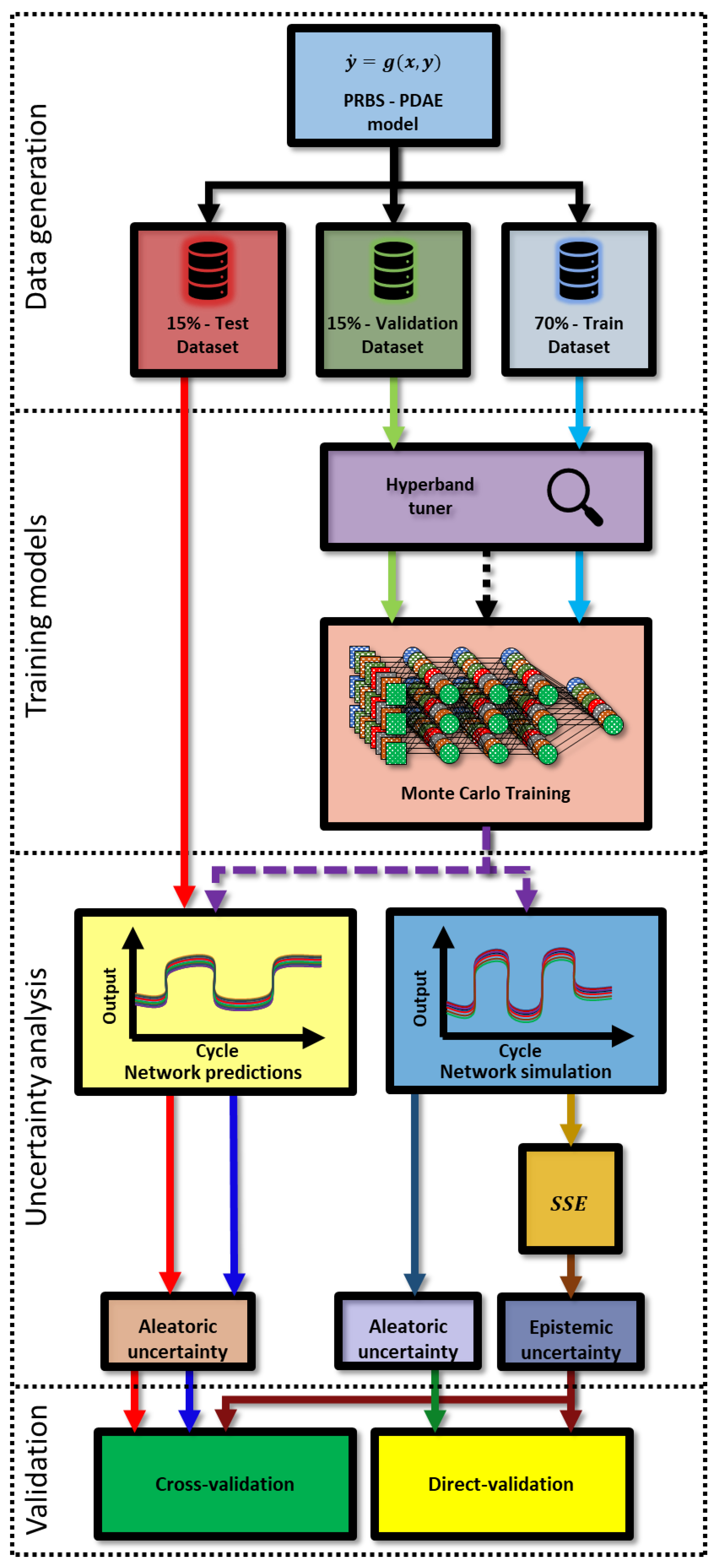
2. Methodology
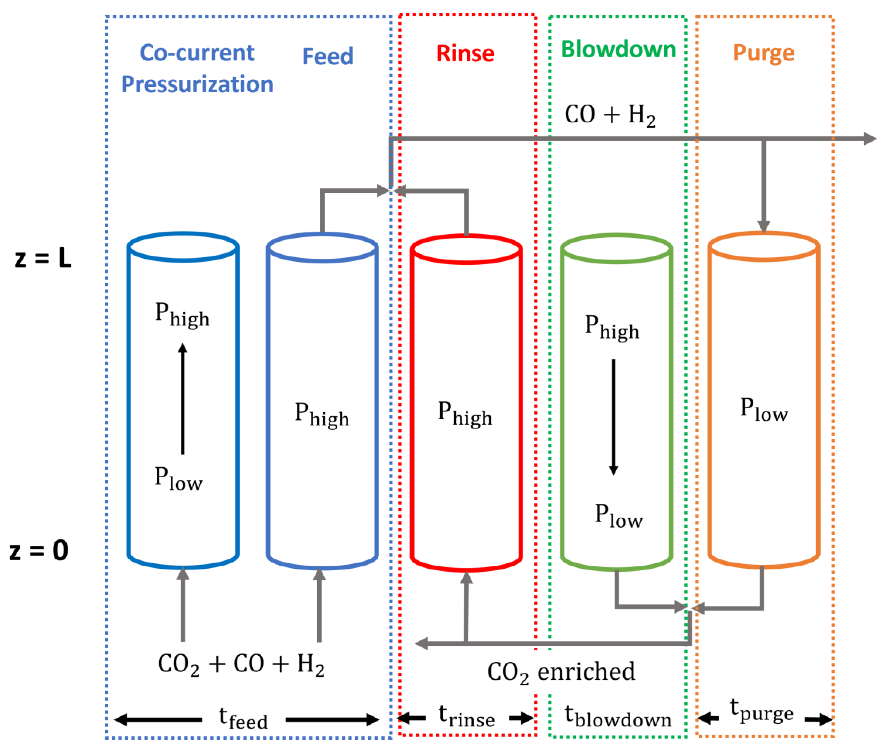
3. Case Study
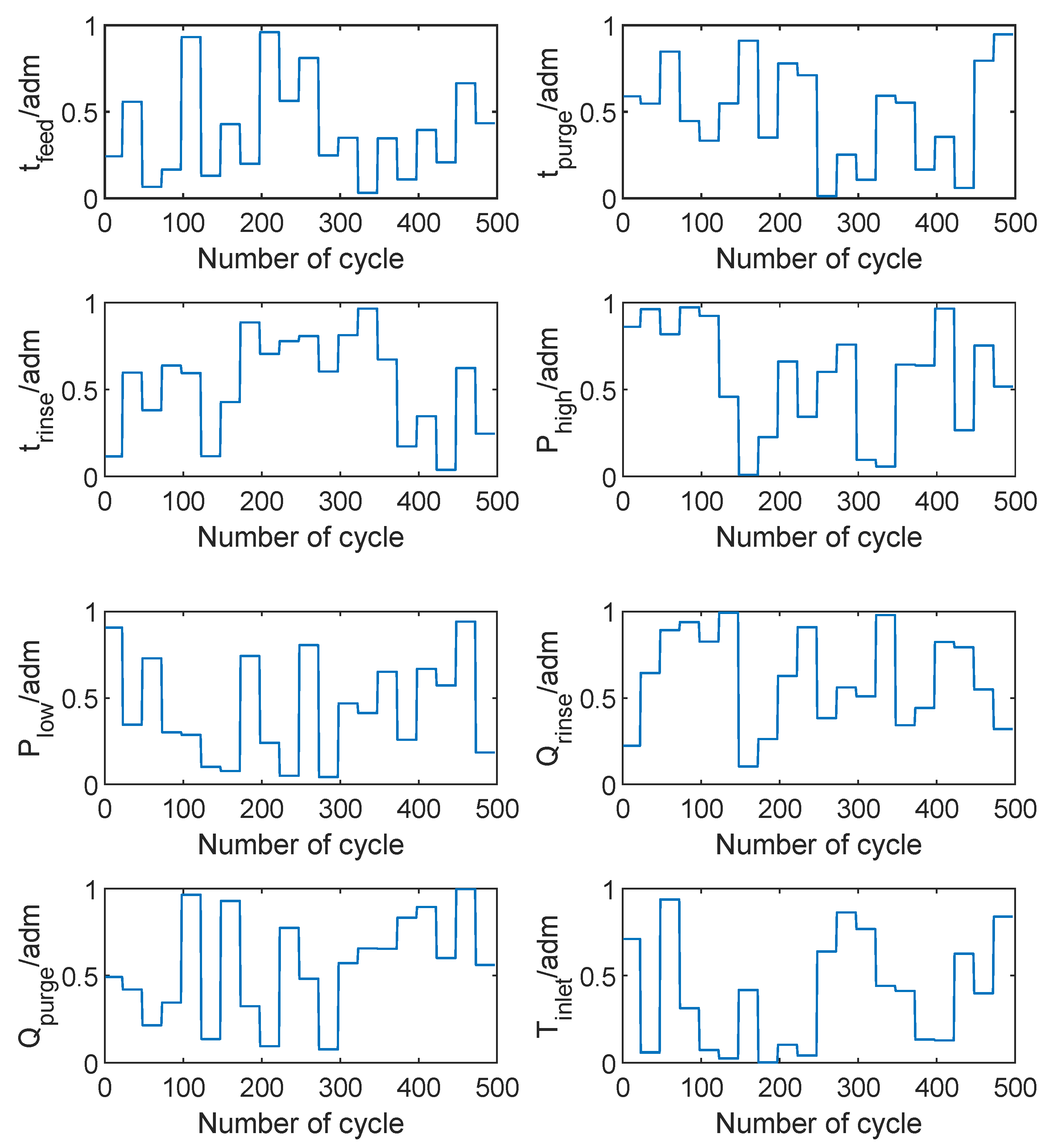
3.1. Data Acquisition
3.2. Predictor and Data Structure
3.3. Hyperparameter Tuning—Hyperband
3.4. Monte Carlo Training
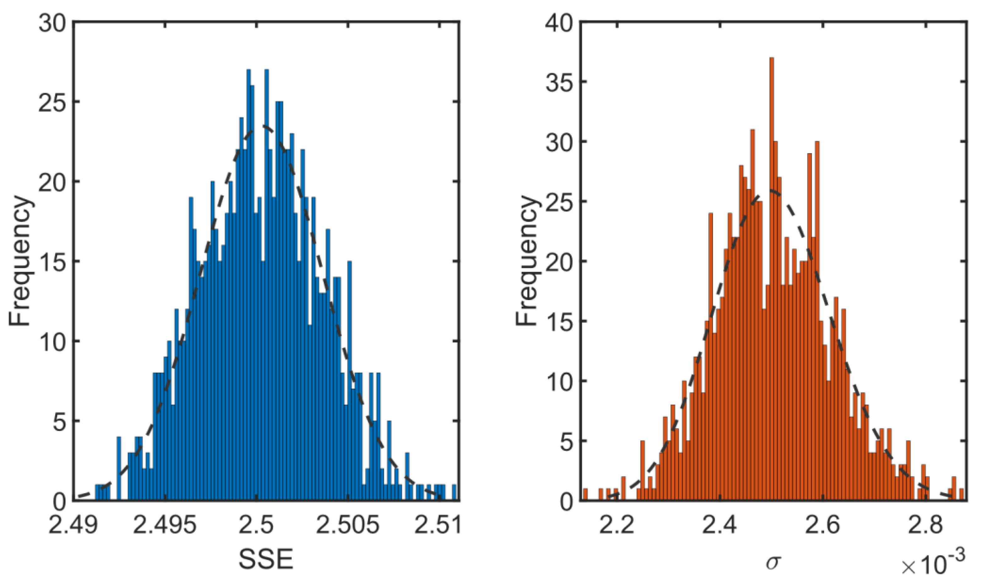
3.5. Uncertainty Analysis
4. Conclusions
Author Contributions
Funding
Conflicts of Interest
References
- Dias, T.; Oliveira, R.; Saraiva, P.; Reis, M.S. Predictive analytics in the petrochemical industry: Research Octane Number (RON) forecasting and analysis in an industrial catalytic reforming unit. Comput. Chem. Eng. 2020, 139, 106912. [Google Scholar] [CrossRef]
- Esme, E.; Karlik, B. Fuzzy c-means based support vector machines classifier for perfume recognition. Appl. Soft Comput. 2016, 46, 452–458. [Google Scholar] [CrossRef]
- Kamat, S.; Madhavan, K. Developing ANN based Virtual/Soft Sensors for Industrial Problems. IFAC-PapersOnLine 2016, 49, 100–105. [Google Scholar] [CrossRef]
- Nogueira, I.; Fontes, C.; Sartori, I.; Pontes, K.; Embiruçu, M. A model-based approach to quality monitoring of a polymerization process without online measurement of product specifications. Comput. Ind. Eng. 2017, 106, 123–136. [Google Scholar] [CrossRef]
- Nogueira, I.B.R.; Ribeiro, A.M.; Requião, R.; Pontes, K.V.; Koivisto, H.; Rodrigues, A.E.; Loureiro, J.M. A quasi-virtual online analyser based on an artificial neural networks and offline measurements to predict purities of raffinate/extract in simulated moving bed processes. Appl. Soft Comput. 2018, 67, 29–47. [Google Scholar] [CrossRef]
- Capriglione, D.; Carratù, M.; Liguori, C.; Paciello, V.; Sommella, P. A soft stroke sensor for motorcycle rear suspension. Meas. J. Int. Meas. Confed. 2017, 106, 46–52. [Google Scholar] [CrossRef]
- Wieder, O.; Kohlbacher, S.; Kuenemann, M.; Garon, A.; Ducrot, P.; Seidel, T.; Langer, T. A compact review of molecular property prediction with graph neural networks. Drug Discov. Today Technol. 2020, 37, 1–12. [Google Scholar] [CrossRef] [PubMed]
- Ren, L.; Xu, B.; Lin, H.; Liu, X.; Yang, L. Sarcasm Detection with Sentiment Semantics Enhanced Multi-level Memory Network. Neurocomputing 2020, 401, 320–326. [Google Scholar] [CrossRef]
- Martins, M.A.F.; Rodrigues, A.E.; Loureiro, J.M.; Ribeiro, A.M.; Nogueira, I.B.R. Artificial Intelligence-oriented economic non-linear model predictive control applied to a pressure swing adsorption unit: Syngas purification as a case study. Sep. Purif. Technol. 2021, 276, 119333. [Google Scholar] [CrossRef]
- Oliveira, L.M.C.; Koivisto, H.; Iwakiri, I.G.I.; Loureiro, J.M.; Ribeiro, A.M.; Nogueira, I.B.R. Modelling of a pressure swing adsorption unit by deep learning and artificial Intelligence tools. Chem. Eng. Sci. 2020, 224, 115801. [Google Scholar] [CrossRef]
- Lee, M.; Bae, J.; Kim, S.B. Uncertainty-aware soft sensor using Bayesian recurrent neural networks. Adv. Eng. Inform. 2021, 50, 101434. [Google Scholar] [CrossRef]
- BIPM; IEC; IFCC; ILAC; ISO; IUPAC; IUPAP; OIML. Evaluation of Measurement Data—Guide To The Expression Of Uncertainty In Measurement; Bureau International des Poids et Measures: France, Paris, 2008. [Google Scholar]
- Rebello, C.M.; Marrocos, P.H.; Costa, E.A.; Santana, V.V.; Rodrigues, A.E.; Ribeiro, A.M.; Nogueira, I.B.R. Machine Learning-Based Dynamic Modeling for Process Engineering Applications: A Guideline for Simulation and Prediction from Perceptron to Deep Learning. Processes 2022, 10, 250. [Google Scholar] [CrossRef]
- Gal, Y.; Ghahramani, Z. Dropout as a Bayesian Approximation: Representing Model Uncertainty in Deep Learning. arXiv 2015, arXiv:1506.02142. [Google Scholar]
- Abdar, M.; Pourpanah, F.; Hussain, S.; Rezazadegan, D.; Liu, L.; Ghavamzadeh, M.; Fieguth, P.; Cao, X.; Khosravi, A.; Acharya, U.R.; et al. A review of uncertainty quantification in deep learning: Techniques, applications and challenges. Inf. Fusion. 2021, 76, 243–297. [Google Scholar] [CrossRef]
- Torgashov, A.; Zmeu, K. Identification of Nonlinear Soft Sensor Models of Industrial Distillation Process under Uncertainty. IFAC-PapersOnLine 2015, 48, 45–50. [Google Scholar] [CrossRef]
- Tang, Q.; Li, D.; Xi, Y. A new active learning strategy for soft sensor modeling based on feature reconstruction and uncertainty evaluation, Chemom. Intell. Lab. Syst. 2018, 172, 43–51. [Google Scholar] [CrossRef]
- da Silva, F.A.; Silva, J.A.; Rodrigues, A.E. A General Package for the Simulation of Cyclic Adsorption Processes. Adsorption 1999, 5, 229–244. [Google Scholar] [CrossRef]
- Regufe, J.; Tamajon, J.; Ribeiro, A.M.; Ferreira, A.F.P.; Lee, U.; Hwang, Y.K.; Chang, J.; Serre, C.; Loureiro, J.M.; Rodrigues, A.E. Syngas Purification by Porous Amino- Functionalized Titanium Terephthalate MIL-125. Energy Fuel. 2015, 29, 4654–4664. [Google Scholar] [CrossRef]
- O’Malley, T.; Bursztein, E.; Long, J.; Chollet, F.; Jin, H.; Invernizzi, L.; de Marmiesse, G.; Fu, Y.; Podivìn, J.; Schäfer, F. KerasTuner. 2019. Available online: https://github.com/keras-team/keras-tuner (accessed on 1 December 2021).
- Ben-Mansour, R.; Habib, M.A.; Bamidele, O.E.; Basha, M.; Qasem, N.A.A.; Peedikakkal, A.; Laoui, T.; Ali, M. Carbon capture by physical adsorption: Materials, experimental investigations and numerical modeling and simulations–review. Appl. Energy. 2016, 161, 225–255. [Google Scholar] [CrossRef]
- Capra, F.; Gazzani, M.; Joss, L.; Mazzotti, M.; Martelli, E. MO-MCS, a Derivative-Free Algorithm for the Multiobjective Optimization of Adsorption Processes. Ind. Eng. Chem. Res. 2018, 57, 9977–9993. [Google Scholar] [CrossRef]
- Siqueira, R.M.; Freitas, G.R.; Peixoto, H.R.; Nascimento, J.F.d.; Musse, A.P.S.; Torres, A.E.B.; Azevedo, D.C.S.; Bastos-Neto, M. Carbon Dioxide Capture by Pressure Swing Adsorption. Energy Procedia. 2017, 114, 2182–2192. [Google Scholar] [CrossRef]
- Subraveti, S.G.; Li, Z.; Prasad, V.; Rajendran, A. Machine Learning-Based Multiobjective Optimization of Pressure Swing Adsorption. Ind. Eng. Chem. Res. 2019, 58, 20412–20422. [Google Scholar] [CrossRef]
- Nogueira, I.B.R.; Martins, M.A.F.; Regufe, M.J.; Rodrigues, A.E.; Loureiro, J.M.; Ribeiro, A.M. Big Data-Based Optimization of a Pressure Swing Adsorption Unit for Syngas Purification: On Mapping Uncertainties from a Metaheuristic Technique. Ind. Eng. Chem. Res. 2020, 59, 14037–14047. [Google Scholar] [CrossRef]
- Li, L.; Jamieson, K.; DeSalvo, G.; Rostamizadeh, A.; Talwalkar, A. Hyperband: A Novel Bandit-Based Approach to Hyperparameter Optimization. J. Mach. Learn. Res. 2016, 18, 1–52. [Google Scholar]
- Marrocos, P.H.; Iwakiri, I.G.I.; Martins, M.A.F.; Rodrigues, A.E.; Joureiro, A.; Ribeiro, I.B.R. A long short-term memory based Quasi-Virtual Analyzer for dynamic real-time soft sensing of a Simulated Moving Bed unit. Appl. Soft Comput. 2022, 116, 108318. [Google Scholar] [CrossRef]
- Santana, V.V.; Martins, M.A.F.; Loureiro, J.M.; Ribeiro, A.M.; Rodrigues, A.E.; Nogueira, I.B.R. Optimal fragrances formulation using a deep learning neural network architecture: A novel systematic approach. Comput. Chem. Eng. 2021, 150, 107344. [Google Scholar] [CrossRef]
- Schweidtmann, A.M.; Esche, E.; Fischer, A.; Kloft, M.; Repke, J.U.; Sager, S.; Mitsos, A. Machine Learning in Chemical Engineering: A Perspective. Chem. Ing. Technik. 2021, 93, 2029–2039. [Google Scholar] [CrossRef]
- BIPM; IEC; IFCC; ILAC; ISO; IUPAC; IUPAP; OIML. Evaluation of measurement data–Supplement 1 to the “Guide to the expression of uncertainty in measurement”—Propagation of distributions using a Monte Carlo method, Evaluation. JCGM 2008, 101, 90. [Google Scholar]
- Haario, H.; Laine, M.; Mira, A.; Saksman, E. DRAM: Efficient adaptive MCMC. Stat. Comput. 2006, 16, 339–354. [Google Scholar] [CrossRef]
- Haario, H.; Saksman, E.; Tamminen, J. An adaptive Metropolis algorithm. Bernoulli 2001, 7, 223–242. [Google Scholar] [CrossRef] [Green Version]
- Gelman, A.; Carlin, J.B.; Stern, H.S.; Dunson, D.B.; Vehtari, A.; Rubin, D.B. Bayesian Data Analysis (with Errors Fixed as of 13 February 2020), 3rd ed.; Chapman and Hall/CRC: Boca Raton, FL, USA, 2020; Volume 2013, p. 677. [Google Scholar]


| tfeed/(s) | tpurge/(s) | trinse/(s) | Phigh/(bar) | Plow/(bar) | Qrinse/(SLPM) | Qpurge/(SLPM) | Tinlet/(K) | |
|---|---|---|---|---|---|---|---|---|
| Minimum | 380 | 80 | 187 | 3.4 | 0.55 | 0.425 | 0.225 | 304 |
| Maximum | 680 | 110 | 253 | 5.0 | 1.10 | 0.575 | 0.345 | 350 |
| Hyperparameters of DFNN | ||
|---|---|---|
| Hyperspace | Results | |
| Initial learning rate | {1 × 10⁻⁴, 1 × 10⁻³, 1 × 10⁻¹} | {1 × 10⁻²} |
| Number of dense layers | {1, 2, 3, 4, 5} | {3} |
| Recurrent layer type | - | |
| Number of neurons in the recurrent layers | 50 to 180, every 20 | 90 |
| Activation function in the recurrent layers | {relu, tanh} | {relu} |
| RNN | FNN | |
|---|---|---|
| Initial learning rate | {} | {} |
| Number of layers | {5} | {1} |
| Number of neurons of the layers | {100, 60, 100, 40, 60} | {150} |
| Activation function of the layers | {tanh, tanh, relu, relu, tanh} | {relu} |
| Network | MAE | MSE |
|---|---|---|
| RNN | 0.5688 | 0.3621 |
| FNN | 0.2209 | 0.0796 |
| DFNN | 0.1746 | 0.0587 |
Publisher’s Note: MDPI stays neutral with regard to jurisdictional claims in published maps and institutional affiliations. |
© 2022 by the authors. Licensee MDPI, Basel, Switzerland. This article is an open access article distributed under the terms and conditions of the Creative Commons Attribution (CC BY) license (https://creativecommons.org/licenses/by/4.0/).
Share and Cite
Costa, E.A.; Rebello, C.M.; Santana, V.V.; Rodrigues, A.E.; Ribeiro, A.M.; Schnitman, L.; Nogueira, I.B.R. Mapping Uncertainties of Soft-Sensors Based on Deep Feedforward Neural Networks through a Novel Monte Carlo Uncertainties Training Process. Processes 2022, 10, 409. https://doi.org/10.3390/pr10020409
Costa EA, Rebello CM, Santana VV, Rodrigues AE, Ribeiro AM, Schnitman L, Nogueira IBR. Mapping Uncertainties of Soft-Sensors Based on Deep Feedforward Neural Networks through a Novel Monte Carlo Uncertainties Training Process. Processes. 2022; 10(2):409. https://doi.org/10.3390/pr10020409
Chicago/Turabian StyleCosta, Erbet A., Carine M. Rebello, Vinicius V. Santana, Alírio E. Rodrigues, Ana M. Ribeiro, Leizer Schnitman, and Idelfonso B. R. Nogueira. 2022. "Mapping Uncertainties of Soft-Sensors Based on Deep Feedforward Neural Networks through a Novel Monte Carlo Uncertainties Training Process" Processes 10, no. 2: 409. https://doi.org/10.3390/pr10020409
APA StyleCosta, E. A., Rebello, C. M., Santana, V. V., Rodrigues, A. E., Ribeiro, A. M., Schnitman, L., & Nogueira, I. B. R. (2022). Mapping Uncertainties of Soft-Sensors Based on Deep Feedforward Neural Networks through a Novel Monte Carlo Uncertainties Training Process. Processes, 10(2), 409. https://doi.org/10.3390/pr10020409