Abstract
Oil and gas pipelines are lifelines for a country’s economic survival. As a result, they must be closely monitored to maximize their performance and avoid product losses in the transportation of petroleum products. However, they can collapse, resulting in dangerous repercussions, financial losses, and environmental consequences. Therefore, assessing the pipe condition and quality would be of great significance. Pipeline safety is ensured using a variety of inspection techniques, despite being time-consuming and expensive. To address these inefficiencies, this study develops a model that anticipates sources of failure in oil pipelines based on specific factors related to pipe diameter and age, service (transported product), facility type, and land use. The model is developed using a multilayer perceptron (MLP) neural network, radial basis function (RBF) neural network, and multinomial logistic (MNL) regression based on historical data from pipeline incidents. With an average validity of 84% for the MLP, 85% for the RBF, and 81% for the MNL, the models can forecast pipeline failures owing to corrosion and third-party activities. The developed model can help pipeline operators and decision makers detect different failure sources in pipelines and prioritize the required maintenance and replacement actions.
1. Introduction
Pipelines, which are the oil and gas industry’s backbone, convey petroleum products in a variety of settings (i.e., onshore or offshore) [1,2]. The first oil pipeline, constructed in Pennsylvania in 1879, was 109 miles long and 6 inches in diameter [3]. Over 2 million miles of pipeline have been built in 120 countries around the world. The United States has 65% of the total pipeline length in the globe, followed by Russia at 8% and Canada at 3%. The three countries account for about 75% of the pipeline’s overall length [4]. As of 2020, there are 491 functioning oil pipelines around the world [5]. Over 46% (19,122 miles) of worldwide oil and gas pipelines lie in Asia-Pacific, while Canada is only projected to contribute 6% of the pipeline construction [6].
Pipelines are the safest means to carry petroleum products when compared to rail and roadways. However, pipelines are prone to various failures under diverse circumstances, leading to catastrophic environmental consequences owing to oil spilling as well as substantial economic losses due to production stoppage [7]. The social and economic prosperity of a country is associated with pipeline safety and security. Pipeline failures are caused by mechanical, corrosion, natural hazards, operational, and third-party sources, according to the Conservation of Clean Air and Water in Europe (CONCAWE), a European organization that investigates environmental, health, and safety issues for the oil industry. CONCAWE was launched in 1963 by a consortium of top oil firms to conduct environmental studies related to the oil sector [8]. As a result, timely inspections and checks of the pipeline condition are required to avoid accidents and failures [9].
Inspection techniques have been applied to discover pipeline anomalies and flaws without shutting down production. In order to overcome the significant cost and time required by these inspection techniques, numerous studies have been undertaken to examine the condition, diagnose failure causes, and anticipate the residual lives of pipelines. Some failure prediction models were founded on subjective assessment, making them susceptible to different opinions. For instance, Kabir et al. [10] established a safety assessment model for oil and gas pipelines using a fuzzy Bayesian belief network. The model represented event dependencies, updated probabilities, and random, vague, and ambiguous knowledge. According to the results of the sensitivity analysis, the most significant causes of oil and gas pipeline failures included overload, construction fault, poor installation, mechanical damage, and worker quality. Li et al. [11] examined the likelihood of third-party failure to an urban gas pipeline using the analytic hierarchy process (AHP) and fuzzy mathematics. To identify hazards of third-party damage, a fault tree that identified fundamental events was developed. The basic event probability was evaluated utilizing the expert judgment approach and the fuzzy membership function. Using the AHP, the weight of each expert was determined, the opinions were modified, and the third-party failure probability of the pipeline was computed. Some other condition assessment models were constrained by the limited number of historical records on which they were based (e.g., [12,13]). This might hinder the application of the developed models to other pipelines [14].
The last category of models was concerned with examining specific failure causes of oil and gas pipelines using machine learning approaches. El-Abbasy et al. [15] predicted the condition of oil and gas pipelines based on historical data from three offshore pipelines in Qatar. The model accounted for several factors such as age, diameter, metal loss, crossings, cathodic protection, operating pressure, free spans, anode wastage, and condition of coating, joint, and support. With regard to pipeline size and type of transported product, the artificial neural network (ANN) approach was employed to develop five condition prediction models. The developed models had coefficients of determination (R2) ranging from 0.9904 to 0.9959. Additionally, they were able to accurately forecast pipeline conditions with an average validity percent (AVP) of over 97%. Finally, a sensitivity analysis was performed to analyze the impact of each factor on pipeline condition. Cathodic protection and metal loss were associated with the highest positive and negative influence on pipeline condition, respectively. Diameter and crossings, on the other hand, were determined to have the least positive and negative effects on pipeline condition. Senouci et al. [16] established regression analysis and ANN models that could forecast the cause of oil pipeline breakdown based on specific predictors, namely facility, diameter, age, service type, and land use. With an AVP of 90% for the regression model and 92% for the ANN model, the two models were able to forecast pipeline failures owing to mechanical, operational, corrosion, third-party, and natural hazards. The sensitivity analysis showed that facility and service predictors had the highest contribution to the pipeline failure cause. In this study, failure source was regarded as a prediction problem rather than a classification challenge, which may raise concerns about the reliability of results.
Shaik et al. [9] proposed the application of the ANN approach to predict the condition of a crude oil pipeline based on particular criteria such as pressure flow, metal loss, weld anomalies, and wall thickness. With an R2 value of 0.9998, the model with 16 hidden neurons accurately predicted the estimated repair factor. The deterioration profiles of the elements were constructed to determine the individual impact on pipeline condition. It was discovered that pressure had a significant negative impact on pipeline quality, whereas weld anomaly had a minor negative impact. Zakikhani et al. [17] anticipated failure sources in oil pipelines based on physical, environmental, and operational factors. With an AVP of 73.7%, an ANN model was developed for predicting mechanical, corrosion, and third-party failures. Another ANN model with an AVP of 72.8% was constructed to forecast corrosion and third-party failures. In addition, a multinomial logit (MNL) regression model with an AVP of 73.7% was established for predicting mechanical, corrosion, and third-party failures. It is worth mentioning that the results obtained by ANN and MNL approaches were identical. However, the MNL model determined the likelihood of each failure source, assisting decision makers in identifying the most likely and critical failure sources. Concerning sensitivity analysis, product type and pipeline age had the greatest and least impact on the failure category, respectively. In another study, Zakikhani et al. [18] conducted failure prediction models for exterior corrosion in subterranean gas transmission pipelines, taking into account both environmental/geographical and traditional factors. Multiple regression analysis was used on the available historical data for gas transmission pipelines. The constructed models had root mean square error (RMSE) values of 0.04 and 0.07, and R2 values of 0.93 and 0.75, respectively, in the validation testing phase.
The limitations of the previous research studies could be listed as follows [19]: (1) subjectivity and reliance on an expert judgment that necessitated costly experiments/inspections, hindering the generalized application to all pipelines; (2) simplicity and conservation of the used approaches, highlighting the gap between research and practice in oil and gas pipeline failure prediction; (3) restriction to specific failure causes of oil and gas pipelines. In other words, they lacked impartiality in anticipating the various pipeline failure types; (4) consideration of failure source as a prediction rather than a classification problem, which may raise concerns about the reliability of results; and (5) utilization of limited records based on few in-line inspections, which limited model application to pipelines with different characteristics.
In an attempt to overcome these shortcomings, the primary objective of this research study is to develop objective prediction models for identifying different failure categories in oil and gas pipelines based on previous failure incidents. The models are established using a multilayer perceptron (MLP) neural network, radial basis function (RBF) neural network, and multinomial logistic (MNL) regression to classify corrosion and third-party failures. Findings show that these failure categories accounted for more than 70% of total oil pipeline accidents. The developed models take into account the significant factors that influence the condition of pipelines such as pipe diameter and age, service, facility type, and land use. The robustness of the proposed model has been compared to that of earlier approaches. This research assists pipeline operators in taking the required precautions and preventative actions to avoid catastrophic disasters in the oil and gas industry.
The major contributions of this research are identified as follows:
- Introducing the application of RBF neural network to classify different failure types for oil and gas pipelines.
- Conducting a thorough comparison of three different failure prediction models for oil and gas pipelines.
- Enhancing the AVP value reported in the literature for the developed MLP, RBF, and MNL models by 15.4%, 16.8%, and 11.3%, respectively.
2. Failure Sources in Oil and Gas Pipelines
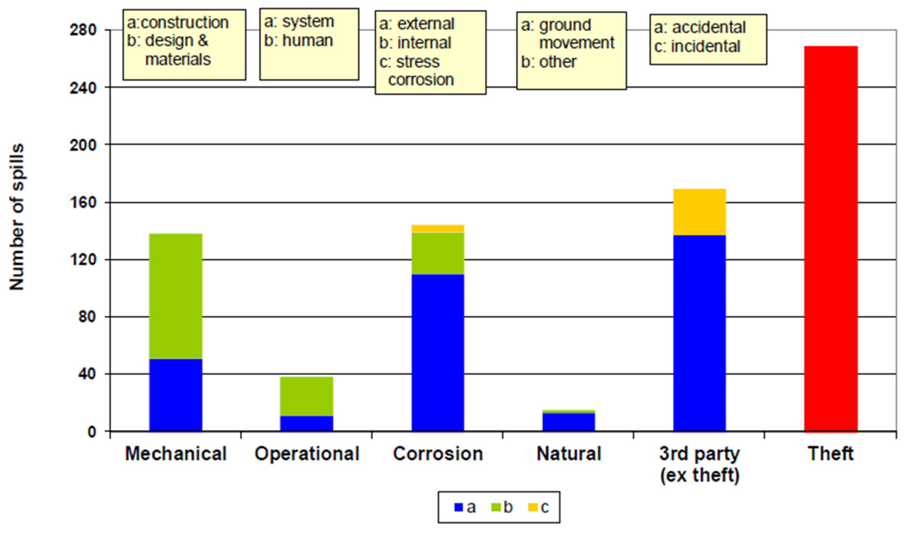
The CONCAWE database has classified oil pipeline failures into five categories [20]: mechanical, corrosion, operational, third-party, and natural hazards. Figure 1 illustrates the contribution of these failures based on data reports from CONCAWE [21].
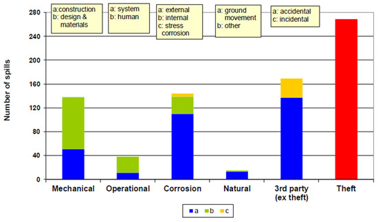
Figure 1.
Number of spills for different failure categories in oil pipelines.
Mechanical failure is caused by design flaws, material faults (e.g., inappropriate or low-quality materials, and incorrect material specification), or construction problems (e.g., poor workmanship, inadequate support, and faulty weld) [22]. These defects can be deformations in the pipe wall in the form of dents and gouges [23]. Dents are radial deformations, whereas gouges are deformations along the pipe surface. This failure type can cause immediate or delayed failure, depending on its severity.
Corrosion is a slow process that results in the loss of metal in the wall, resulting in pipeline failure [24]. Corrosion is the second most common cause of pipeline collapse, according to the U.S. department of transportation. It is divided into internal and external corrosion, as well as stress cracking corrosion. Internal corrosion affects the inner surface of a pipeline and is usually caused by the material being conveyed. It is influenced by two key factors, namely product corrodibility and corrosion intervention. On the contrary, external corrosion occurs as a result of subsurface or atmospheric factors in buried and above-ground pipelines, respectively [25]. Due to its intricate mechanism, subsurface corrosion is more destructive than atmospheric corrosion. Cathodic protection and pipeline coating can help to delay its occurrence [26]. Due to the combined effects of corrosion and tensile stress, material cracking occurs as a result of stress crack corrosion [27].
Operational failure results from operator errors, operational upsets, and failures or inadequacies in safeguarding systems [28]. This failure type is uncommon, despite having disastrous repercussions. In addition to pressure monitoring, the deployment of safety devices, supervisory control and data acquisition communications, and other methods may help to prevent operational failures [29].
Third-party failure is caused by events unrelated to the pipeline [30]. Intentional or accidental third-party operations are the most common failure source in oil pipelines, despite being the least studied factor in pipeline hazard assessment [31]. Cover depth, coating, and public education are among the factors that influence third-party damage.
Natural hazards such as volcanic activity, lightning strikes, earthquakes, land displacement, and flooding are uncommon [32]. To avoid this type of failure, geotechnical and hydrotechnical investigations are conducted before pipeline installation.
3. Materials and Methods
3.1. Multilayer Perceptron Neural Network
The fundamental functions of ANN comprise modeling nonlinear correlations and complex interactions between inputs and outcomes as well as data clustering and classification based on historical data [33,34]. The ANN approach simulates human brain learning and recall of patterns. Neurons (i.e., processing elements), connection pattern, environment, activation state vector, activation rule, signal function, activity aggregation rule, and learning rule are the eight main components of neural networks [35]. The neurons are connected through transfer functions (weights) in three major layers; input, hidden, and output [36]. The inputs are fed into the input layer and they are concurrently sent to the hidden layer(s). The outputs of hidden layers are fed into the output layer, which reports the network’s output [37]. The layers are linked via weights and biases, which impact the predictive capability of the model [38,39,40,41,42]. The weights and biases are modified repeatedly until the appropriate tolerance limit is reached [43].
A multilayer perceptron (MLP) neural network that is trained using a back-propagation learning algorithm is the most commonly used feed-forward neural network. Figure 2 shows the schematic of a back-propagation neural network. The convergence of this network is slow, but it is frequently reliable and accurate [44]. Feed-forward computation, back-propagation to the output and hidden layers, and weight update are the four fundamental steps of a back-propagation algorithm [45]. These steps are repeated until the error is reduced to a satisfactory level.

Figure 2.
Structure of back-propagation neural network.
3.2. Radial Basis Function Neural Network
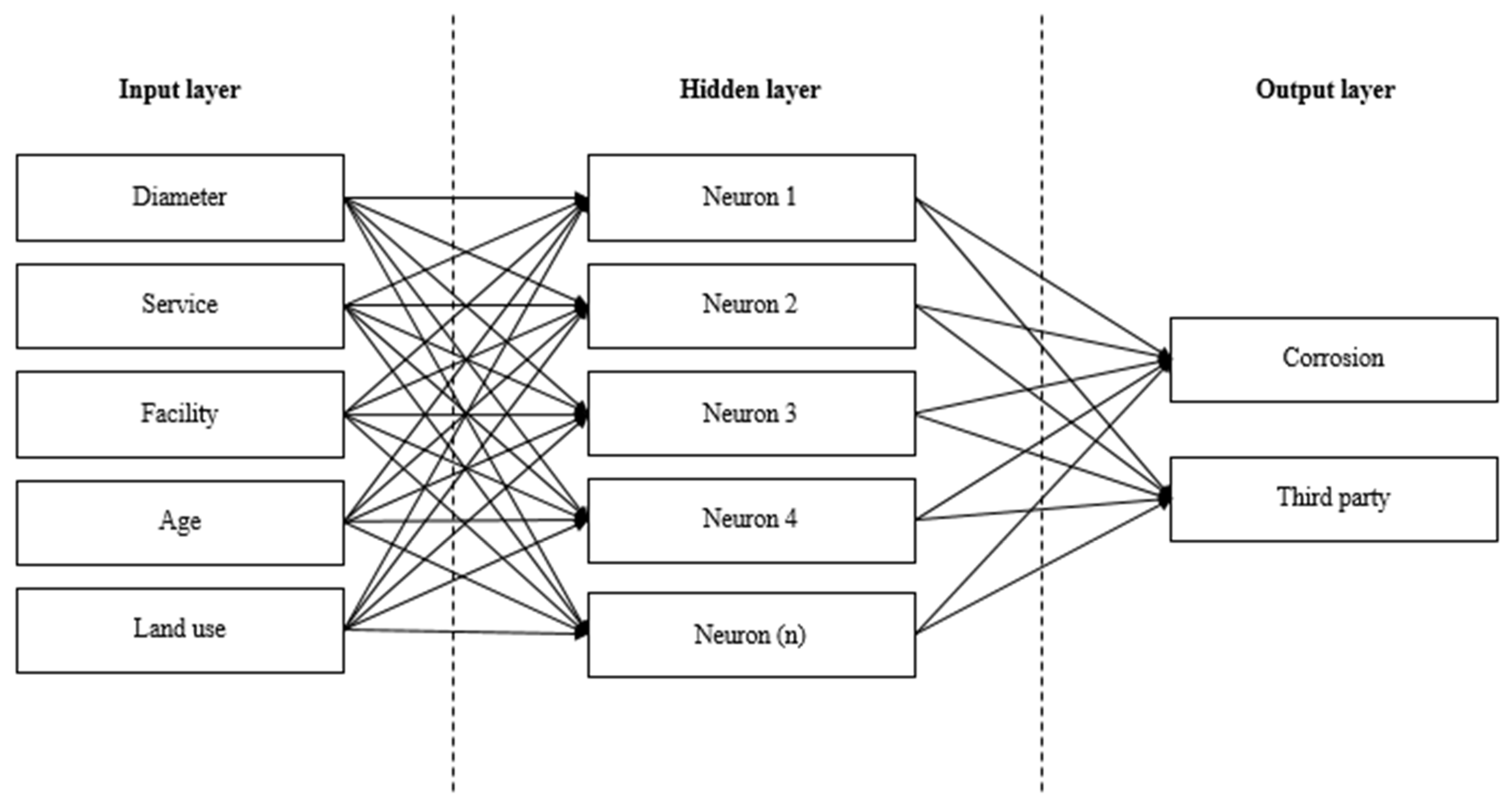
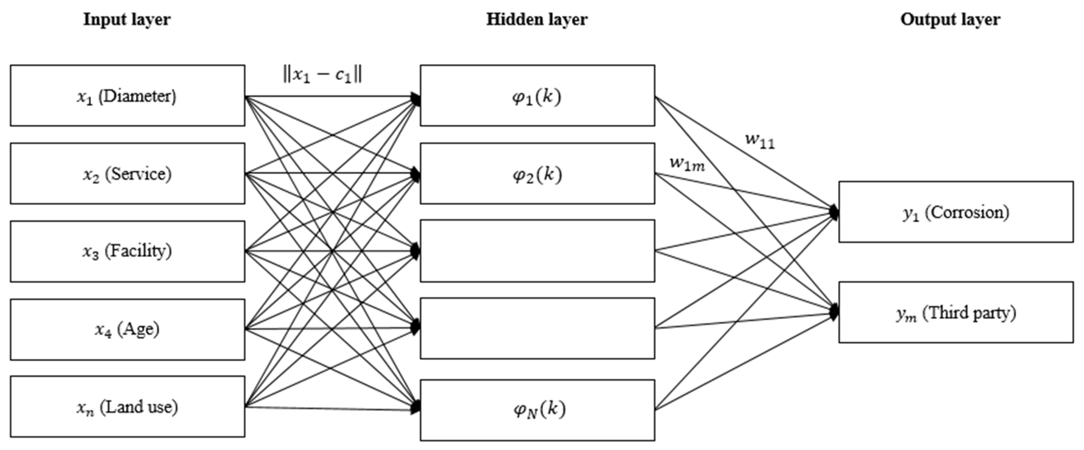
The RBF network was proposed by Moody and Darken in 1980. It has gained prominence in a variety of applications, including time-series prediction, curve fitting, and classification problems. The major strengths of this network are that the local minima can be avoided, the learning process may be substantially accelerated, and any continuous function can be approximated with arbitrary precision [46]. It has the same structure as a feed-forward network that comprises input, hidden, and output layers, as shown in Figure 3. The only distinction is that the input and hidden layers have no connection weights. The output of hidden nodes is calculated using a set of radial basis functions. The input nodes transfer the input values to each of the hidden nodes. Based on the radial basis function, each hidden node generates an activation. Finally, each output node calculates a weighted linear combination of the hidden nodes’ activations, as per Equation (1) [47]. More references about the algorithms for RBF neural network can be found in [48].
where represents the value of an input, is the number of input nodes, refers to the center of the node in the hidden layer, , is the number of hidden nodes, represents the non-linear transfer function of the node, represents the Euclidean distance between and , is the weight value between the output node and node, and refers to the number of output nodes.
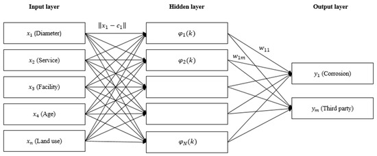
Figure 3.
Structure of radial basis function network.
3.3. Multinomial Regression
Multinomial logistic regression is used to predict categorical dependent variables by employing binomial probability theory. When the dependent variable is dichotomous rather than continuous, binomial logistic regression is used, whereas multinomial logistic regression is utilized when the dependent variable is categorical. Equations (2) and (3) are used to express logistic regression [49,50].
where is the logit formula, is the dependent variable, is the intercept, are the coefficients, are the independent variables, and is the number of explanatory factors.
The following are the limitations of logistic regression [51]: (1) linear relationship between the response and the independent variables, (2) consideration of dichotomous response, (3) presence of mutually exclusive categories, (4) requirement of large sample sizes, (5) non-applicability of using independent variables that are interval-valued, and (6) ineffectiveness of using independent variables that follow the normal or linear distribution.
An MNL model is a logistic regression extension, which sets one of the dependent variables as a reference category. The membership probability of the other dependent categories is then compared to that of the reference category. equations are required to illustrate a relationship between the response and the explanatory factors in a dependent variable with categories. When a dependent variable has more than two categories, the outcome probability is determined using Equation (4). Furthermore, the reference category probability is computed using Equation (5) [49].
4. Data Collection
Failure records provided by CONCAWE in 2019 are used to develop the failure prediction models [21]. The data included 49 years of spillage data dating back to 1971, as well as 36,000 km of pipelines transporting 620 million m3 of crude oil and petroleum products per year across Europe. A total of 73 agencies and organizations operating around 35,691 km of oil pipelines provide annual data for the CONCAWE study. In 2019, the total transported amount of crude oil and processed products was roughly 619 mm3 while the overall traffic volume was anticipated to be 119 × 109 m3 per km.
Six spillage incidents were recorded in 2019, equivalent to 0.18 spillages per 1000 km of line. This value is much lower than the annual average of 0.44, which has been declining from a value of 1.1 in the mid-1970s. Two out of the six recorded incidents were caused by mechanical failures, one by operational issues, three by corrosion, and none by natural hazards and intentional or accidental third-party activity. There have been no recorded injuries, deaths, or fires as a result of these spills. The gross spillage volume was 961 m3 (28.3 m3 per 1000 km of pipeline), compared to the long-term average of 62 m3 per 1000 km. It was reported that 93% of the spillage volume was collected or disposed of securely.
CONCAWE database includes 586 records for the five different failure causes (i.e., mechanical, operational, corrosion, natural hazards, and third-party). It is noted that a total of 232 event records are lacking data for certain factors. As a consequence, these incidents are removed from the database, maintaining 354 incidents with complete data. The utilized dataset comprises 253 accidents owing to corrosion and third-party activities. Accidents caused by mechanical, operational, and natural hazards are not recorded in the dataset due to their low probabilities of occurrences. Table 1 depicts a sample of the database used for building the model. Each spilled incidence represents a unique instance and is distinguished by five distinct characteristics in addition to the primary cause/type of failure. Pipeline diameter, service type, facility type, age, and land use are all considered explanatory variables. The model excludes the gross and net loss spillage volume, leak detection method, and facility part variables. This can be attributed to the impossibility of determining these variables before a failure occurs, yet the established model is designed to anticipate the failure cause before its occurrence.

Table 1.
CONCAWE database sample for the developed models.
5. Model Development
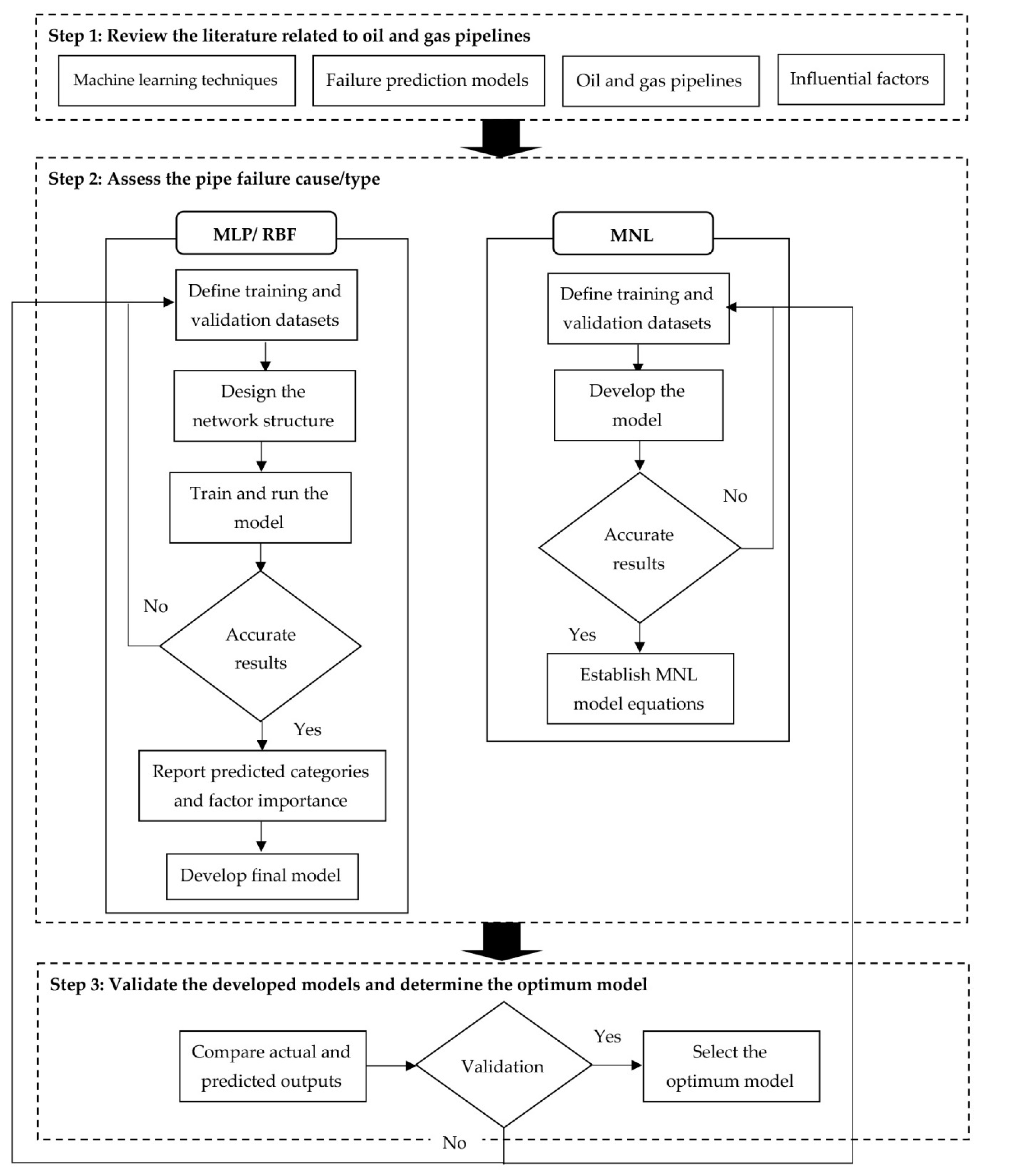
The failure prediction model development is illustrated in Figure 4. The data extracted from the CONCAWE study is utilized to estimate the condition of oil pipelines. MLP and RBF neural networks, as well as MNL regression models, are developed to forecast different failure types using SPSS 28 statistical software [52]. To build the models, the dataset is randomly divided into 70% and 30% for training and validation, respectively. As depicted in Table 2, the input factors (i.e., diameter, service, facility, age, and land use) are the key predictors of the developed models, whereas the main output is the failure type. The three qualitative factors (service, facility, and land use) have been incorporated into the model after being converted into numeric values. Furthermore, the other two quantitative parameters (age and diameter) have varying units of measure. As a result, the values of the input and output factors must be normalized. As a consequence, the models are designed to forecast the failure type based on various combinations of input categories.
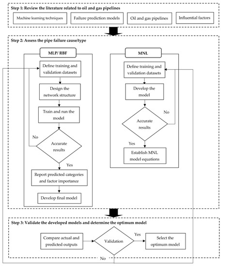
Figure 4.
Research methodology.
Table 2.
Data gathered for the construction of a model.
5.1. MLP and RBF Models
The network architecture is influenced by the selected input and output variables. Each variable is represented by a single artificial neuron. As a result, the network architecture has five neurons in the input layer and two in the output layer. The appropriate number of hidden neurons is determined after conducting several iterations. For MLP, the activation functions in the hidden and output layers are hyperbolic tangent and softmax, respectively. Additionally, the stopping rule used is one consecutive step with no error decrease. By adjusting connection weights, a scaled conjugate gradient optimization algorithm is employed to minimize the objective function (error). Meanwhile, for RBF, softmax and identity are the activation functions in the hidden and output layers, respectively.
5.2. MNL Model
The likelihood of each output category (i.e., failure type) is computed using multinomial regression, which helps to identify the most likely and critical failure sources. The highest probability is assigned as the anticipated value. Each category is associated with a baseline in the logit model, and third-party failure is utilized as the baseline in this research. The model performance is measured using the maximum-likelihood estimate, which indicates the similarity between the observed and modeled parameter values. It is commonly equal to 2 log-likelihood (2 LL) [50,53].
Several pseudo-R squares are utilized to evaluate the goodness of fit for the MNL models, as per Equations (6)–(8) [54,55,56]. These metrics resemble R-square such that they range from 0 to 1, with higher values indicating better model fit and vice versa.
where and denote models without and with predictors, respectively. Furthermore, denotes the estimated likelihood, and denotes the number of data points.
The initial likelihood for the reduced model, which omits the effect of the investigated variable, is estimated to determine each predictor’s importance. This probability is compared against the reported results when considering all predictors (full model). The chi-square for each predictor is then determined by subtracting the full model value from the reduced model value. The predictor is deemed significant when it is associated with high chi-square and low significance values.
6. Model Validation
The purpose of this step is to validate and test the prediction effectiveness of the developed models. Equations (9) and (10) are used to calculate the average invalidity percentage (AIP) and average validity percentage (AVP). The model is sound if the AIP value is closer to 0, while the prediction capability of the model is not acceptable if the AIP value is closer to 100 [57].
where refers to the number of records and and refer to the estimated and actual values, respectively.
The second approach for computing the AIP is adopted by dividing the number of inaccurate predictions () by the overall number of records (), as per Equation (11).
7. Results and Discussion
MLP and RBF neural networks, as well as MNL regression models, are developed to forecast corrosion and third-party failures. For MLP and RBF models, the optimum number of hidden neurons is determined to be three and ten neurons, respectively. As depicted in Table 3, the findings of the importance factor analysis for MLP reveal that the order of importance of the predictors is listed in the following order: facility, service, land use, age, and diameter. On the other hand, for the RBF model, the predictors are arranged in the following order of importance: service, facility, land use, age, and diameter.
Table 3.
Assessment of the importance of inputs in the neural network models.
The receiver operating characteristic (ROC) curve is a diagnostic method for evaluating classification problems. To evaluate classifier performance in differentiating positive and negative data, it plots the true positive rate versus the false positive rate. A bigger area under the ROC curve suggests a better likelihood of classification as a positive rather than a negative value. Table 4 demonstrates that the area under the ROC curve for each dependent variable category in the MLP model is often greater than 0.7, indicating good prediction accuracy. However, for the RBF model, the area under the ROC curve = 0.8, indicating very good prediction accuracy.
Table 4.
Area under the curve for the neural network models.
As shown in Table 5, the likelihood function value for the MNL model without independent variables is 305.642, whereas the value with all independent variables is 293.395. Due to the inclusion of independent variables, a decrease in this value reflects improved model prediction. The chi-square (12.246) has a significance of 0.032, indicating a statistically significant association between the explanatory and response variables [53]. Moreover, the pseudo–R square findings are summarized in Table 6.
Table 5.
MNL model fitting information.
Table 6.
Pseudo R-square values for the MNL model.
Table 7 summarizes the likelihood ratio test analysis findings. It reveals that the most influential variable is facility type because it is associated with the highest chi-square (5.891) and lowest significance (0.015) values.
Table 7.
Likelihood ratio test for the MNL model.
As previously explained, the MNL regression model is based on calculating the likelihood of each failure type that is based on computing the logit of each output. In this context, the variable coefficients of the dependent variables are depicted in Table 8. The logit for corrosion and third-party failures is calculated using Equations (12) and (13).
Table 8.
Parameter estimations for the MNL model.
Finally, the likelihood of each failure source is computed using Equations (14) and (15).
Table 9 summarizes the results of the training and validation phases for the MLP, RBF, and MNL models. For the first approach, the AVP values for the MLP, RBF, and MNL models are 0.84, 0.86, and 0.80, respectively, in the training phase. Meanwhile, for the validation phase, the AVP values are 0.85, 0.83, and 0.82 for the MLP, RBF, and MNL models, respectively. For the training and validation phases, the MLP, RBF, and MNL models predict failure causes with AVP values of 0.84, 0.85, and 0.81, respectively. The average validity percentage in all models is above 0.80, indicating very good classification accuracy. The findings confirm the robustness of the developed RBF model and its ability to forecast pipeline failure based on a set of input variables. However, the prediction accuracy of models could have been compromised due to the non-availability of some important factors (e.g., thickness, operating pressure, and yield strength) that contribute to oil and gas pipeline failure. Furthermore, due to confidentiality concerns, access to a significant number of failure records in the oil and gas industry is often difficult.
Table 9.
Findings of the training and validation phases for the classification models.
For the training phase, the findings of the second approach indicate that the AVP values are 0.74, 0.77, and 0.70 for the MLP, RBF, and MNL models, respectively. Meanwhile, for the validation phase, the AVP values are 0.79, 0.70, and 0.72 for the MLP, RBF, and MNL models, respectively. It should also be noted that the AVP values acquired using the second approach are lower than those reported using the first approach. The reason is that, in the second approach, the event is utterly incorrect if the anticipated failure type differs from the actual one. On the contrary, the first approach adopts estimating the deviation between the actual and modeled failure types. Despite this, the second approach produces satisfactory AVP results for the models.
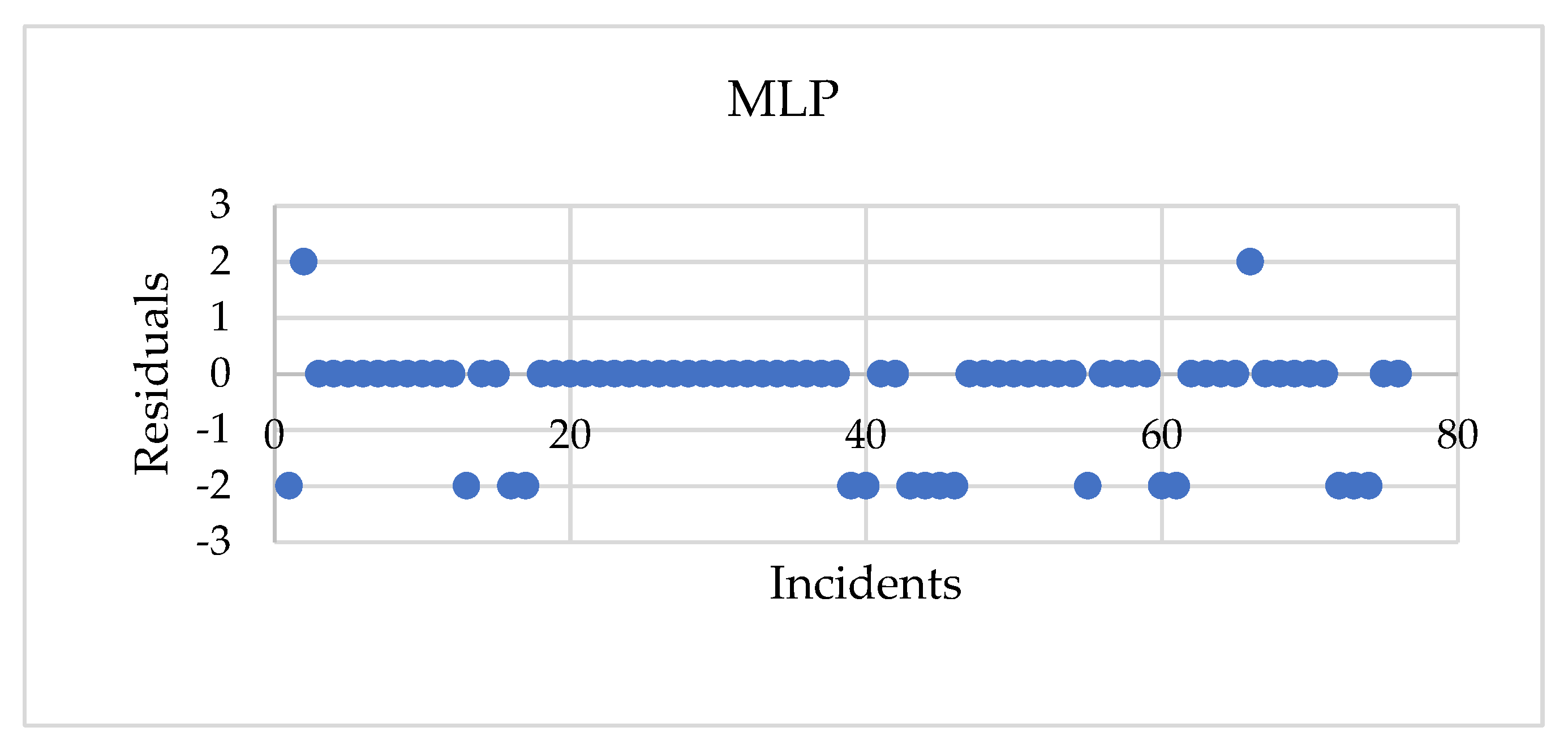
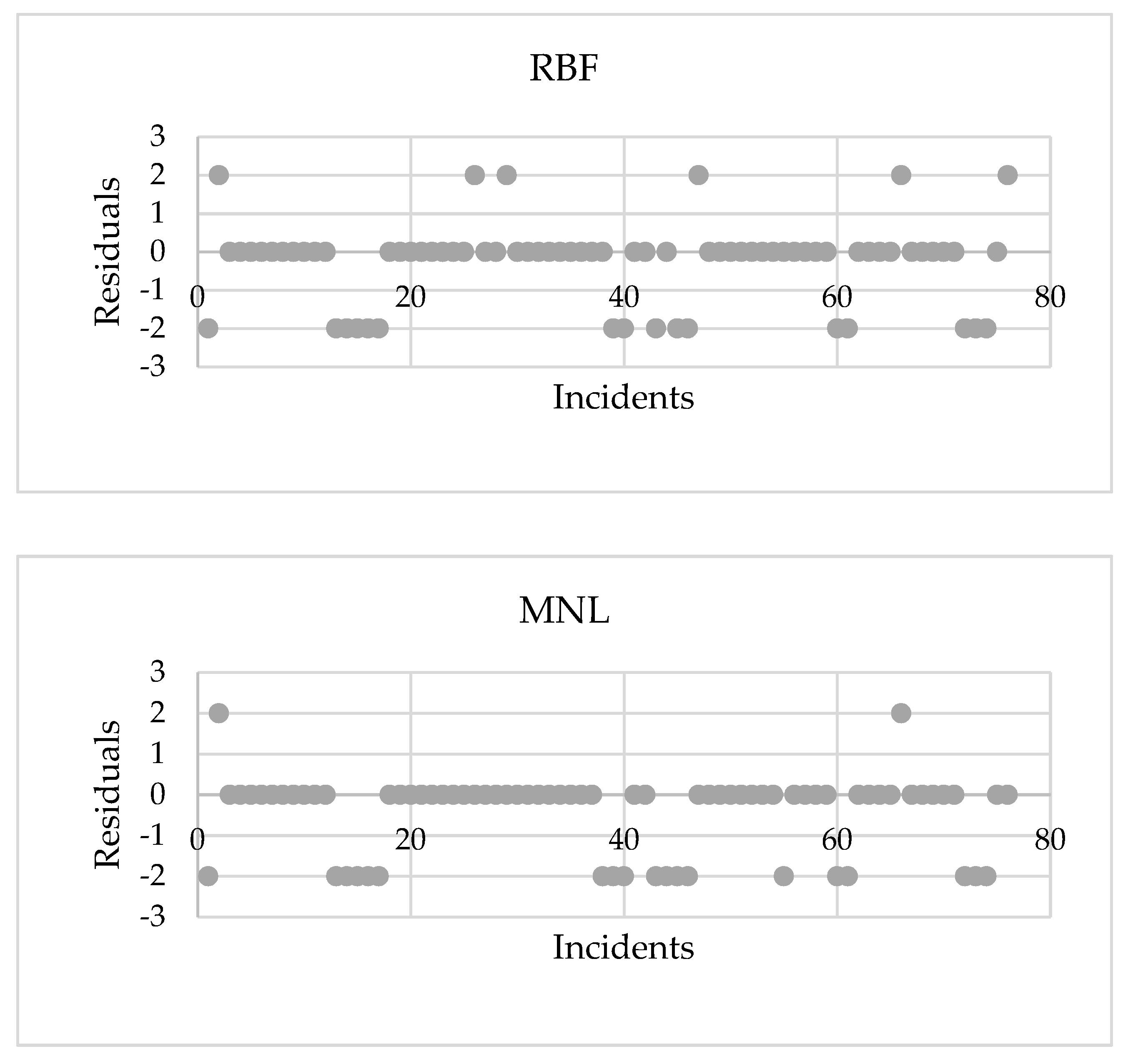
Figure 5 illustrates the residual plots for the actual and modeled failure types using classification models. The mean of errors is −0.37, −0.26, and −0.45 for the MLP, RBF, and MNL models, respectively. Meanwhile, the standard deviation of the measured errors ranges between 0.91 and 1.05 for the classification models. This figure shows that the predicted values of the three models are within acceptable bounds and are distributed around the actual values. The MLP and RBF models outperform the MNL regression model in terms of accuracy because they take into account the nonlinear relationship between the dependent and independent variables, as well as the correlation between the parameters that determine the pipeline failure cause.
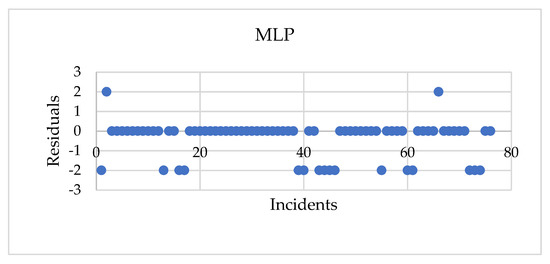
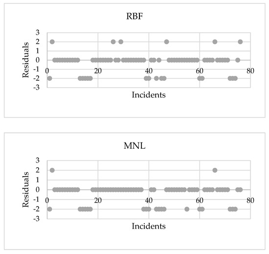
Figure 5.
Residual plots for MLP, RBF, and MNL models.
The outcomes of the established models are compared to the results reported in the literature. Zakikhani et al. [17] presented an ANN model that was associated with an AVP of 0.728 for forecasting corrosion and third-party failures in oil pipelines based on physical, environmental, and operational factors. In this research, the developed MLP, RBF, and MNL models are associated with AVP values of 0.84, 0.85, and 0.81, respectively. This implies that the proposed MLP, RBF, and MNL models enhanced the AVP value reported in the literature by 15.4%, 16.8%, and 11.3%, respectively. Therefore, the proposed RBF model outperforms previously published models, emphasizing its robustness and accuracy capabilities.
8. Conclusions
This research study developed three models for predicting corrosion and third-party failures in oil pipelines, taking into account several predictors such as age, diameter, facility, service, and land use. Findings showed that these failure categories accounted for more than 70% of total oil pipeline accidents. The models were developed using multilayer perceptron (MLP) neural network, radial basis function (RBF) neural network, and multinomial logistic (MNL) regression. The importance factor analysis for MLP revealed that the order of importance of the predictors was as follows: facility, service, land use, age, and diameter. On the other hand, for the RBF model, the predictors were arranged in the following order of importance: service, facility, land use, age, and diameter. For MNL, the likelihood ratio test analysis revealed that the most influential variable was facility type because it was associated with the highest chi-square and lowest significance values. Moreover, the model calculated the likelihood of each failure source, assisting decision makers in determining the most likely and critical failure sources. For MLP and RBF neural networks, the area under the receiver operating characteristic (ROC) curve for each dependent variable category was about 0.7 and 0.8, respectively, indicating good prediction accuracy. The MLP, RBF, and MNL models predicted failure causes with AVP values of 0.84, 0.85, and 0.81, respectively. The developed models were tested for robustness against other previous models based on AVP value. It was found that the proposed MLP, RBF, and MNL models enhanced the AVP value reported in the literature by 15.4%, 16.8%, and 11.3%, respectively. Therefore, the proposed RBF model outperformed previously published models, emphasizing its robustness and accuracy capabilities. This can be attributed to the fact that the RBF model accounted for the nonlinear relationship between the dependent and independent variables, as well as the correlation between the parameters that determined the pipeline failure cause. The established models provide decision makers with a clear picture of the failure sources that endanger a pipeline, allowing them to mitigate risks and ensure pipe safety. These models can assist oil pipeline operators and decision makers in planning pipeline safety by forecasting how pipelines will break based on specific physical, operational, and environmental features. It is recommended in the future to examine the performance of the developed models for predicting other failure types (e.g., mechanical, operational, and natural hazards) in oil and gas pipelines.
Author Contributions
Conceptualization, N.E. and E.M.A.; methodology, N.E. and E.M.A.; formal analysis N.E., E.M.A., A.A.-S. and G.A.; data curation, N.E., E.M.A., A.A.-S. and G.A.; Investigation, N.E., E.M.A., A.A.-S. and G.A.; Resources, N.E., E.M.A., A.A.-S. and G.A.; writing—original draft preparation, N.E., E.M.A., A.A.-S. and G.A.; and writing—review and editing, N.E., E.M.A., A.A.-S. and G.A. All authors have read and agreed to the published version of the manuscript.
Funding
This research received no external funding.
Institutional Review Board Statement
Not applicable.
Informed Consent Statement
Informed consent was obtained from all subjects involved in the study.
Data Availability Statement
Some or all data, models, or code that support the findings of this study are available from the corresponding author upon reasonable request.
Conflicts of Interest
The authors declare no conflict of interest.
References
- Zhang, P.; Qin, G.; Wang, Y. Risk assessment system for oil and gas pipelines laid in one ditch based on quantitative risk analysis. Energies 2019, 12, 981. [Google Scholar] [CrossRef] [Green Version]
- Abdoul Nasser, A.H.; Ndalila, P.D.; Mawugbe, E.A.; Emmanuel Kouame, M.; Arthur Paterne, M.; Li, Y. Mitigation of risks associated with gas pipeline failure by using quantitative risk management approach; A descriptive study on gas industry. J. Mar. Sci. Eng. 2021, 9, 1098. [Google Scholar] [CrossRef]
- Kennedy, J.L. Oil and Gas Pipeline Fundamentals, 2nd ed.; PennWell: Tulsa, OK, USA, 1993. [Google Scholar]
- WorldAtlas. Top 20 Countries By Length of Pipeline. Available online: https://www.worldatlas.com/articles/top-20-countries-by-length-of-pipeline.html (accessed on 25 October 2021).
- Statista. Number of Oil Pipelines Globally by Status 2020. Available online: https://www.statista.com/statistics/1131423/oil-pipelines-by-status-worldwide/ (accessed on 25 October 2021).
- Energy Minute. Visualizing Future Pipeline Projects Around the World. Available online: https://energyminute.ca/single/infographics/1120/pipelines-in-2021 (accessed on 25 October 2021).
- Dey, P.; Ogunlana, S.; Naksuksakul, S. Risk-based maintenance model for offshore oil and gas pipelines: A case study. J. Qual. Maint. Eng. 2004, 10, 169–183. [Google Scholar] [CrossRef]
- Davis, M.; Dubois, J.; Gambardella, F.; Uhlig, F. Performance of European Cross-Country Oil Pipelines: Statistical Summary of Reported Spillages in 2008 and Since 1971; CONCAWE Oil Pipelines Management Group, Special Task Force: Brussels, Belgium, 2010. [Google Scholar]
- Shaik, N.B.; Pedapati, S.R.; Taqvi, S.A.A.; Othman, A.R.; Dzubir, F.A.A. A feed-forward back propagation neural network approach to predict the life condition of crude oil pipeline. Processes 2020, 8, 661. [Google Scholar] [CrossRef]
- Kabir, G.; Sadiq, R.; Tesfamariam, S. A fuzzy Bayesian belief network for safety assessment of oil and gas pipelines. Struct. Infrastruct. Eng. 2016, 12, 874–889. [Google Scholar] [CrossRef]
- Li, J.; Zhang, H.; Han, Y.; Wang, B. Study on failure of third party damage for urban gas pipeline based on fuzzy comprehensive evaluation. PLoS ONE 2016, 11, e0166472. [Google Scholar] [CrossRef]
- Dundulis, G.; Žutautaitė, I.; Janulionis, R.; Ušpuras, E.; Rimkevičius, S.; Eid, M. Integrated failure probability estimation based on structural integrity analysis and failure data: Natural gas pipeline case. Reliab. Eng. Syst. Saf. 2016, 156, 195–202. [Google Scholar] [CrossRef]
- Zhou, Q.; Wu, W.; Liu, D.; Li, K.; Qiao, Q. Estimation of corrosion failure likelihood of oil and gas pipeline based on fuzzy logic approach. Eng. Fail. Anal. 2016, 70, 48–55. [Google Scholar] [CrossRef]
- Abdrabou, B. Failure Prediction Model for Oil Pipelines. Master’s Thesis, Concordia University, Montreal, QC, Canada, 2012. [Google Scholar]
- El-Abbasy, M.S.; Senouci, A.; Zayed, T.; Mirahadi, F.; Parvizsedghy, L. Artificial neural network models for predicting condition of offshore oil and gas pipelines. Autom. Constr. 2014, 45, 50–65. [Google Scholar] [CrossRef]
- Senouci, A.; Elabbasy, M.; Elwakil, E.; Abdrabou, B.; Zayed, T. A model for predicting failure of oil pipelines. Struct. Infrastruct. Eng. 2014, 10, 375–387. [Google Scholar] [CrossRef]
- Zakikhani, K.; Zayed, T.; Abdrabou, B.; Senouci, A. Modeling failure of oil pipelines. J. Perform. Constr. Facil. 2020, 34, 04019088. [Google Scholar] [CrossRef]
- Zakikhani, K.; Nasiri, F.; Zayed, T. A failure prediction model for corrosion in gas transmission pipelines. Proc. Inst. Mech. Eng. O J. Risk Reliab. 2021, 235, 374–390. [Google Scholar] [CrossRef]
- Zakikhani, K.; Nasiri, F.; Zayed, T. A review of failure prediction models for oil and gas pipelines. J. Pipeline Syst. Eng. Pract. 2020, 11, 03119001. [Google Scholar] [CrossRef]
- Lyons, D. Western European Cross-Country Oil Pipelines 30-Year Performance Statistics; Concawe: Brussels, Belgium, 2002. [Google Scholar]
- Larive, J.F. Performance of European Cross-Country Oil Pipelines. Statistical Summary of Reported Spillages in 2019 and Since 1971. Available online: https://www.concawe.eu/wp-content/uploads/Rpt_21-4.pdf (accessed on 25 October 2021).
- Orasheva, J. The Effect of Corrosion Defects on the Failure of Oil and Gas TRANSMISSION pipelines: A Finite Element Modeling Study. Master’s Thesis, University of North Florida, Jacksonville, FL, USA, 2017. [Google Scholar]
- Murugathasan, P.; Muntakim, A.H.; Dhar, A.S. Nonlinear finite element analysis of dented pipes under internal pressure and axial loads. AIP Conf. Proc. 2021, 2324, 030025. [Google Scholar]
- Popoola, L.T.; Grema, A.S.; Latinwo, G.K.; Gutti, B.; Balogun, A.S. Corrosion problems during oil and gas production and its mitigation. Int. J. Ind. Chem. 2013, 4, 35. [Google Scholar] [CrossRef] [Green Version]
- Syromyatnikova, A.; Bolshakov, A.; Ivanov, A.; Alexeev, A.; Bolshev, K.; Andreev, Y. The corrosion damage mechanisms of the gas pipelines in the Republic of Sakha (Yakutia). Procedia Struct. Integr. 2019, 20, 259–264. [Google Scholar] [CrossRef]
- Ossai, C.I. Advances in asset management techniques: An overview of corrosion mechanisms and mitigation strategies for oil and gas pipelines. Int. Sch. Res. Notices 2012, 2012, 570143. [Google Scholar] [CrossRef] [Green Version]
- Khalifeh, A. Stress corrosion cracking behavior of materials. Eng. Fail. Anal. 2020. [Google Scholar] [CrossRef]
- Bersani, C.; Citro, L.; Gagliardi, R.; Sacile, R.; Tomasoni, A. Accident occurrence evaluation in the pipeline transport of dangerous goods. Chem. Eng. Trans. 2010, 19, 249–254. [Google Scholar]
- Aba, E.N.; Olugboji, O.A.; Nasir, A.; Olutoye, M.A.; Adedipe, O. Petroleum pipeline monitoring using an internet of things (IoT) platform. SN Appl. Sci. 2021, 3, 1–12. [Google Scholar] [CrossRef]
- Santarelli, J.S. Risk Analysis of Natural Gas Distribution Pipelines with Respect to Third Party Damage. Master’s Thesis, Western University, London, ON, Canada, 2019. [Google Scholar]
- Muhlbauer, W.K. Pipeline Risk Management Manual: Ideas, Techniques, and Resources; Gulf Professional Publishing: Amsterdam, The Netherlands, 2004. [Google Scholar]
- Girgin, S.; Krausmann, E. Analysis of Pipeline Accidents Induced by Natural Hazards; European Union: Brussels, Belgium, 2014. [Google Scholar]
- Abiodun, O.I.; Jantan, A.; Omolara, A.E.; Dada, K.V.; Mohamed, N.A.; Arshad, H. State-of-the-art in artificial neural network applications: A survey. Heliyon 2018, 4, e00938. [Google Scholar] [CrossRef] [PubMed] [Green Version]
- Malekian, A.; Chitsaz, N. Concepts, procedures, and applications of artificial neural network models in streamflow forecasting. In Advances in Streamflow Forecasting; Elsevier: Amsterdam, The Netherlands, 2021; pp. 115–147. [Google Scholar]
- Rao, S.; Kumari, V.; Rao, P. Image compression using neural network for biomedical applications. In Soft Computing for Problem Solving; Springer: Singapore, 2019; pp. 107–119. [Google Scholar]
- Uzair, M.; Jamil, N. Effects of Hidden Layers on the Efficiency of Neural Networks. In Proceedings of the 2020 IEEE 23rd International Multitopic Conference (INMIC), Bahawalpur, Pakistan, 5–7 November 2020. [Google Scholar]
- Alaloul, W.S.; Qureshi, A.H. Data processing using artificial neural network. In Dynamic Data Assimilation-Beating the Uncertainties; IntechOpen: London, UK, 2020. [Google Scholar]
- Elkatatny, S.; Mahmoud, M.; Tariq, Z.; Abdulraheem, A. New insights into the prediction of heterogeneous carbonate reservoir permeability from well logs using artificial intelligence network. Neural. Comput. Appl. 2018, 30, 2673–2683. [Google Scholar] [CrossRef]
- Elkatatny, S.; Tariq, Z.; Mahmoud, M.; Abdulraheem, A. New insights into porosity determination using artificial intelligence techniques for carbonate reservoirs. Petroleum 2018, 4, 408–418. [Google Scholar] [CrossRef]
- Tariq, Z.; Mahmoud, M.; Abdulraheem, A. Real-time prognosis of flowing bottom-hole pressure in a vertical well for a multiphase flow using computational intelligence techniques. J. Pet. Explor. Prod. Technol. 2020, 10, 1411–1428. [Google Scholar] [CrossRef] [Green Version]
- Tariq, Z.; Mahmoud, M. New correlation for the gas deviation factor for high-temperature and high-pressure gas reservoirs using neural networks. Energy Fuels 2019, 33, 2426–2436. [Google Scholar] [CrossRef]
- Desouky, M.; Tariq, Z.; Aljawad, M.S.; Alhoori, H.; Mahmoud, M.; AlShehri, D. Data-driven acid fracture conductivity correlations honoring different mineralogy and etching patterns. ACS Omega 2020, 5, 16919–16931. [Google Scholar] [CrossRef]
- Rezakazemi, M.; Razavi, S.; Mohammadi, T.; Nazari, A. Simulation and determination of optimum conditions of pervaporative dehydration of isopropanol process using synthesized PVA–APTEOS/TEOS nanocomposite membranes by means of expert systems. J. Membr. Sci. 2011, 379, 224–232. [Google Scholar] [CrossRef]
- Ecer, F.; Ardabili, S.; Band, S.S.; Mosavi, A. Training multilayer perceptron with genetic algorithms and particle swarm optimization for modeling stock price index prediction. Entropy 2020, 22, 1239. [Google Scholar] [CrossRef]
- Han, J.; Kamber, M.; Pei, J. Classification: Advanced Methods. In The Morgan Kaufmann Series in Data Management Systems, Data Mining, 3rd ed.; Morgan Kaufmann Publishers: Waltham, MA, USA, 2012; pp. 393–442. [Google Scholar]
- Sun, Z.; Deng, Z.; Zhang, Z. Intelligent Control Theory and Technology, 2nd ed.; Tsinghua University Press: Beijing, China, 2016. [Google Scholar]
- Dash, R.; Dash, P.K. A Comparative Study of Radial Basis Function Network with Different Basis Functions for Stock Trend Prediction. In Proceedings of the 2015 IEEE Power, Communication and Information Technology Conference (PCITC), Bhubaneswar, India, 15–17 October 2015. [Google Scholar]
- Stastny, J.; Skorpil, V. Analysis of algorithms for radial basis function neural network. In Personal Wireless Communications; Springer: Boston, MA, USA, 2007; pp. 54–62. [Google Scholar]
- Agresti, A. An Introduction to Categorical Data Analysis; Wiley: Hoboken, NJ, USA, 2007. [Google Scholar]
- Withers, S.D. Data analysis, categorical. In International Encyclopedia of Human Geography, 2nd ed.; Elsevier: Amsterdam, The Netherlands, 2009; pp. 159–165. [Google Scholar]
- Burns, B.; Burns, R. Business Research Methods and Statistics Using SPSS; SAGE: London, UK, 2008. [Google Scholar]
- IBM Corp. IBM SPSS Statistics for Windows; IBM Corp: Armonk, NY, USA, 2017. [Google Scholar]
- Menard, S. Applied Logistic Regression Analysis; SAGE: Thousand Oaks, CA, USA, 2002. [Google Scholar]
- McFadden, D. Conditional logit analysis of qualitative choice behavior. In Frontiers in Econometrics; Zarembka, P., Ed.; Academic Press: New York, USA, 1974; pp. 105–142. [Google Scholar]
- Cox, D.R.; Snell, E.J. Analysis of Binary Data; CRC Press: Boca Raton, FL, USA, 1989. [Google Scholar]
- Nagelkerke, N.J. A note on a general definition of the coefficient of determination. Biometrika 1991, 78, 691–692. [Google Scholar] [CrossRef]
- Kaddoura, K. Performance Modeling for Sewer Networks. Ph.D. Thesis, Concordia University, Montreal, QC, Canada, 2018. [Google Scholar]
Publisher’s Note: MDPI stays neutral with regard to jurisdictional claims in published maps and institutional affiliations. |
© 2022 by the authors. Licensee MDPI, Basel, Switzerland. This article is an open access article distributed under the terms and conditions of the Creative Commons Attribution (CC BY) license (https://creativecommons.org/licenses/by/4.0/).