Sensor Fault Detection Combined Data Quality Optimization of Energy System for Energy Saving and Emission Reduction

Abstract

China’s “dual carbon” goals, energy conservation and emission reduction in the energy system, have become increasingly important. The sensor fault of an energy system will cause unstable operation and increase energy consumption. Therefore, this study proposes a new sensor fault detection strategy based on the data driven method for energy saving and emission reduction. However, for data-driven models, data quality has a greater impact on model performance. This study innovatively uses five machine learning methods to optimize the energy system operating data. Five machine learning methods include the moving average (MA), Lowess, Loess, Rlowess and Rloess methods. Fault detection performances of different data driven models optimized by different approaches are compared and analyzed. Besides, data outliers and parameter selection of data optimization methods are discussed. The results indicate that the MA method has the best optimization performance when the smoothness degree is level 2. The optimized data fluctuation range is controlled within the range of ±1. The fault detection accuracy rate of the model optimized based on the MA method is increased from 32.51% to 83.96% when the evaporation temperature sensor fault is a 5 °C deviation. However, the data will deviate from the original data trend when the smoothing parameter is set too large. Therefore, the smoothness of the data should not be too large. The approach proposed in this study is of great significance to the energy saving and emission reduction of the energy system.

1. Introduction

With the development of society, the energy consumption of buildings has been increasing year by year, which has accounted for nearly 40% of the world’s major energy needs [1]. Among them, air conditioning and heating and ventilation systems account for nearly 50% of the total energy consumption of buildings [2,3]. Therefore, the energy saving of the air conditioning system is of great significance to the energy saving and emission reduction of the building [4]. With the launch of China’s “double carbon” policy, building energy saving and emission reduction will become more important [5,6,7]. Sensors are important to the normal operation of the air conditioning system. The faults of the sensor will cause the system to run erratically, deviate from the normal operating mode, and increase the energy consumption [8,9,10]. Therefore, sensor fault detection is very meaningful for building energy saving and emission reduction and has received more and more attention.

Sensor fault detection of the heating, ventilation and air conditioning (HVAC) system can be simply divided into two categories based on historical data [11,12,13] and based on physical knowledge [14,15]. Data-driven methods have become the research focus due to their fast modeling speed and strong generalization ability. Shahnazari et al. [16] proposed a fault detection and isolation strategy of the HVAC system based on recurrent neural networks. Wang et al. [17] established a novel decentralized flat sensor diagnosis network for HVAC system. The results indicate that the proposed method can be effective. Yan et al. [18] developed an unsupervised machine learning based sensor fault detection strategy using cluster analysis for the AHU system. The developed model is capable of detecting single sensor and multiple sensor faults. Besides, the improved sensor fault detection strategy is developed combining density-based clustering with principal component analysis (PCA) method [19]. Montazeri et al. [20] used the RBF, PCA, and KPCA methods for diagnosing nine sensor and actuator faults simultaneously of the AHU system. There is some research on the application of the PCA method in the sensor fault detection for chiller [21,22], AHU [23,24], VRF [25], and other HVAC systems [10,26]. Through the analysis of related research on sensor faults, it can be concluded that the most widely used method for sensor fault detection and diagnosis in the field of air conditioners is principal component analysis. The model established by the principal component analysis method can effectively detect the fault. Therefore, the PCA method is selected to establish the sensor fault detection model for the chiller in this study.

One challenge of data-driven chiller sensor fault detection models is the data quality. The quality of the data determines the performance of the model. Li et al. [27]. used the wavelet transform method to remove the influence of weather condition change. Then, a combined wavelet-PCA model was established for the AHU system. Zhu et al. [28] combined neural network, wavelet, and fractal methods to establish the sensor fault diagnosis model. Compared with the previous model, the fault diagnosis performance can be improved by up to 15% at the same fault level. Besides, the ensemble empirical mode decomposition method is used to optimize the data and the improved PCA based sensor fault detection model is established [29]. Comparing and analyzing related research, the performance of the model after data quality optimization has been improved. In addition, there are other data optimization methods, such as the moving average (MA) data smoothing method [30] and the local regression smoothing approach [31]. However, these data optimization methods have not been used in the field of sensor fault detection. The data optimization effects of these methods have not been studied. The performance of the sensor fault detection model established by the data optimized by these methods is unknown.

According to the above challenge and limitation, this study proposes a new sensor fault detection strategy. First, the data of the fault detection model is optimized by the MA, Lowess, Loess, Rlowess and Rloess methods. Then, the PCA method is used to establish an optimized fault detection model for the chiller. This study compares and analyzes the data optimization performance of the different methods and the fault detection results of different optimized fault detection models. Besides, problems of data outliers and data optimization methods parameter selection are discussed.

2. Methodology

The optimized sensor fault detection strategy proposed in this study mainly includes three parts. The first part is data optimization, including five data smoothing methods, namely moving average, Lowess, Loess, Rlowess, and Rloess methods. Different optimization methods are used individually to optimize the chiller operation data, and the data optimization performance is compared and analyzed. The second part is the fault detection model training. The last part is sensor fault detection. The detailed sensor fault detection strategy optimized by the multiple data smoothing methods is shown in Figure 1.

2.1. Data Optimization Methods

2.1.1. The Moving Average Data Smoothing Method

The moving average (MA) filter is a common method for smoothing noisy data. This method smooths data by replacing data points with the average of adjacent data points within a selected window width. This process can also be equivalent to a low-pass filter. The calculation of the smoothing process can be given by the following equation.

$$y_s(i)=\frac{1}{2N+1}(y(i+N)+y(i+N-1)+\cdots +y(i-N))$$

(1)

where $y_s(i)$ is the ith smoothed data. N is the number of data points on both sides of the smoothed data. 2N + 1 is an odd number, which is the window width of the MA method.

The MA method needs to meet the following conditions:

(1)

The window size must be odd.

(2)

Data points that need to be smoothed must be centered within the window.

(3)

When data points at both ends of the data can’t have the given window size data, the window size is automatically adjusted.

(4)

The positions of the endpoints on both sides of the data are not smoothed since the window with data on both sides can’t be constructed.

Assume that the window width is 2N + 1. For the first N (N > 1) data points of the smoothed data, since it does not reach the window width, the calculation method is as follows.

$$\begin{array}{l}{y}_s(1)=y(1)\\ y_s(2)=(y(1)+y(2)+y(3))/3\\ ⋮\\ y_s(N)=(y(1)+y(2)+\cdots +y(2N-1))/2N-1\end{array}$$

(2)

Figure 2 shows the data smoothing process of the MA method and the change of window size at both ends of the data. The window width of the smoothing process is set to 5 in the figure. It can be seen that for the 3rd and 7th sample points, the moving average method can effectively smooth the data. Therefore, the influence of the outliers on the validity of the data is avoided. For middle range data, the data is smoothed with a window width of 5. But on both sides, the window width adaptive method is used for smoothing according to the Equation (2). For example, for the 19th sample point in the figure, a window width of 3 is used for data smoothing.

2.1.2. Local Regression Smoothing Approach

The local regression smoothing approach mainly includes two methods, namely Lowess and Loess. The difference is that the Lowess method uses a linear polynomial, while the Loess method uses a quadratic polynomial.

These two methods use adjacent data points within a certain window width to calculate the smoothed value. Smoothing the points around the smoothed points is also why the method is called local. As the window width increases, the data smoothness will be improved. The smaller window width can make the smoothed data follow the data fluctuation more closely.

The window width of the local regression smoothing method can be even or odd. For each data point that needs to be smoothed, the local regression smoothing method follows these steps:

(1) The regression weight is calculated for each data point in the window. The weights are given by the following tricube functions.

$$w_i={\left(1-{\left|\frac{x-x_i}{d(x)}\right|}^3\right)}^3$$

(3)

x is the predicted value corresponding to the smoothed point. x_i is the nearest neighbor to x in the window. d(x) is the distance from x to the farthest predicted value in the window along the abscissa. In addition, the weight has the following characteristics:

(a)

The data points to be smoothed have the largest weight and have the greatest influence on the function fit.

(b)

Data points outside the window width have a weight of zero and have no influence on the fit.

(2) Then, the weight linear least square regression is performed on the data. For the Lowess method, regression uses first-order polynomials, and for the Loess method, regression uses second-order polynomials.

(3) The weighted regression is used to obtain the smoothed prediction value.

In addition, if the smoothed data points have the same number of adjacent data points on both sides, the weight function is symmetric. However, if the adjacent data point on both sides of the smoothed data point is asymmetric, the weight function is also asymmetric. It should be noted that unlike the MA method, the window width never changes during the smoothing process. For example, for a smoothed data point at the starting point of the data, the shape of the weight function will be truncated in half. The data point at the far left of the window has the largest weight. All adjacent points are to the right of the smoothed data.

2.1.3. Rlowess and Rloess Methods

If the data contains outliers, the smoothed points may be distorted and may not reflect the trend of large numbers of adjacent data points. To overcome this problem, the Lowess and Loess methods can be optimized robustly so that the smoothing process is not affected by a small number of outliers, namely Rlowess and Rloess. The robust Lowess and Loess methods can perform additional calculations on the robustness weights and can exclude the influence of outliers. The steps of the robust data smoothing process are as follows:

(1)

The residuals are first calculated according to the regression process described in the previous section.

(2)

The robust weight of each data point within the window width is calculated. The weight is calculated by the bisquare function, as shown in Equation (4).

$$w_i=\{\begin{array}{c}{\left(1-(r_i/6MAD{)}^2\right)}^2,\left|r_i\right|<6MAD\\ 0,\hspace{1em}\hspace{1em}\hspace{1em}\hspace{1em}\hspace{1em}\hspace{1em}\hspace{1em}\left|r_i\right|\ge 6MAD\end{array}$$

(4)

Among them, r_i is the residual of the ith data point generated by the regression smoothing process. The MAD is the median absolute residual, as shown in Equation (5).

$$MAD=median(\left|r\right|)$$

(5)

The median absolute residual is a measure of the extent of the residual distribution. If r_i is larger than 6 × MAD, the robustness weight is 0 and the relevant data points are also excluded from the smoothing calculation.

(1)

The data is smoothed again using robust weights. Local regression weights and robust weights are used to calculate the final smoothed value.

(2)

The previous two steps are iterated a total of five times.

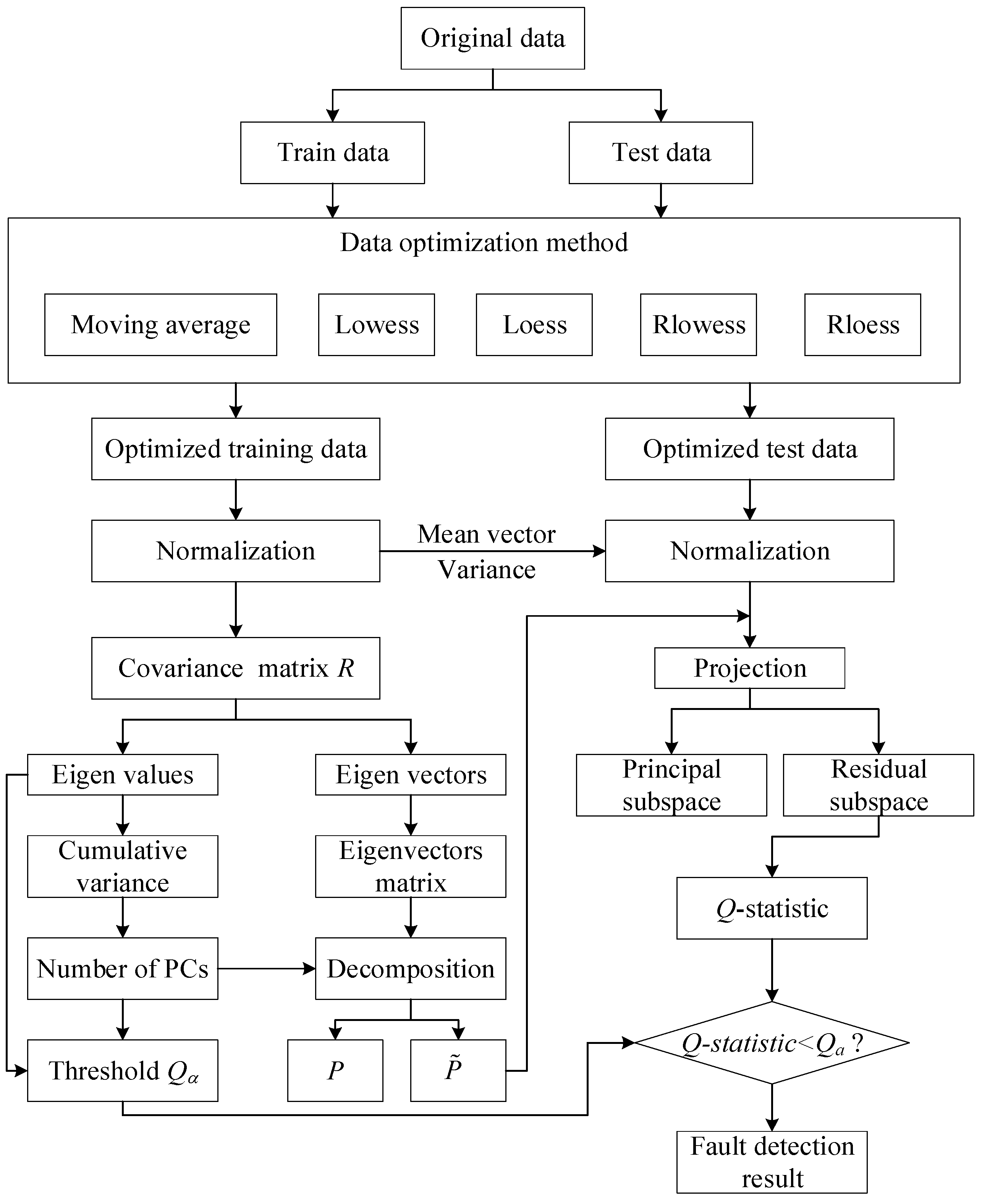
2.2. The PCA Method for Sensor Fault Detection

The principal component analysis approach is a multivariate statistical analysis technique and has been widely used in the field of sensor fault detection. The principal component analysis method mainly includes the following steps:

The data are normalized based on the mean and variance of each variable.

(1) The covariance matrix is calculated. X is the normalized data.

$$Cov\approx \frac{X^{T}X}{(n-1)}$$

(6)

(2) Eigenvalue decomposition is performed on the covariance matrix and arranged in descending order according to the size of the eigenvalue. The loading matrix $P\in R^{m\times k},P=\left[P_1\cdots P_k\right]$ is composed of the eigenvectors corresponding to the first k eigenvalues. The principal subspace is composed of vectors of P. Its orthogonal complement is the residual subspace $(I-P{P}^T)$. The choice of k value is determined by the cumulative contribution rate. The selection of k value in this study is based on the cumulative contribution rate exceeding 85%.

(3) The projection of the sample vector on the residual subspace is calculated.

$$\tilde{x}=(I-P{P}^T)x$$

(7)

(4) The Q-statistics is calculated. It measures the change in the projection of the sample vector in the residual space.

$$Q-statistic={\Vert (I-P{P}^T)x\Vert }^2\le Q_{\alpha }$$

(8)

(5) $Q_{\alpha }$ is the threshold of the Q-statistic, which can be determined statistically through the training matrix. Its calculation method is shown in Equation (9).

$$Q_{\alpha }={\theta }_1{\left[\frac{c_{\alpha }\sqrt{2{\theta }_2{h}_0^2}}{{\theta }_2}+1+\frac{{\theta }_2{h}_0(h_0-1)}{{\theta }_1^2}\right]}^{1/h_0}$$

(9)

where, $h_0=1-2{\theta }_1{\theta }_3/(3{\theta }_2^2)$, ${\theta }_t={\displaystyle \sum _{j=k+1}^m{\lambda }_j^t}$, t = 1, 2, 3. $\lambda$ is eigenvalues of the covariance matrix. When $\alpha$ = 5%, $c_{\alpha }$ = 1.645. $c_{\alpha }$ is standard normal distribution assigns confidence limits and α is confidence.

When there is no sensor fault, the Q-statistic is less than the threshold. Conversely, when the sensor occurs fault, the Q-statistic will be higher than the threshold.

3. Fault Detection Results of Optimized PCA Models

3.1. Data Set Description

The operating data of a chiller with a power of about 300 kW is selected to validate the proposed method. Both the evaporator and the condenser are full liquid shell and tube heat exchangers. The refrigerant is R134a and flows outside the heat exchanger tubes. The expansion valve is a thermal expansion valve. In addition to the refrigerant loop, the entire experimental system includes a chilled water loop, a cooling water loop, a hot water loop, a tap-water loop and a steam supply loop. The building heat load is simulated by steam and hot water loops. The condenser heat is taken away by tap water. In addition, a cooling water-chilled water heat exchanger between the condenser and the evaporator is used to assist in maintaining the cold and heat balance. There are 27 kinds of operating conditions during the experiment. The experiment system adjusted three parameters of evaporator outlet water temperature, condenser inlet water temperature and system cooling capacity. The control parameter setting values are listed in

Table 1. Setting values of control parameters under three operating conditions.

Variable	Evaporator Outlet Water Temperature (F)	Condenser Inlet Water Temperature (F)	Cooling Capacity (%)
Setting values	50	85	90–100
	45	75	70–80
	40	70	50–60
		65	25–40
		62	25–35
			45–50
			70–90

. A total of 64 variables were collected during the experiment. Among them, 48 variables are directly measured by the sensor, including variables such as temperature, pressure, flow, valve position, current, and power.

The sensor fault detection strategy proposed in this paper is validated by two normal working data sets. Each data set contains 4900 samples points, and the first set is used to train the model and the second set is used for testing. In order to establish the fault detection model based PCA method, 11 variables closely related to the system operation are selected to form the feature variable set of the PCA model, including evaporator inlet water temperature, evaporator outlet water temperature, condenser inlet water temperature, condenser outlet water temperature, cooling water flow, chilled water flow, evaporation saturation temperature, evaporation pressure, condensation saturation temperature, condensation pressure, and compressor discharge temperature. Sensor faults are introduced each time for a single variable.

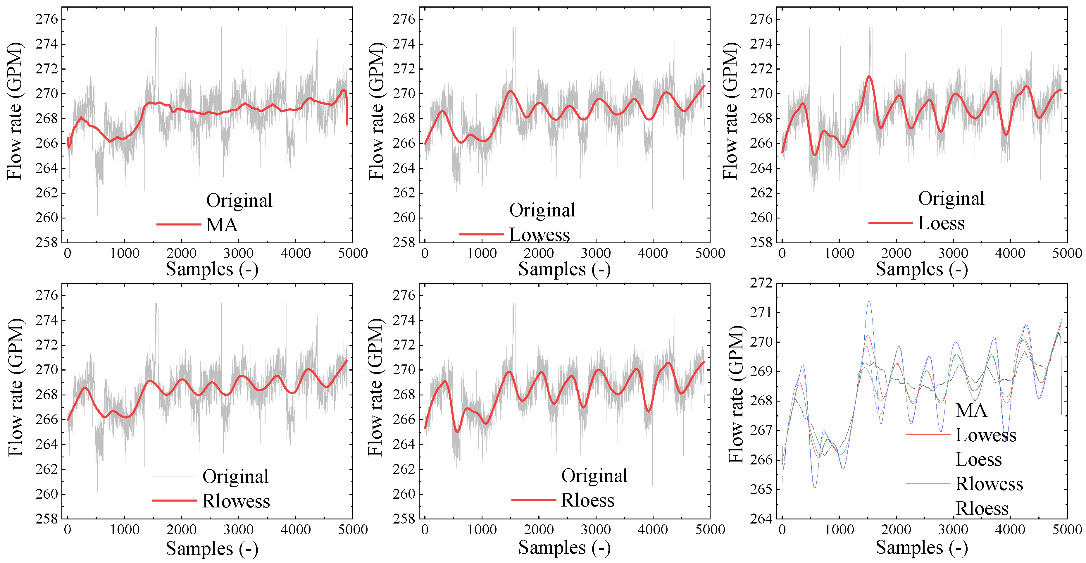
3.2. The Data Optimization Performance

The data smoothing methods need to set the span, and the span is the moving window width. The larger the span, the greater the smoothness. Therefore, four different smoothing levels are chosen in this paper. The parameter setting of span values of each data smoothing method are listed in

Table 2. Parameters sets of the span of different smooth approaches.

Smoothing Level	Different Approaches
	MA	Lowess	Loess	Rlowess	Rloess
Level 1	5	5	5	5	5
Level 2	9	10	10	10	10
Level 3	15	15	15	15	15
Level 4	19	20	20	20	20

. For the MA method, since the span must be an odd number, it is slightly different from other methods at level 2 and level 4.

Figure 3 shows the data optimization results for different data smoothing methods. The smoothing object in the figure is the running data of the cooling water flow, and the parameter is set to level 2. It can be seen from the figure that all of the five data smoothing algorithms have the smoothing effect on the original data, and the variability of the optimized data is significantly smaller than the original data. Meanwhile, it can also be seen from the area selected by the blue dotted box in the figure that data smoothing and denoising can effectively avoid obvious abnormal fluctuations. Besides, compared with these five different methods, it can be seen that the smoothing performance of the MA and Lowess methods is better than the other three methods. For the variable of cooling water flow, the data optimization of the Rloess method is poor.

In order to more intuitively compare the optimization performance of different data smoothing methods on the original data, Figure 4 shows the fluctuation of the optimized data. The fluctuation of the original data is very obvious, and there are many abnormal point fluctuations, as shown by the position of the red circles in the figure. For the optimized data, its variability is significantly reduced, and abnormal point fluctuations are reduced. Compared with different data optimization methods, the data optimization performance of MA method and Rlowess method is better. The variability is controlled within a range of ±1 and there is no obvious abnormal point fluctuation. The performance of Lowess method better than the Loess and Rloess methods. In addition, data variability in Loess method has improved. However, the optimized data still has many abnormal point fluctuations (as shown by the position of the black circles in the figure).

Different span settings will have a greater impact on the optimization of the original data. The MA method is used as an example to show the data optimization performance under four levels of smoothness, as shown in Figure 5. The span settings for the four levels of data smoothness are listed in Table 2. It can be seen from the figure that as the span setting increases, the smoothness of the data increases, and the variability of the data gradually decreases. At the same time, the optimized data still retains the trend of the original data. The graph of the fluctuation degree in Figure 5 reflects the degree of the fluctuation of the data. The smaller the value of the fluctuation degree, the more stable the data. When the span is set to level 3, the fluctuation degree of the data is in the range of ±1. On the other hand, the span setting is not as large as possible. Excessive parameters will make the data too smooth so that the optimized data information is lost and deviates from the original data.

3.3. Fault Detection Results

This section first discusses the establishment of the fault detection model and analyzes the Q-statistic of the training data set for different data optimization methods. Then the fault detection results of the three types of sensors are analyzed. Finally, the fault detection results under different data smoothness levels are compared and analyzed.

Figure 6 shows the results of the training set Q-statistic of the model established by various data optimization methods when the degree of smoothing is level 2. It can be seen from the figure that the fluctuation of the unoptimized model is obvious, and there are more sample points exceeding the threshold line. When the sensor fault detection models are optimized by five data smoothing methods, their Q-statistic fluctuations are alleviated. Among them, the optimization performance of Loess and Rloess methods is slightly worse than the other three methods. In addition, the optimized model has a significant fluctuation at the sample point of around 1500, and significantly exceeds the Q-statistic threshold. The reason for this is that there is an obvious data fluctuation in the point of the original data. This fluctuation information is retained after data optimization. The overall data are smoothed so that the Q-statistic of the established model at this point significantly exceeds the threshold line. Besides, by analyzing the threshold value of each model, it can be concluded that the threshold of the original data model is the largest, which is 4.16. The threshold of all of the optimized model has different degrees of reduction. The reduction of the Q-statistic threshold is beneficial to the model to detect a smaller degree of fault, and is beneficial to improve the performance of the fault detection model.

Table 3. Fault detection results of different types of sensors.

Fault Sensor	Fault Level	Fault Detection Model
		Original	MA	Lowess	Loess	Rlowess	Rloess
Evaporation temperature sensor	−7 °C	0.9996	1.0000	1.0000	1.0000	1.0000	0.9998
	−6 °C	0.8271	1.0000	1.0000	0.9898	1.0000	0.9906
	−5 °C	0.4298	0.9549	0.9078	0.6561	0.9259	0.6563
	−4 °C	0.2416	0.6600	0.5759	0.3953	0.5910	0.3867
	4 °C	0.1918	0.5100	0.4355	0.2882	0.4453	0.2920
	5 °C	0.3251	0.8396	0.7418	0.5012	0.7696	0.5027
	6 °C	0.6498	1.0000	0.9998	0.9322	1.0000	0.9333
	7 °C	0.9951	1.0000	1.0000	1.0000	1.0000	1.0000
Cooling water flow rate sensor	−6%	1.0000	1.0000	1.0000	1.0000	1.0000	1.0000
	−5%	0.9961	1.0000	1.0000	1.0000	1.0000	1.0000
	−4%	0.9914	0.9941	0.9937	0.9933	0.9935	0.9927
	−3%	0.9865	0.9910	0.9900	0.9892	0.9916	0.9898
	−2%	0.8539	0.9902	0.9884	0.9627	0.9910	0.9614
	−1%	0.2847	0.5947	0.5359	0.4090	0.5596	0.4057
	1%	0.2078	0.5849	0.5224	0.3622	0.5324	0.3547
	2%	0.7329	0.9824	0.9694	0.9212	0.9753	0.9186
	3%	0.9871	0.9978	0.9973	0.9969	0.9978	0.9967
	4%	0.9990	1.0000	1.0000	1.0000	1.0000	0.9998
	5%	0.9996	1.0000	1.0000	1.0000	1.0000	1.0000
	6%	1.0000	1.0000	1.0000	1.0000	1.0000	1.0000
Evaporation pressure sensor	−17%	0.8467	1.0000	0.9980	0.9690	0.9986	0.9690
	−16%	0.7088	0.9955	0.9865	0.9204	0.9884	0.9163
	−15%	0.5688	0.9814	0.9602	0.8208	0.9690	0.8149
	−14%	0.4484	0.9484	0.8935	0.6863	0.9059	0.6755
	−13%	0.3537	0.8590	0.7853	0.5561	0.8090	0.5400
	−12%	0.2884	0.7543	0.6612	0.4573	0.6867	0.4410
	12%	0.2241	0.5829	0.5045	0.3398	0.5169	0.3384
	13%	0.2712	0.6949	0.6114	0.4088	0.6286	0.4143
	14%	0.3388	0.8171	0.7294	0.5165	0.7559	0.5184
	15%	0.4249	0.9276	0.8627	0.6494	0.8859	0.6512
	16%	0.5504	0.9941	0.9606	0.7878	0.9745	0.7894
	17%	0.6914	1.0000	0.9992	0.9141	1.0000	0.9114

lists the fault detection results of the three sensors of evaporation temperature, cooling water flow rate and evaporation pressure, and the data optimization parameter is set to level 2. The fault detection performance of the model established after data optimization is better than the model established by the original data. From the overall results, the optimization performance of the MA method is better than the other four methods. Besides, Lowess and Rlowess methods are superior to Loess and Rloess methods. For example, when the cooling water flow rate sensor introduces a 2% deviation fault, the fault detection accuracy of the MA-PCA model is increased from 73.29% to 98.24%, and other optimization models are also improved. For the fault with evaporation temperature sensor deviation of 5 °C, the fault detection rate has increased from 32.51% to 83.96%, and the lifting effect is very obvious. These results also show that the improvement of the fault detection performance of the optimized PCA model is more obvious when the degree of sensor fault introduced is weak.

Figure 7 shows the fault detection performance of the various data optimization methods at different parameter settings when the fault is introduced into the cooling water flow sensor. When the ±1% fault is introduced, the fault detection performance of the MA, Lowess, and Rlowess methods is significantly improved, as shown by the red box in the figure. Besides, for the Loess and Rloess methods, when the data smoothness is level 1, the fault detection performance is slightly degraded. At the same time, the fault detection performance is improved at the other three levels, as shown in the blue box in the figure. When other degrees of the fault are introduced, the fault detection performance of the optimized PCA model is significantly improved. It can be seen from the results in the figure that as the smoothness of the data increases, the fault detection performance is better. Especially when the fault level is weak, the improvement of fault detection performance is more obvious with the smoothness is improved.

4. Discussions

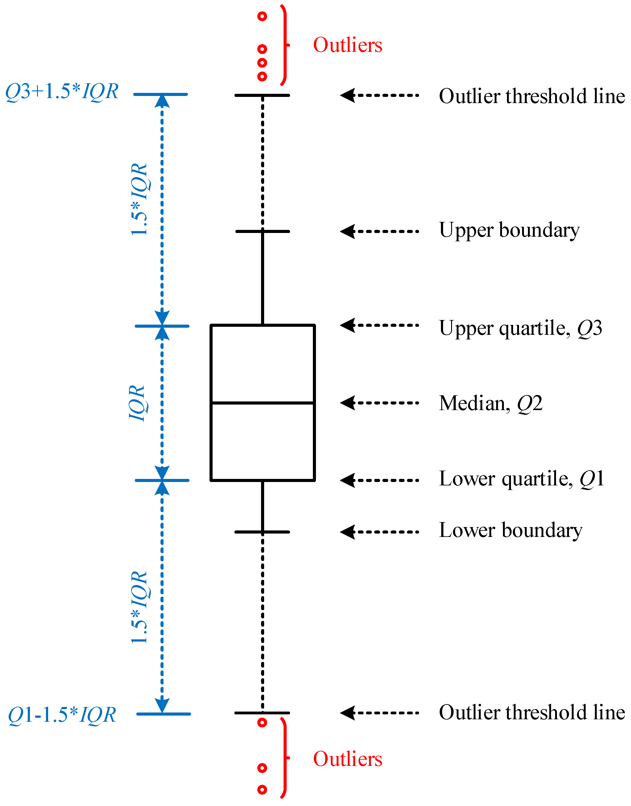
4.1. The Data Outlier Detection and Analysis

In order to more comprehensively analyze the data optimized by different methods, this section uses the outlier detection approach to evaluate different optimized data sets. Two representative outlier detection methods are selected, including the LOF method and the boxplot method.

The LOF method uses the local outlier factor size of the sample to measure the outlier degree of the sample, which is a relative density-based outlier detection algorithm based on the reachable distance. First, look for the first k neighbor sets of sample x and calculate the kth reachable distance of x to each neighbor sample.

$$r{d}_k(x,x^{(f)})=MAX\{d_k(x^{(k)}),d(x,x^{(f)})\}$$

(10)

where, $d_k(x^{(k)})$ is the distance between x and its kth nearest neighbor $d_k(x^{(k)})$. $d(x,x^{(f)})$ is the distance between x and its fth nearest neighbor $x^{(f)}$.

Second, calculate the local reachable density of sample x.

$$lr{d}_k(x)=\frac{1}{\frac{1}{k}{\displaystyle \sum _{f=1}^{k}r{d}_k(x,x^{(f)})}}$$

(11)

Finally, the local outlier factor of sample x is calculated.

$$LOF(x)=\frac{1}{k}{\displaystyle \sum _{f=1}^k\frac{lr{d}_k(x^{(f)})}{lr{d}_k(x)}}$$

(12)

The local outlier factor is close to 1, indicating that the sample x and its neighborhood point density are similar. In other words, x may belong to the same cluster as the neighborhood. If the local outlier factor is less than 1, the density of x is higher than the density of neighborhood points, which is a dense point. If the local outlier factor is larger than 1, it indicates that the density of x is less than its neighborhood point density. x may be an outlier. In this study, the LOF method is used to detect abnormal points of chiller operating data. To ensure the reliability of outlier detection, the threshold line for outlier determination is set to 1.5 That is, samples with a LOF factor larger than 1.5 are determined as outliers.

Boxplot is an approach to describe the data using five statistics, including the minimum value, upper quartile (Q1), median (Q2), lower quartile (Q3), and maximum value. Besides, IQR is the interval range. Boxplot can be used to identify data outliers, judge data skewness and tail weight. The schematic diagram of the boxplot method for outlier detection in this study is shown in Figure 8.

When the boxplot method is used to detect outliers, the threshold in this study is defined as follows.

$$l_{min}=Q_1-\beta \times IQR$$

(13)

$$l_{max}=Q_3+\beta \times IQR$$

(14)

where $\beta$ is set to 1.5 and IQR is the interval range Q3–Q1.

Figure 9 shows the results of the data optimized by different methods in this study using the two outlier detection methods. For the LOF method, it can be seen from the figure that except for the Loess method, the number of outliers has been reduced after data optimization. The degree of data fluctuation after optimization by the Loess method is reduced. However, it can also be seen from the results in Figure 4 that there are some abnormal samples relative to the optimized data. For the loess method, the data quality optimization effect is worse than other methods, so the number of abnormal samples increases after data optimization. Among them, the number of outliers detected from the data optimized by the Rlowess method is the smallest. For the boxplot method, the number of outliers after the data optimization of the Loess and Rloess methods increased, while the outliers of the other three methods decreased significantly. Comparing the two methods, it can be seen that the outlier number of data optimized by the Loess method increased. In connection with the previous section, the performance of the data optimization of Loess and Rloess methods is not as good as the other three methods. Therefore, the outlier detection results also explain the data optimization results and fault detection results of the previous sections. In addition, the number of outliers detected by the LOF method is higher than that of the boxplot method. In general, the number of outliers has decreased after data optimization.

4.2. The Parameter Selection of Data Smoothness

The previous section analyzed the performance of data optimization at different smoothing levels. As the degree of smoothing increases, the variability of the data decreases. However, when the parameter of span is set too large, the data may be too smooth, so that too much valid information is lost. In order to analyze the data processing results when the parameters of span are set too large, for the MA method, six levels of 99, 199, 299, 399, 499, and 599 are selected to smooth the data. The results are shown in Figure 10. It can be seen from the figure that when the parameter of span is set to 99, the trend of the smoothed is consistent with the original data. But when the parameter of span is 399, the smoothed data has begun to deviate from the original data. When the parameter of span reaches 599, the data is too smooth after data optimization and it is no longer possible to characterize the changing trend of the original data. The useful information of the original data is severely lost. This also illustrates that the data smoothing parameters can’t be set too large, and the parameter settings of span need to be on the premise of retaining valid information of the original data.

In order to comprehensively analyze the data smoothing performance when the parameter setting is too large, Figure 11 shows the data smoothing performance of the five optimized methods when the parameter is set to 499. It can be seen from the figure that, compared with other methods, the MA method has the most obvious deviation from the original data. When the parameter is set to 499, the data optimized by the other four methods still have a similar trend to the original data. Analyzing the results of these several methods, it can be found that when the parameter setting is large, the performance of the Lowess and Rlowess methods is consistent after data processing. At the same time, the Loess and Rloess methods have a similar phenomenon. Analyzing the data smoothing performance of the different methods, it is also concluded that the parameter setting can’t be too large. The data needs to be optimized while preserving valid information from the original data.

5. Conclusions

This study uses a variety of data optimization methods to optimize the sensor fault detection model for air conditioning systems. The research results will be of great help to building energy saving and emission reduction. The main conclusions are as follows:

(1)

The five smoothing methods have the effect of optimizing the data. The MA and Lowess methods are better than the other three methods. From the perspective of variability, the MA method has the best optimization performance when the smoothness degree is level 2. The optimized data fluctuation range is controlled within the range of ±1.

(2)

From the perspective of fault detection results, the Q-statistic threshold of the optimized PCA model is lower than that of the original model. Fault detection results have improved. Among them, when the evaporation temperature sensor fault is 5 °C deviation, the fault detection accuracy rate of the model optimized based on the MA method is increased from 32.51% to 83.96%, and the performance is significantly improved.

(3)

In addition, when the smoothing parameter is set too large, the data will deviate from the original data trend, and the effective information of the original data will be lost. Therefore, the smoothness of the data should not be too large.

Through data optimization and sensor fault detection research, it can be concluded that the MA method and Rlowess method are more suitable for data quality optimization in the field of air conditioning. Subsequent research will also use more abundant data to optimize the established model. In addition, the applicability of the proposed model to the data of different air-conditioning types such as air handling unit and variable refrigerant flow system will also be studied.

References

1. Hong, T.; Koo, C.; Kim, J.; Lee, M.; Jeong, K. A review on sustainable construction management strategies for monitoring, diagnosing, and retrofitting the building’s dynamic energy performance: Focused on the operation and maintenance phase. Appl. Energy 2015, 155, 671–707. [Google Scholar] [CrossRef]
2. Yang, L.; Yan, H.; Lam, J.C. Thermal comfort and building energy consumption implications–A review. Appl. Energy 2014, 115, 164–173. [Google Scholar] [CrossRef]
3. Yu, X.; Yan, D.; Sun, K.; Hong, T.; Zhu, D. Comparative study of the cooling energy performance of variable refrigerant flow systems and variable air volume systems in office buildings. Appl. Energy 2016, 183, 725–736. [Google Scholar] [CrossRef] [Green Version]
4. Guo, Y.; Chen, H. Fault diagnosis of VRF air-conditioning system based on improved Gaussian mixture model with PCA approach. Int. J. Refrig. 2020, 118, 1–11. [Google Scholar] [CrossRef]
5. Xu, Y.; Shen, C.; Lu, B.; Luo, C.; Wu, F.; Li, X.; Zhang, L. Study on the effect of NaBr modification on CaO-based sorbent for CO2 capture and SO2 capture. Carbon Cap. Sci. Technol. 2021, 1, 100015. [Google Scholar] [CrossRef]
6. Xu, Y.; Zhang, T.; Lu, B.; Luo, C.; Wu, F.; Li, X.; Zhang, L. Glycine tailored effective CaO-based heat carriers for thermochemical energy storage in concentrated solar power plants. Energ. Conver. Manag. 2021, 250, 114886. [Google Scholar] [CrossRef]
7. Xu, Y.; Lu, B.; Luo, C.; Wu, F.; Li, X.; Zhang, L. Na2CO3 promoted CaO-based heat carrier for thermochemical energy storage in concentrated solar power plants. Chem. Eng. J. 2022, 435, 134852. [Google Scholar] [CrossRef]
8. Lee, S.; Yik, F. A study on the energy penalty of various air-side system faults in buildings. Energy Build. 2010, 42, 2–10. [Google Scholar] [CrossRef]
9. Yoon, S.H.; Payne, W.V.; Domanski, P. Residential heat pump heating performance with single faults imposed. Appl. Therm. Eng. 2011, 31, 765–771. [Google Scholar] [CrossRef] [Green Version]
10. Hu, Y.; Li, G.; Chen, H.; Li, H.; Liu, J. Sensitivity analysis for PCA-based chiller sensor fault detection. Int. J. Refrig. 2016, 63, 133–143. [Google Scholar] [CrossRef]
11. Du, Z.; Chen, L.; Jin, X. Data-driven based reliability evaluation for measurements of sensors in a vapor compression system. Energy 2017, 122, 237–248. [Google Scholar] [CrossRef]
12. Han, H.; Gu, B.; Wang, T.; Li, Z. Important sensors for chiller fault detection and diagnosis (FDD) from the perspective of feature selection and machine learning. Int. J. Refrig. 2011, 34, 586–599. [Google Scholar] [CrossRef]
13. Elnour, M.; Meskin, N.; Al-Naemi, M. Sensor data validation and fault diagnosis using Auto-Associative Neural Network for HVAC systems. J. Build. Eng. 2019, 27, 100935. [Google Scholar] [CrossRef]
14. Guo, Y.; Wang, J.; Chen, H.; Li, G.; Huang, R.; Yuan, Y.; Ahmad, T.; Sun, S. An expert rule-based fault diagnosis strategy for variable refrigerant flow air conditioning systems. Appl. Therm. Eng. 2018, 149, 1223–1235. [Google Scholar] [CrossRef]
15. Wang, S.; Xing, J.; Jiang, Z.; Li, J. A decentralized sensor fault detection and self-repair method for HVAC systems. Build. Serv. Eng. Res. Technol. 2018, 39, 667–678. [Google Scholar] [CrossRef]
16. Shahnazari, H.; Mhaskar, P.; House, J.M.; Salsbury, T.I. Modeling and fault diagnosis design for HVAC systems using recurrent neural networks. Comput. Chem. Eng. 2019, 126, 189–203. [Google Scholar] [CrossRef]
17. Wang, S.; Xing, J.; Jiang, Z.; Dai, Y. A novel sensors fault detection and self-correction method for HVAC systems using decentralized swarm intelligence algorithm. Int. J. Refrig. 2019, 106, 54–65. [Google Scholar] [CrossRef]
18. Yan, R.; Ma, Z.; Kokogiannakis, G.; Zhao, Y. A sensor fault detection strategy for air handling units using cluster analysis. Autom. Constr. 2016, 70, 77–88. [Google Scholar] [CrossRef] [Green Version]
19. Li, G.; Hu, Y. Improved sensor fault detection, diagnosis and estimation for screw chillers using density-based clustering and principal component analysis. Energy Build. 2018, 173, 502–515. [Google Scholar] [CrossRef]
20. Montazeri, A.; Kargar, S.M. Fault detection and diagnosis in air handling using data-driven methods. J. Build. Eng. 2020, 31, 101388. [Google Scholar] [CrossRef]
21. Li, G.; Hu, Y.; Chen, H.; Li, H.; Hu, M.; Guo, Y.; Shi, S.; Hu, W. A sensor fault detection and diagnosis strategy for screw chiller system using support vector data description-based D-statistic and DV-contribution plots. Energy Build. 2016, 133, 230–245. [Google Scholar] [CrossRef]
22. Xu, X.; Xiao, F.; Wang, S. Enhanced chiller sensor fault detection, diagnosis and estimation using wavelet analysis and principal component analysis methods. Appl. Therm. Eng. 2008, 28, 226–237. [Google Scholar] [CrossRef]
23. Du, Z.; Fan, B.; Chi, J.; Jin, X. Sensor fault detection and its efficiency analysis in air handling unit using the combined neural networks. Energy Build. 2014, 72, 157–166. [Google Scholar] [CrossRef]
24. Zhao, Y.; Wen, J.; Xiao, F.; Yang, X.; Wang, S. Diagnostic Bayesian networks for diagnosing air handling units faults—Part I: Faults in dampers, fans, filters and sensors. Appl. Therm. Eng. 2017, 111, 1272–1286. [Google Scholar] [CrossRef]
25. Guo, Y.; Li, G.; Chen, H.; Hu, Y.; Li, H.; Xing, L.; Hu, W. An enhanced PCA method with Savitzky-Golay method for VRF system sensor fault detection and diagnosis. Energy Build. 2017, 142, 167–178. [Google Scholar] [CrossRef]
26. Kocyigit, N. Fault and sensor error diagnostic strategies for a vapor compression refrigeration system by using fuzzy inference systems and artificial neural network. Int. J. Refrig. 2015, 50, 69–79. [Google Scholar] [CrossRef]
27. Li, S.; Wen, J. A model-based fault detection and diagnostic methodology based on PCA method and wavelet transform. Energy Build. 2014, 68, 63–71. [Google Scholar] [CrossRef]
28. Zhu, Y.; Jin, X.; Du, Z. Fault diagnosis for sensors in air handling unit based on neural network pre-processed by wavelet and fractal. Energy Build. 2012, 44, 7–16. [Google Scholar] [CrossRef]
29. Li, G.; Hu, Y. An enhanced PCA-based chiller sensor fault detection method using ensemble empirical mode decomposition based denoising. Energy Build. 2018, 183, 311–324. [Google Scholar] [CrossRef]
30. Yalcin, O.F.; Dicleli, M. Effect of the high frequency components of near-fault ground motions on the response of linear and nonlinear SDOF systems: A moving average filtering approach. Soil Dyn. Earthq. Eng. 2020, 129. [Google Scholar] [CrossRef]
31. Mariani, M.; Basu, K. Local regression type methods applied to the study of geophysics and high frequency financial data. Phys. A Stat. Mech. Its Appl. 2014, 410, 609–622. [Google Scholar] [CrossRef]
Figure 1. Schematic diagram of principal component analysis fault detection strategy optimized using multiple data smoothing methods.
Processes 10 00347 g001
Figure 2. Data smoothing diagram of the moving average method.
Processes 10 00347 g002
Figure 3. Data optimization results of cooling water flow rate for different data smoothing methods.
Processes 10 00347 g003
Figure 4. The data fluctuation of the cooling water flow sensor optimized by different methods when the smoothing level is level 2.
Processes 10 00347 g004
Figure 5. Data quality optimization performance of the MA method with different parameter settings.
Processes 10 00347 g005
Figure 6. Q-statistics results of training data set for different data optimization methods.
Processes 10 00347 g006
Figure 7. Fault detection results of different optimized PCA models for the cooling water flow sensor.
Processes 10 00347 g007
Figure 8. Schematic diagram of outlier detection using boxplot method.
Processes 10 00347 g008
Figure 9. Outlier detection results of the different methods.
Processes 10 00347 g009
Figure 10. Data smoothing results when the parameter of the MA method is set too large.
Processes 10 00347 g010
Figure 11. Data smoothing results of the different methods when the parameter is set too large.
Processes 10 00347 g011