Article

On the Laplace Transforms of the First Hitting Times for Drawdowns and Drawups of Diffusion-Type Processes

by
Pavel V. Gapeev
1,*,
Neofytos Rodosthenous
2 and
V. L. Raju Chinthalapati
3
1
Department of Mathematics, London School of Economics, Houghton Street, London WC2A 2AE, UK
2
School of Mathematical Sciences, Queen Mary University of London, Mile End Road, London E1 4NS, UK
3
Southampton Business School, University of Southampton, Southampton SO17 1BJ, UK
*
Author to whom correspondence should be addressed.
Risks 2019, 7(3), 87; https://doi.org/10.3390/risks7030087
Submission received: 27 May 2019 / Revised: 18 July 2019 / Accepted: 30 July 2019 / Published: 5 August 2019

Abstract

:
We obtain closed-form expressions for the value of the joint Laplace transform of the running maximum and minimum of a diffusion-type process stopped at the first time at which the associated drawdown or drawup process hits a constant level before an independent exponential random time. It is assumed that the coefficients of the diffusion-type process are regular functions of the current values of its running maximum and minimum. The proof is based on the solution to the equivalent inhomogeneous ordinary differential boundary-value problem and the application of the normal-reflection conditions for the value function at the edges of the state space of the resulting three-dimensional Markov process. The result is related to the computation of probability characteristics of the take-profit and stop-loss values of a market trader during a given time period.

1. Introduction

The aim of this paper is to derive closed-form expressions for the joint Laplace transform (4) of the first time to a fixed drawdown occurring before a fixed drawup of the diffusion-type process X and its running maximum and minimum S and Q defined in (1)–(2) considered up to a random exponentially distributed time η , which is independent of the driving standard Brownian motion. We consider a model for the diffusion-type process X with the coefficients being regular functions of the current values of the process X itself as well as of its running maximum and minimum S and Q. The value function in (4) provides the Laplace transform of the value function in (6) which is the joint Laplace transform of the same random variables representing functionals of the diffusion-type process X stopped before a fixed time. We derive a closed-form solution to the equivalent inhomogeneous ordinary differential boundary-value problem for the value of the joint Laplace transform as a stopping problem for the resulting three-dimensional continuous Markov process ( X , S , Q ) . This result can therefore be interpreted as the computation of the probability characteristics of the random variables associated with the take-profit and stop-loss values of a market trader on a fixed-time interval. The problem of computation of the Laplace transform of the same random times and variables in a model in which the coefficients of the original diffusion-type process depend on the current values of the running maximum and minimum as well as on the maximum drawdown and maximum drawup was explicitly solved in Gapeev and Rodosthenous (2015) on the infinite time interval. Other functionals of diffusion processes evaluated at independent exponential times were computed in Borodin and Salminen (Borodin and Salminen 2002, Part II) among others.
The joint Laplace transform of the first time at which a Brownian motion with linear drift hits a given drawdown value and the running maximum stopped at the same time was computed by Taylor (1975). The joint distribution of the same random variables was obtained by Lehoczky (1977). The mean value and the density of the maximum drawdown of a Brownian motion with linear drift were explicitly derived by (Douady et al. 2000; Magdon-Ismail et al. 2004), respectively. More recently, Pospisil et al. (2009) computed the probability of the event that the drawdown of a one-dimensional diffusion reaches a fixed value occurs before the drawup of the same process reaches another fixed value. Mijatović and Pistorius (2012) obtained the distribution laws of the first-passage times of spectrally positive and negative Lévy processes over constant levels and derived explicit expressions for several related characteristics for the drawdowns and drawups in those models. An extensive overview of various probabilistic and practically applied aspects of drawdowns such as the speed of market crashes and others was recently provided in the monograph of Zhang (2018).
The diffusion-type processes can be considered as immediate generalisations of the diffusion processes particularly arising in the so-called local volatility models introduced by Dupire (1997), where the local drift and diffusion coefficients depend only on the running value of the original process. Other generalisations of the original processes with diffusion coefficients depending on the running values of the initial processes and their running minima were constructed by Forde (2011) for given joint laws of the terminal level and supremum at an independent exponential time (see also Forde et al. 2013; Zhang 2014) for other important probability characteristics of processes of such type). The valuation functional equations for general functional path-dependent volatility models were derived in (Cont and Fournié 2013; Fournié 2010), who also considered the sensitivity analysis of path-dependent financial derivative securities. Henry-Labordère (2009) and Ren et al. (2007), among others, considered the option pricing and calibration problems in models of stochastic interest rates and volatility based on diffusion-type processes with tractable path-dependent coefficients.
Optimal stopping problems for running maxima of some diffusion processes were studied by (Jacka 1991; Dubins et al. 1993; Peskir 1998; Peskir and Shiryaev 2006, chp. V) among others. Discounted optimal stopping problems for certain payoff functions depending on the current values of the running maxima of geometric Brownian motions were initiated by (Shepp and Shiryaev 1993, 1994) and then taken further by (Pedersen 2000; Guo and Shepp 2001; Guo and Zervos 2010, Glover et al. 2013; Rodosthenous and Zervos 2017) among others. Moreover, Peskir (2012, 2014) studied optimal stopping problems for three-dimensional Markov processes having the initial diffusion process as well as its maximum and minimum as state space components. Other three-dimensional optimal stopping problems for continuous Markov processes of such type were studied in (Gapeev and Rodosthenous 2014, 2016) among others. The main feature of the resulting optimal stopping problems and their equivalent free-boundary problems was the application of the normal-reflection conditions for the value functions at the edges of the multi-dimensional state spaces to derive systems of first-order nonlinear ordinary differential equations for the optimal stopping boundaries depending on the current values of the running extremal processes. Optimal stopping problems for diffusion and spectrally negative Lévy processes on random time intervals were considered in (Carr 1998; Avram et al. 2004; Agarwal et al. 2016) among others. It turned out that the resulting value functions and optimal stopping boundaries in models with exponentially distributed time horizons independent of the underlying processes are analytically more tractable than those obtained in models with fixed time horizons. Other optimal stopping problems for exponentially distributed time horizons which are dependent of the underlying Lévy process were recently considered in Rodosthenous and Zhang (2018).
Glattfelder et al. (2011) suggested a new paradigm, the directional changes, that summarises the price dynamics in the financial market. Unlike interval based summary along the physical time, the new paradigm summarizes the price movements along the intrinsic time scale of the market that is driven by the events in the market. The events in the market are identified by the a priori defined significant percentage of price moves known as thresholds. For a given threshold, the price movements are summarised by identifying the local price extremes from where there has been a percentage drop (or rise) in price that accedes the threshold. The process of price drop (or rise) from a local price extreme to the point where the price is dropped (risen) by the threshold is defined as directional change event. The price movement that continues after directional change event in the same direction beyond the threshold is considered as overshoot. Roughly speaking, directional changes and overshoots summarise the upward or downward trends in the market according to the prescribed thresholds. It is obvious that the summary of the directional changes is depending on the selected threshold. Using the high frequency foreign exchange data, in Glattfelder et al. (2011) scaling laws were demonstrated in intrinsic times for the variables like average times that are taken for directional changes, event thresholds, average overshoots, etc. The authors of Glattfelder et al. (2011) have identified 12 scaling laws across 13 currency pairs that are consistent over varying time intervals. The scaling laws throw light on market physics of moving prices. Each scaling law encapsulates certain stylised facts of the market. The scaling law that describes the relationship between the directional change and overshoot sections of the total price move has drawn quite a lot of attention. Even though the empirical evidence of the scaling laws is demonstrated in the literature (see, e.g., Bakhach et al. 2018; Bakhach et al. 2018; Tsang et al. 2017), the required theoretical framework is not developed yet. We believe that the present work on first hitting times for drawdowns and drawups on diffusion-type processes on random time horizons throws light on the underlying theoretical aspects of the scaling laws that are presented in financial data.
The paper is organised as follows. In Section 2, we introduce the setting and notation of the model with a three-dimensional continuous Markov process, whose state space components are the original process and its running maximum and minimum processes. We define the value function of the joint Laplace transform of the first time to a fixed drawdown occurring before the first time of a fixed drawup and an independent exponential time together with the running maximum and minimum processes stopped at the earliest of those times. In Section 3, we obtain a closed-form solution to the associated inhomogeneous ordinary differential boundary-value problem and show that the value function represents a linear combination of the solutions to the systems of first-order partial differential equations which arise from the application of the normal-reflection conditions for this function at the edges of the three-dimensional state space. We also illustrate the results on several examples of the original processes representing locally a Brownian motion with drift, or a mean-reverting Ornstein-Uhlenbeck process, or the logarithm of a Feller square root process. In Section 4, we formulate the result of the paper and prove that the solution to the boundary-value problem provides the required joint Laplace transform.

2. Preliminaries

In this section, we give a precise formulation of the model and the three-dimensional stopping problem as well as its equivalent boundary-value problem.

2.1. Formulation of the Problem

Let us consider a probability space ( Ω , F , P ) with a standard Brownian motion B = ( B t ) t 0 and a positive random time η such that P ( η > t ) = e α t , for all t 0 and some α > 0 fixed (B and η are supposed to be independent). Assume that there exists a process X = ( X t ) t 0 solving the stochastic differential equation
d X t = μ ( X t , S t , Q t ) d t + σ ( X t , S t , Q t ) d B t ( X 0 = x )
where x R is fixed, and μ ( x , s , q ) and σ ( x , s , q ) > 0 are continuously differentiable functions on [ , ] 3 which are of at most linear growth in x and uniformly bounded in s and q. Here, the associated with X running maximum process S = ( S t ) t 0 and the running minimum process Q = ( Q t ) t 0 are defined by
S t = s max 0 u t X u and Q t = q min 0 u t X u
for arbitrary q x s . It follows from the result of (Liptser and Shiryaev [1977] 2001, chp. IV, Theorem 4.8) that the equation in (1) admits a pathwise unique (strong) solution. We also define the associated first hitting (stopping) times
τ a = inf { t 0 | S t X t a } and ζ b = inf { t 0 | X t Q t b }
for some a , b > 0 fixed.
The purpose of the present paper is to derive closed-form expressions for the joint Laplace transform of the random time τ a ζ b η and the random variables S τ a ζ b η and Q τ a ζ b η . We therefore need to compute the value function of the following stopping problem for the (time-homogeneous strong) Markov process ( X , S , Q ) = ( X t , S t , Q t ) t 0 given by
V * ( x , s , q ) = E x , s , q [ e λ ( τ a η ) θ S τ a η κ Q τ a η I ( τ a < ζ b ) ]
for any ( x , s , q ) E 3 and some λ , θ , κ > 0 fixed, where I ( · ) denotes the indicator function. Here, E x , s , q denotes the expectation under the assumption that the (three-dimensional) Markov process ( X , S , Q ) defined in (1)–(2) starts at ( x , s , q ) E 3 , where we assume that the state space of ( X , S , Q ) is essentially E 3 = { ( x , s , q ) R 3 | q x s } with its border planes d 1 3 = { ( x , s , q ) R 3 | x = s } and d 2 3 = { ( x , s , q ) R 3 | x = q } .
It follows from the independence of the process X and the random time η that the value function in (4) admits the representation
V * ( x , s , q ) = 0 W * ( T ; x , s , q ) α e α T d T
where we set
W * ( T ; x , s , q ) = E x , s , q [ e λ ( τ a T ) θ S τ a T κ Q τ a T I ( τ a < ζ b ) ]
for any ( x , s , q ) E 3 , and each T > 0 fixed.

2.2. The Boundary-Value Problems

By means of standard arguments based on the application of Itô’s formula (see, e.g., Karatzas and Shreve 1991, chp. V, sct. 5.1), it is shown that the infinitesimal operator L of the process ( X , S , Q ) acts on a function F ( x , s , q ) from the class C 2 , 1 , 1 on the interior of E 3 according to the rule
( L F ) ( x , s , q ) = μ ( x , s , q ) x F ( x , s , q ) + σ 2 ( x , s , q ) 2 x x F ( x , s , q )
for all q < x < s . It follows from the results of general theory of Markov processes (see, e.g., Dynkin 1965, chp. V) that the value function W * ( T ; x , s , q ) in (6) solves the equivalent parabolic-type boundary-value problem
( L W λ W T W ) ( T ; x , s , q ) = 0 for ( s a ) q < x < s ( q + b )
W ( T ; x , s , q ) | x = ( s a ) + = e θ s κ q for s q a
W ( T ; x , s , q ) | x = ( q + b ) = 0 for s q b
q W ( T ; x , s , q ) | x = q + = 0 for 0 < s q < a
s W ( T ; x , s , q ) | x = s = 0 for 0 < s q < b
for all T > 0 . In this case, using the integration-by-parts formula, and taking into account the assumption that the value function in (6) is bounded, we have
0 T W ( T ; x , s , q ) α e α T d T = W ( T ; x , s , q ) α e α T 0 + 0 W ( T ; x , s , q ) α 2 e α T d T = α e θ s κ q + 0 W ( T ; x , s , q ) α 2 e α T d T = α e θ s κ q + α V ( x , s , q )
0 x W ( T ; x , s , q ) α e α T d T = x V ( x , s , q )
0 x x W ( T ; x , s , q ) α e α T d T = x x V ( x , s , q )
0 q W ( T ; x , s , q ) α e α T d T = q V ( x , s , q )
and
0 s W ( T ; x , s , q ) α e α T d T = s V ( x , s , q )
for all ( x , s , q ) E 3 . Hence, it follows from the boundary-value problem in (8)–(12), that the value function V * ( x , s , q ) in (6) solves the equivalent inhomogeneous ordinary boundary-value problem
( L V ( α + λ ) V ) ( x , s , q ) = α e θ s κ q for ( s a ) q < x < s ( q + b )
V ( x , s , q ) | x = ( s a ) + = e θ s κ q for s q a
V ( x , s , q ) | x = ( q + b ) = 0 for s q b
q V ( x , s , q ) | x = q + = 0 for 0 < s q < a
s V ( x , s , q ) | x = s = 0 for 0 < s q < b
for a , b > 0 fixed. Note that the homogeneous version of the ordinary differential boundary-value problem in (18)–(22) in a model with more general diffusion-type processes X was explicitly solved in (Gapeev and Rodosthenous 2015, sct. 3).

3. Solutions to the Boundary-Value Problem

In this section, we obtain closed-form solutions to the boundary-value problem in (18)–(22) under various relations on the parameters of the model.

3.1. The General Solution of the Ordinary Differential Equation

We first observe that the general solution of the equation in (18) has the form
V ( x , s , q ) = C 1 ( s , q ) Ψ 1 ( x , s , q ) + C 2 ( s , q ) Ψ 2 ( x , s , q ) + α α + λ e θ s κ q
where C i ( s , q ) , i = 1 , 2 , are some arbitrary continuously differentiable functions, and Ψ i ( x , s , q ) , i = 1 , 2 , are the two fundamental positive solutions (i.e., nontrivial linearly independent particular solutions) of the homogeneous version of the second-order ordinary differential equation in (18). Without loss of generality, we may assume that Ψ 1 ( x , s , q ) and Ψ 2 ( x , s , q ) are the (strictly) increasing and decreasing (convex) functions, respectively. Note that these solutions should satisfy the properties Ψ 1 ( r , r , r ) and Ψ 2 ( r , r , r ) 0 as r and Ψ 1 ( r , r , r ) 0 and Ψ 2 ( r , r , r ) as r on the state space E 3 of the process ( X , S , Q ) . These functions can be represented as the functionals
Ψ 1 ( x , s , q ) = E x , s , q [ e λ ξ I ( ξ < ) ] , if x x 1 / E x , s , q [ e λ ξ I ( ξ < ) ] , if x x
and
Ψ 2 ( x , s , q ) = 1 / E x , s , q [ e λ ξ I ( ξ < ) ] , if x x E x , s , q [ e λ ξ I ( ξ < ) ] , if x x
of the first hitting times ξ = inf { t 0 | X t = x } and ξ = inf { t 0 | X t = x } of the process X solving the stochastic differential equation in (1) and started at x and x such that ( x , s , q ) , ( x , s , q ) E 3 , respectively (see, e.g., Rogers and Williams 1987, chp. V, sct. 50 for further details).
Hence, by applying the conditions of (19)–(22) to the function in (23), we obtain the equalities
C 1 ( s , q ) Ψ 1 ( s a , s , q ) + C 2 ( s , q ) Ψ 2 ( s a , s , q ) = λ α + λ e θ s κ q
for s q a ,
C 1 ( s , q ) Ψ 1 ( q + b , s , q ) + C 2 ( s , q ) Ψ 2 ( q + b , s , q ) = α α + λ e θ s κ q
for s q b ,
i = 1 2 q C i ( s , q ) Ψ i ( q , s , q ) + C i ( s , q ) q Ψ i ( x , s , q ) | x = q = α κ α + λ e θ s κ q
for 0 < s q < a ,
i = 1 2 s C i ( s , q ) Ψ i ( s , s , q ) + C i ( s , q ) s s Ψ i ( x , s , q ) | x = s = α θ α + λ e θ s κ q
for 0 < s q < b .

3.2. The Solution to the Boundary-Value Problem

We now derive the solution of the boundary-value problem in (18)–(22). For this purpose, we recall that the second and third components of the process ( X , S , Q ) can increase and decrease only at the planes d 1 3 and d 2 3 , that is, when X t = S t and X t = Q t for t 0 , respectively.
(i) Let us first consider the domain a b s q a + b . In this case, solving the system of equations in (26) and (27), we conclude that the candidate value function admits the representation
V ( x , s , q ; ) = C 1 ( s , q ; ) Ψ 1 ( x , s , q ) + C 2 ( s , q ; ) Ψ 2 ( x , s , q ) + α α + λ e θ s κ q
in the region R 3 ( ) = { ( x , s , q ) E 3 | q s a x q + b s } , with
C 1 ( s , q ; ) = e θ s κ q ( λ Ψ 2 ( q + b , s , q ) + α Ψ 2 ( s a , s , q ) ) / ( α + λ ) Ψ 1 ( s a , s , q ) Ψ 2 ( q + b , s , q ) Ψ 1 ( q + b , s , q ) Ψ 2 ( s a , s , q )
and
C 2 ( s , q ; ) = e θ s κ q ( λ Ψ 1 ( q + b , s , q ) + α Ψ 1 ( s a , s , q ) ) / ( α + λ ) Ψ 1 ( q + b , s , q ) Ψ 2 ( s a , s , q ) Ψ 1 ( s a , s , q ) Ψ 2 ( q + b , s , q )
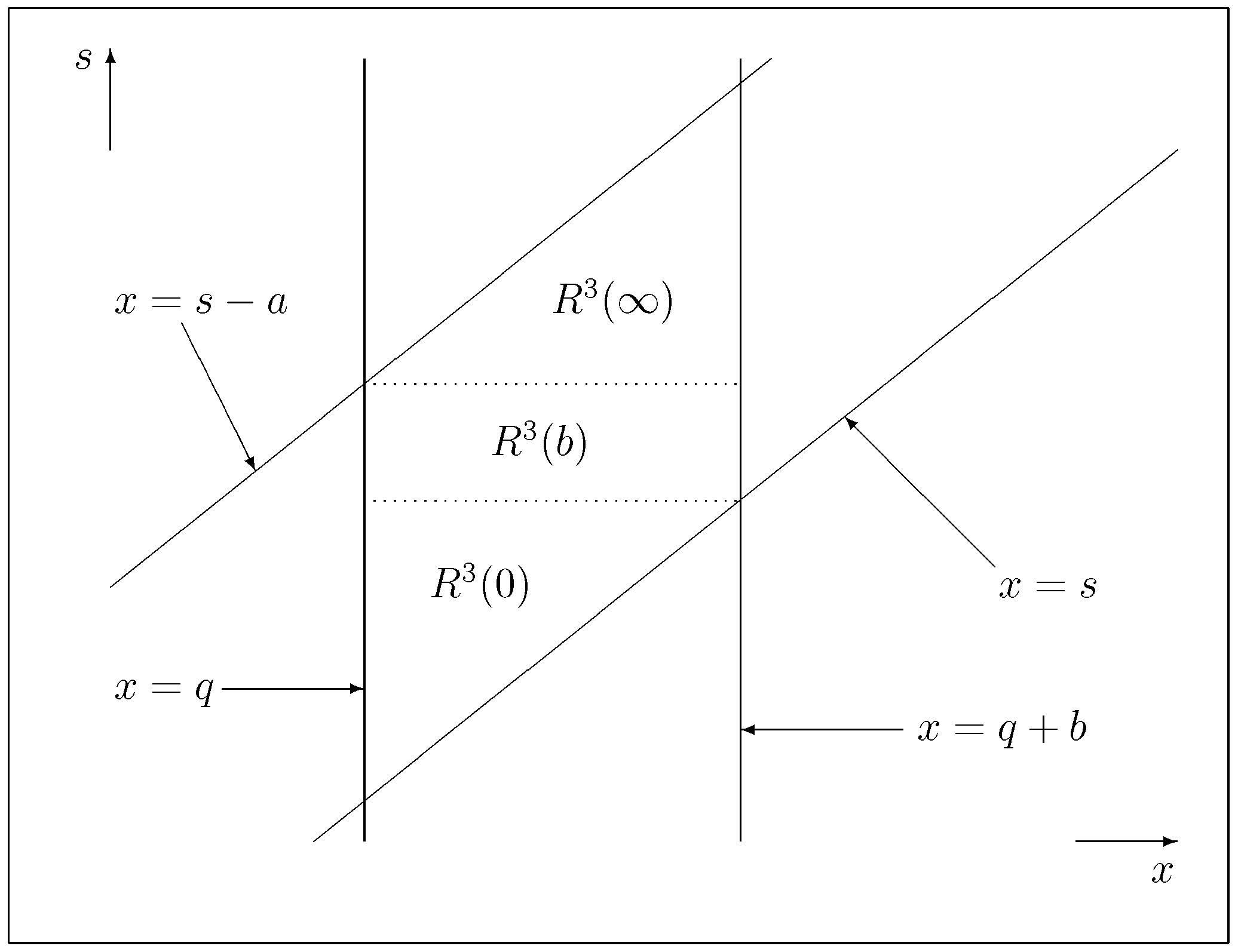
for all q + a b s q + a + b (see Figure 1 and Figure 2 below).
(ii) Let us now consider the domain a s q < b . In this case, it follows from the equations in (26) and (29) that the candidate value function admits the representation
V ( x , s , q ; a ) = C 1 ( s , q ; a ) Ψ 1 ( x , s , q ) + C 2 ( s , q ; a ) Ψ 2 ( x , s , q ) + α α + λ e θ s κ q
in the region R 3 ( a ) = { ( x , s , q ) E 3 | q s a x s < q + b } , with
C 2 ( s , q ; a ) = λ α + λ e θ s κ q Ψ 2 ( s a , s , q ) C 1 ( s , q ; a ) Ψ 1 ( s a , s , q ) Ψ 2 ( s a , s , q )
for q + a s < q + b , where C 1 ( s , q ; a ) solves the first-order linear ordinary differential equation
s C 1 ( s , q ; a ) H 1 , 2 ( s , q ; a ) + C 1 ( s , q ; a ) H 1 , 1 ( s , q ; a ) = H 1 , 0 ( s , q ; a )
with
H 1 , 2 ( s , q ; a ) = Ψ 1 ( s , s , q ) Ψ 2 ( s , s , q ) Ψ 1 ( s a , s , q ) Ψ 2 ( s a , s , q )
H 1 , 1 ( s , q ; a ) = s Ψ 1 ( x , s , q ) | x = s H 1 , 1 ( s , q ; a ) = s Ψ 1 ( s a , s , q ) Ψ 2 ( s a , s , q ) Ψ 2 ( s , s , q ) Ψ 1 ( s a , s , q ) Ψ 2 ( s a , s , q ) s Ψ 1 ( x , s , q ) | x = s
H 1 , 0 ( s , q ; a ) = λ α + λ ( θ e θ s κ q H 1 , 0 ( s , q ; a ) = s e θ s κ q Ψ 2 ( s a , s , q ) Ψ 2 ( s , s , q ) e θ s κ q Ψ 2 ( s a , s , q ) s Ψ 2 ( x , s , q ) | x = s )
for all q + a s < q + b . Observe that the process ( X , S , Q ) can exit the region R 3 ( a ) by passing to the region R 3 ( ) in part (i) of this subsection only through the point x = s = q + b , by hitting the plane d 1 3 so that increasing its second component S. Thus, the candidate function V ( x , s , q ) should be continuous at the point ( q + b , q + b , q ) , that is expressed by the equality
C 1 ( q + b , q ; a ) Ψ 1 ( q + b , q + b , q ) + C 2 ( q + b , q ; a ) Ψ 2 ( q + b , q + b , q ) = α α + λ e θ ( q + b ) κ q
for all q R (see Figure 1 above). Hence, solving the differential equation in (35) together with the system of equations in (34) with s = q + b and (39), we obtain
C 1 ( s , q ; a ) = C 1 ( q + b , q ; a ) exp s q + b H 1 , 1 ( u , q ; a ) H 1 , 2 ( u , q ; a ) d u = s q + b H 1 , 0 ( u , q ; a ) H 1 , 2 ( u , q ; a ) exp s u H 1 , 1 ( v , q ; a ) H 1 , 2 ( v , q ; a ) d v d u
for all q + a s < q + b , where C 1 ( q + b , q ; a ) is given by
C 1 ( q + b , q ; a ) = e θ ( q + b ) κ q ( λ Ψ 2 ( q + b , q + b , q ) + α Ψ 2 ( q + b a , q + b , q ) ) / ( α + λ ) Ψ 1 ( q + b a , q + b , q ) Ψ 2 ( q + b , q + b , q ) Ψ 1 ( q + b , q + b , q ) Ψ 2 ( q + b a , q + b , q )
for all q R .
Note that in the case in which μ ( s , q ) = μ ( s ) and σ ( s , q ) = σ ( s ) in (1) as well as κ = 0 and b = in (6), the candidate value function admits the representation of (33) with V ( x , s , q ; a ) = U ( x , s ; a ) and C i ( s , q ; a ) = D i ( s ; a ) as well as Ψ i ( x , s , q ) = Φ i ( x , s ) , i = 1 , 2 . Moreover, we observe that D 1 ( ; a ) = 0 should hold in (33), since otherwise U ( x , s ; a ) ± as x = s , which must be excluded, by virtue of the obvious fact that the value function V * ( x , s , q ) = U * ( x , s ) in (6) is bounded. Therefore, using arguments similar to the ones above, we conclude that the function C 2 ( s , q ; a ) = D 2 ( s ; a ) has the form of (34) with C 1 ( s , q ; a ) = D 1 ( s ; a ) given by
D 1 ( s ; a ) = s G 1 , 0 ( u ; ) G 1 , 2 ( u ; ) exp s u G 1 , 1 ( v ; ) G 1 , 2 ( v ; ) d v d u
and H 1 , j ( s , q ; a ) = G 1 , j ( s ; a ) , j = 0 , 1 , 2 , from (36)–(38), for all s R .
(iii) Let us now consider the domain b s q < a . In this case, it follows from the equations in (27) and (28) that the candidate value function admits the representation
V ( x , s , q ; b ) = C 1 ( s , q ; b ) Ψ 1 ( x , s , q ) + C 2 ( s , q ; b ) Ψ 2 ( x , s , q ) + α α + λ e θ s κ q
in the region R 3 ( b ) = { ( x , s , q ) E 3 | s a < q x q + b s } , with
C 2 ( s , q ; b ) = α α + λ e θ s κ q Ψ 2 ( q + b , s , q ) C 1 ( s , q ; b ) Ψ 1 ( q + b , s , q ) Ψ 2 ( q + b , s , q )
for q + b s < q + a , where C 1 ( s , q ; b ) solves the first-order linear ordinary differential equation
q C 1 ( s , q ; b ) H 2 , 2 ( s , q ; b ) + C 1 ( s , q ; b ) H 2 , 1 ( s , q ; b ) = H 2 , 0 ( s , q ; b )
with
H 2 , 2 ( s , q ; b ) = Ψ 1 ( q , s , q ) Ψ 2 ( q , s , q ) Ψ 1 ( q + b , s , q ) Ψ 2 ( q + b , s , q )
H 2 , 1 ( s , q ; b ) = q Ψ 1 ( x , s , q ) | x = q q Ψ 1 ( q + b , s , q ) Ψ 2 ( q + b , s , q ) Ψ 2 ( q , s , q ) Ψ 1 ( q + b , s , q ) Ψ 2 ( q + b , s , q ) q Ψ 2 ( x , s , q ) | x = q
H 2 , 0 ( s , q ; b ) = α α + λ ( κ e θ s κ q + q e θ s κ q Ψ 2 ( q + b , s , q ) Ψ 2 ( q , s , q ) + e θ s κ q Ψ 2 ( q + b , s , q ) q Ψ 2 ( x , s , q ) | x = q )
for all q + b s < q + a . Observe that the process ( X , S , Q ) can exit R 3 ( b ) by passing to the region R 3 ( ) in part (i) of this subsection only through the point x = q = s a , by hitting the plane d 2 3 so that decreasing its third component Q. Then, the candidate value function should be continuous at the point ( s a , s , s a ) , that is expressed by the equality
C 1 ( s , s a ; b ) Ψ 1 ( s a , s , s a ) + C 2 ( s , s a ; b ) Ψ 2 ( s a , s , s a ) = α α + λ e θ s κ ( s a )
for all s R (see Figure 2 below). Hence, solving the differential equation in (45) together with the system of equations in (44) with q = s a and (49), we obtain
C 1 ( s , q ; b ) = C 1 ( s , s a ; b ) exp s a q H 2 , 1 ( s , u ; b ) H 2 , 2 ( s , u ; b ) d u = + s a q H 2 , 0 ( s , u ; b ) H 2 , 2 ( s , u ; b ) exp u q H 2 , 1 ( s , v ; b ) H 2 , 2 ( s , v ; b ) d v d u
for all q + b s < q + a , where C 1 ( s , s a ; b ) is given by
C 1 ( s , s a ; b ) = e θ s κ ( s a ) ( λ Ψ 2 ( s a + b , s , s a ) + α Ψ 2 ( s a , s , s a ) ) / ( α + λ ) Ψ 1 ( s a , s , s a ) Ψ 2 ( s a + b , s , s a ) Ψ 1 ( s a + b , s , s a ) Ψ 2 ( s a , s , s a )
for s R .
(iv) Let us now consider the domain 0 s q < a b . In this case, it follows that the candidate value function admits the representation
V ( x , s , q ; 0 ) = C 1 ( s , q ; 0 ) Ψ 1 ( x , s , q ) + C 2 ( s , q ; 0 ) Ψ 2 ( x , s , q ) + α α + λ e θ s κ q
in the region R 3 ( 0 ) = { ( x , s , q ) E 3 | s a < q x s < q + b } , where C i ( s , q ; 0 ) , i = 1 , 2 , solve the first-order linear partial differential equations in (28) and (29), for all 0 < s q < a b . Observe that, the process ( X , S , Q ) can exit R 3 ( 0 ) by passing to the region R 3 ( a b ) in part (ii) or (iii) of this subsection only through the points x = s = q + a b and x = q = s a b , by hitting the plane d 1 3 or d 2 3 , so that increasing its second or third components, S or Q, respectively. Then, the candidate value function should be continuous at the points ( q + a b , q + a b , q ) and ( s a b , s , s a b ) , that is expressed by the equalities
C 1 ( q + a b , q ; 0 ) Ψ 1 ( q + a b , q + a b , q ) + C 2 ( q + a b , q ; 0 ) Ψ 2 ( q + a b , q + a b , q ) = C 1 ( q + a b , q ; a b ) Ψ 1 ( q + a b , q + a b , q ) = + C 2 ( q + a b , q ; a b ) Ψ 2 ( q + a b , q + a b , q )
for all q R , and
C 1 ( s , s a b ; 0 ) Ψ 1 ( s a b , s , s a b ) + C 2 ( s , s a b ; 0 ) Ψ 2 ( s a b , s , s a b ) = C 1 ( s , s a b ; a b ) Ψ 1 ( s a b , s , s a b ) = + C 2 ( s , s a b ; a b ) Ψ 2 ( s a b , s , s a b )
for all s R , where C i ( q + a b , q ; a b ) and C i ( s , s a b ; a b ) , i = 1 , 2 , are found in (34) + (40) or (44) + (50). Moreover, we have the property C 2 ( r , r ; 0 ) 0 as r , since otherwise V ( r , r , r ; 0 ) ± , that must be excluded by virtue of the obvious fact that the value function in (6) is bounded (see Figure 1 and Figure 2 above). We may therefore conclude that the candidate value function admits the representation of (52) in the region R 3 ( 0 ) above, where C i ( s , q ; 0 ) , i = 1 , 2 , provide a unique solution of the two-dimensional system of first-order linear partial differential equations in (21) and (22) with the boundary conditions of (53)–(54) and C 2 ( r , r ; 0 ) 0 as r . Here, the existence and uniqueness of solutions to such special kinds of systems of equations follow from the classical existence and uniqueness results of solutions to appropriate boundary-value problems for first-order linear partial differential equations.

3.3. Some Examples

Let us finally consider some examples of processes X from (1) and present explicit expressions for the fundamental solutions Ψ i ( x , s , q ) , i = 1 , 2 , of the homogeneous version of the second-order ordinary differential equation in (18).
Example 1.
Let μ ( x , s , q ) = β ( s , q ) and σ ( x , s , q ) = ν ( s , q ) , for all ( x , s , q ) E 3 and some continuously differentiable functions β ( s , q ) and ν ( s , q ) > 0 on [ , ] 2 , so that the process X from (1) represents locally a Brownian motion with linear drift. In this case, we have Ψ i ( x , s , q ) = e γ i ( s , q ) x with
γ i ( s , q ) = β ( s , q ) ν 2 ( s , q ) ( 1 ) i β 2 ( s , q ) ν 4 ( s , q ) + 2 ( α + λ ) ν 2 ( s , q )
for every i = 1 , 2 , so that γ 2 ( s , q ) < 0 < γ 1 ( s , q ) , for all q s .
Example 2.
Let μ ( x , s , q ) = β ( s , q ) δ ( s , q ) x and σ ( x , s , q ) = ν ( s , q ) , for all ( x , s , q ) E 3 and some continuously differentiable functions β ( s , q ) , δ ( s , q ) 0 , and ν ( s , q ) > 0 on [ , ] 2 , so that the process X from (1) represents locally a mean-reverting Ornstein-Uhlenbeck process. In this case, we have
Ψ 1 ( x , s , q ) = M α + λ 2 δ ( s , q ) , 1 2 , ( β ( s , q ) δ ( s , q ) x ) 2 δ ( s , q ) ν 2 ( s , q )
and
Ψ 2 ( x , s , q ) = U α + λ 2 δ ( s , q ) , 1 2 , ( β ( s , q ) δ ( s , q ) x ) 2 δ ( s , q ) ν 2 ( s , q )
where we denote by
M ( φ , ψ ; z ) = 1 + k = 1 ( φ ) k ( ψ ) k z k k !
and
U ( φ , ψ ; z ) = Γ ( 1 ψ ) Γ ( φ + 1 ψ ) M ( φ , ψ ; z ) + Γ ( ψ 1 ) Γ ( φ ) z 1 ψ M ( φ + 1 ψ , 2 ψ ; z )
Kummer’s confluent hypergeometric functions of the first and second kind, respectively, for ψ 0 , 1 , 2 , , ( φ ) k = φ ( φ + 1 ) ( φ + k 1 ) and ( ψ ) k = ψ ( ψ + 1 ) ( ψ + k 1 ) , k N . Note that the series in (58) converges under all z > 0 (see, e.g., Abramovitz and Stegun 1972, chp. XIII; Bateman and Erdély 1953, chp. VI), and Γ denotes Euler’s gamma function. Note that the functions in (58) and (59) admit the integral representations
M ( φ , ψ ; z ) = Γ ( ψ ) Γ ( φ ) Γ ( ψ φ ) 0 1 e z v v φ 1 ( 1 v ) ψ φ 1 d v ,
for ψ > φ > 0 and all z R , and
U ( φ , ψ ; z ) = 1 Γ ( ψ ) 0 e z v v φ 1 ( 1 + v ) ψ φ 1 d v ,
for ψ > 0 and all z > 0 , respectively (see, e.g., Abramovitz and Stegun 1972, chp. XIII and Bateman and Erdély 1953, chp. VI).
Example 3.
Let μ ( x , s , q ) = ( β ( s , q ) ν 2 ( s , q ) / 2 ) e x δ ( s , q ) and σ ( x , s , q ) = ν ( s , q ) e x / 2 , for all ( x , s , q ) E 3 and some continuously differentiable functions β ( s , q ) , δ ( s , q ) 0 , and ν ( s , q ) > 0 such that β ( s , q ) ν 2 ( s , q ) / 2 on [ , ] 2 , so that the process X from (1) represents locally the logarithm of a mean-reverting Feller square root diffusion process. In this case, we have
Ψ 1 ( x , s , q ) = M α + λ δ ( s , q ) , 2 β ( s , q ) ν 2 ( s , q ) , 2 δ ( s , q ) e x ν 2 ( s , q )
and
Ψ 2 ( x , s , q ) = U α + λ δ ( s , q ) , 2 β ( s , q ) ν 2 ( s , q ) , 2 δ ( s , q ) e x ν 2 ( s , q )
where the functions M ( φ , ψ ; z ) and U ( φ , ψ ; z ) are Kummer’s confluent hypergeometric functions of the first and second kind given by (58) and (59) above, respectively.

4. The Result and Proof

Taking into account the facts proved above, we now formulate the main result of the paper, which extends the assertion of (Gapeev and Rodosthenous 2015, Theorem 4.1) to the case of the model with a random independent exponential time horizon and the ( X , S , Q ) -setting.
Theorem 1.
Suppose that the coefficients μ ( x , s , q ) and σ ( x , s , q ) of the diffusion-type process X given by (1)–(2) are continuously differentiable functions on [ , ] 3 which are of at most linear growth in x and uniformly bounded in s and q. Let η be a random time with the distribution P ( η > t ) = e α t , for all t 0 and some α > 0 fixed, which is independent of the process X. Then, the joint Laplace transform V * ( x , s , q ) from (4) of the associated with X random variables τ a η , S τ a η , and Q τ a η such that τ a < ζ b from (3), admits the representation
V * ( x , s , q ) = V ( x , s , q ; ) , if q s a x q + b s V ( x , s , q ; a ) , if q s a x s < q + b V ( x , s , q ; b ) , if s a < q x q + b s V ( x , s , q ; 0 ) , if s a < q x s < q + b
for any a , b > 0 fixed. Here, the function V ( x , s , q ; ) takes the form of (30) with the coefficients C i ( s , q ; ) , i = 1 , 2 , given by (31)–(32), V ( x , s , q ; a ) takes the form of (33) with C i ( s , q ; a ) , i = 1 , 2 , given by (34) and (40) (or (42) when μ ( x , s , q ) = μ ( x , s ) and σ ( x , s , q ) = σ ( x , s ) as well as κ = 0 and b = ) V ( x , s , q ; b ) takes the form of (43) with C i ( s , q ; b ) , i = 1 , 2 , given by (44) and (50), and V ( x , s , q ; 0 ) takes the form of (52) with C i ( s , q ; 0 ) , i = 1 , 2 , being a unique solution of the two-dimensional system of first-order partial differential equations in (28)–(29) and satisfying the conditions of (53)–(54) together with the property C 2 ( r , r ; 0 ) 0 as r .
Proof. 
In order to verify the assertion stated above, it remains to show that the function defined in (64) coincides with the value function in (6). For this purpose, let us denote by V ( x , s , q ) the right-hand side of the expression in (64). Then, taking into account the fact that the function V ( x , s , q ) is C 2 , 1 , 1 on E 3 , by applying the change-of-variable formula from (Peskir 2007, Theorem 3.1) to e λ t V ( X t , S t , Q t ) , we obtain that the expression
e λ ( τ a ζ b t ) V ( X τ a ζ b t , S τ a ζ b t , Q τ a ζ b t ) = V ( x , s , q ) + M τ a ζ b t + 0 τ a ζ b t e λ u ( L V ( α + λ ) V + α e θ S u κ Q u ) ( X u , S u , Q u ) I ( X u S u , X u Q u ) d u + 0 τ a ζ b t e λ u q V ( X u , S u , Q u ) I ( X u = Q u ) d Q u + 0 τ a ζ b t e λ u s V ( X u , S u , Q u ) I ( X u = S u ) d S u
holds, for the stopping times τ a and ζ b given by (3), and all t 0 . Here, the process M = ( M t ) t 0 defined by
M t = 0 t e λ u x V ( X u , S u , Q u ) I ( X u S u , X u Q u ) σ ( S u , Q u ) d B u
is a continuous local martingale under P x , s , q . Note that, since the time spent by the process X at the hyperplanes d k 3 , k = 1 , 2 , is of Lebesgue measure zero, the indicators in the second line of the expression in (65) and in (66) can be ignored. Moreover, since the processes S and Q change their values only on the hyperplanes d 1 3 and d 2 3 , respectively, the indicators appearing in the third and fourth lines of (65) can be set equal to one.
By virtue of straightforward calculations and the arguments of the previous section, it is verified that the function V ( x , s , q ) solves the ordinary differential equation in (18) and satisfies the normal-reflection conditions in (21)–(22). Observe that the process ( M τ a ζ b t ) t 0 is a uniformly integrable martingale, since the derivative and the coefficient in (66) are bounded functions on the compact set { ( x , s , q ) R 3 | a q x s b } . Then, using the properties of the indicators mentioned above and taking the expectation with respect to P x , s , q in (65), by means of the optional sampling theorem (see, e.g., Liptser and Shiryaev [1977] 2001, chp. III, Theorem 3.6 or Karatzas and Shreve 1991, chp. I, Theorem 3.22), we get
E x , s , q [ e λ ( τ a ζ b t ) V ( X τ a ζ b t , S τ a ζ b t , Q τ a ζ b t ) ] = V ( x , s , q ) + E x , s , q M τ a ζ b t = V ( x , s , q )
for all ( x , s , q ) E 3 . Therefore, letting t go to infinity and using the instantaneous-stopping conditions in (19)–(20) as well as the fact that e λ ( τ a ζ b ) V ( X τ a ζ b , S τ a ζ b , Q τ a ζ b ) = 0 on { τ a ζ b = } ( P x , s , q -a.s.), we can apply the Lebesgue dominated convergence theorem for (67) to obtain the equalities
E x , s , q [ e λ ( τ a ζ b ) θ S τ a ζ b κ Q τ a ζ b I ( τ a < ζ b ) ] = E x , s , q [ e λ ( τ a ζ b ) V ( X τ a ζ b , S τ a ζ b , Q τ a ζ b ) ] = V ( x , s , q )
for all ( x , s , q ) E 3 , which directly implies the desired assertion. □

Author Contributions

P.V.G.: writing—original draft; N.R.: writing—review and editing; V.L.R.C.: writing —conceptualization.

Funding

This research was supported by a Small Grant from the Suntory and Toyota International Centres for Economics and Related Disciplines (STICERD) at the London School of Economics and Political Science.

Acknowledgments

The authors are grateful to Florin Avram and two anonymous referees for their valuable suggestions which helped to essentially improve the presentation of the paper.

Conflicts of Interest

The authors declare no conflict of interest.

References

  1. Abramovitz, Milton, and Irene A. Stegun. 1972. National Bureau of Standards. In Handbook of Mathematical Functions with Formulas, Graphs, and Mathematical Tables. New York: Wiley. [Google Scholar]
  2. Agarwal, Ankush, Sandeep Juneja, and Ronnie Sircar. 2016. American options under stochastic volatility: Control variates, maturity randomization and multiscale asymptotics. Quantitative Finance 16: 17–30. [Google Scholar] [CrossRef]
  3. Avram, Florin, A. E. Kyprianou, and M. Pistorius. 2004. Exit problems for spectrally negative Lévy processes and applications to (Canadized) Russian options. Annals of Applied Probability 14: 215–38. [Google Scholar]
  4. Bakhach, Amer, Venkata L. Raju Chinthalapati, Edward P. K. Tsang, and Abdul R. El Sayed. 2018. Intelligent dynamic backlash agent: A trading strategy based on the directional change framework. Algorithms 11: 171. [Google Scholar] [CrossRef]
  5. Bakhach, Amer, Edward P. K. Tsang, and Venkata L. Raju Chinthalapati. 2018. TSFDC: A trading strategy based on forecasting directional change. Intelligent Systems in Accounting, Finance and Management 25: 105–23. [Google Scholar] [CrossRef]
  6. Bateman, Harry, and Arthur Erdélyi. 1953. Higher Transcendental Functions. New York: Mc Graw-Hill. [Google Scholar]
  7. Borodin, Andrei N., and Paavo Salminen. 2002. Handbook of Brownian Motion, 2nd ed. Basel: Birkhäuser. [Google Scholar]
  8. Carr, Peter. 1998. Randomization and the American put. The Review of Financial Studies 11: 597–626. [Google Scholar] [CrossRef]
  9. Cont, Rama, and David-Antoine Fournié. 2013. Functional Itô calculus and stochastic integral representation of martingales. Annals of Probability 41: 109–33. [Google Scholar] [CrossRef]
  10. Douady, R., A. N. Shiryaev, and M. Yor. 2000. On the probability characteristics of downfalls in a standard Brownian motion. Theory of Probability and Its Applications 44: 29–38. [Google Scholar] [CrossRef]
  11. Dubins, Lester, Larry A. Shepp, and Albert Nikolaevich Shiryaev. 1993. Optimal stopping rules and maximal inequalities for Bessel processes. Theory of Probability and Its Applications 38: 226–61. [Google Scholar] [CrossRef]
  12. Dupire, Bruno. 1997. Pricing and hedging with smiles. In The Volume Mathematics of Derivative Securities. Edited by Dempster Michael A. H. and Pliska Stanley R. Cambridge: Cambridge University Press, pp. 103–11. [Google Scholar]
  13. Dynkin, Eugene B. 1965. Markov Processes. Volume I. Berlin: Springer. [Google Scholar]
  14. Forde, Martin. 2011. A diffusion-type process with a given joint law for the terminal level and supremum at an independent exponential time. Stochastic Processes and Their Applications 121: 2802–17. [Google Scholar] [CrossRef]
  15. Forde, Martin, Andrey Pogudin, and Hongzhong Zhang. 2013. Hitting times, occupation times, tri-variate laws and the forward Kolmogorov equation for a one-dimensional diffusion with memory. Advances in Applied Probability 45: 860–75. [Google Scholar] [CrossRef]
  16. Fournié, David-Antoine. 2010. Functional Itô Calculus and Applications. Ph.D. thesis, Columbia University, New York, NY, USA. [Google Scholar]
  17. Gapeev, Pavel V., and Neofytos Rodosthenous. 2014. Optimal stopping problems in diffusion-type models with running maxima and drawdowns. Journal of Applied Probability 51: 799–817. [Google Scholar] [CrossRef]
  18. Gapeev, Pavel V., and Neofytos Rodosthenous. 2015. On the drawdowns and drawups in diffusion-type models with running maxima and minima. Journal of Mathematical Analysis and Applications 434: 413–31. [Google Scholar] [CrossRef]
  19. Gapeev, Pavel V., and Neofytos Rodosthenous. 2016. Perpetual American options in diffusion-type models with running maxima and drawdowns. Stochastic Processes and their Applications 126: 2038–61. [Google Scholar] [CrossRef]
  20. Glattfelder, James, Alexandre Dupuis, and Richard Olsen. 2011. Patterns in high-frequency FX data: discovery of 12 empirical scaling laws. Quantitative Finance 11: 599–614. [Google Scholar] [CrossRef] [Green Version]
  21. Glover, Kristoffer, Hardy Hulley, and Goran Peskir. 2013. Three-dimensional Brownian motion and the golden ratio rule. Annals of Applied Probability 23: 895–922. [Google Scholar] [CrossRef]
  22. Guo, Xin, and Larry A. Shepp. 2001. Some optimal stopping problems with nontrivial boundaries for pricing exotic options. Journal of Applied Probability 38: 647–58. [Google Scholar] [CrossRef]
  23. Guo, Xin, and Mihail Zervos. 2010. π options. Stochastic Processes and their Applications 120: 1033–59. [Google Scholar] [CrossRef]
  24. Henry-Labordère, Pierre. 2009. Calibration of local stochastic volatility models to market smiles: A Monte-Carlo approach. Risk Magazine, September. [Google Scholar]
  25. Jacka, S. D. 1991. Optimal stopping and best constants for Doob-like inequalities I: The case p = 1. Annals of Probability 19: 1798–821. [Google Scholar] [CrossRef]
  26. Karatzas, Ioannis, and Steven E. Shreve. 1991. Brownian Motion and Stochastic Calculus, 2nd ed. New York: Springer. [Google Scholar]
  27. Lehoczky, John P. 1977. Formulas for stopped diffusion processes with stopping times based on the maximum. Annals of Probability 5: 601–7. [Google Scholar] [CrossRef]
  28. Liptser, Robert S., and Albert N. Shiryaev. 2001. Statistics of Random Processes I, 2nd ed. Berlin: Springer. First published 1977. [Google Scholar]
  29. Magdon-Ismail, Malik, Amir F. Atiya, Amrit Pratap, and Yaser S. Abu-Mostafa. 2004. On the maximum drawdown of a Brownian motion. Journal of Applied Probability 41: 147–61. [Google Scholar] [CrossRef]
  30. Mijatović, Aleksandar, and Martijn R. Pistorius. 2012. On the drawdown of completely asymmetric Lévy processes. Stochastic Processes and Their Applications 122: 3812–36. [Google Scholar] [CrossRef]
  31. Pedersen, Jesper Lund. 2000. Discounted optimal stopping problems for the maximum process. Journal of Applied Probability 37: 972–83. [Google Scholar] [CrossRef]
  32. Peskir, Goran. 1998. Optimal stopping of the maximum process: The maximality principle. Annals of Probability 26: 1614–40. [Google Scholar] [CrossRef]
  33. Peskir, Goran. 2007. A change-of-variable formula with local time on surfaces. Séminaire de Probabilité, Lecture Notes in Mathematics 1899: 69–96. [Google Scholar]
  34. Peskir, Goran. 2012. Optimal detection of a hidden target: The median rule. Stochastic Processes and Their Applications 122: 2249–63. [Google Scholar] [CrossRef]
  35. Peskir, Goran. 2014. Quickest detection of a hidden target and extremal surfaces. Annals of Applied Probability 24: 2340–70. [Google Scholar] [CrossRef]
  36. Peskir, Goran, and Albert N. Shiryaev. 2006. Optimal Stopping and Free-Boundary Problems. Basel: Birkhäuser. [Google Scholar]
  37. Pospisil, Libor, Jan Vecer, and Olympia Hadjiliadis. 2009. Formulas for stopped diffusion processes with stopping times based on drawdowns and drawups. Stochastic Processes and their Applications 119: 2563–78. [Google Scholar] [CrossRef]
  38. Ren, Yong, Dilip Madan, and Michael Qian Qian. 2007. Calibrating and pricing with embedded local volatility models. Risk Magazine 20: 138. [Google Scholar]
  39. Rodosthenous, Neofytos, and Mihail Zervos. 2017. Watermark options. Finance and Stochastics 21: 157–86. [Google Scholar] [CrossRef]
  40. Rodosthenous, Neofytos, and Hongzhong Zhang. 2018. Beating the Omega clock: An optimal stopping problem with random time-horizon under spectrally negative Lévy models. Annals of Applied Probability 28: 2105–40. [Google Scholar] [CrossRef]
  41. Rogers, L. C. G., and David Williams. 1987. Diffusions, Markov Processes and Martingales II. Itô Calculus. New York: Wiley. [Google Scholar]
  42. Shepp, Larry A., and Albert N. Shiryaev. 1993. The Russian option: Reduced regret. Annals of Applied Probability 3: 631–40. [Google Scholar] [CrossRef]
  43. Shepp, Larry A., and Albert N. Shiryaev. 1994. A new look at the pricing of Russian options. Theory Probability and Applications 39: 103–19. [Google Scholar] [CrossRef]
  44. Taylor, Howard M. 1975. A stopped Brownian motion formula. Annals of Probability 3: 234–46. [Google Scholar] [CrossRef]
  45. Tsang, Edward P. K., Ran Tao, Antoaneta Serguieva, and Shuai Ma. 2017. Profiling high frequency equity price movements in directional changes. Quantitative Finance 17: 217–25. [Google Scholar] [CrossRef]
  46. Zhang, Hongzhong. 2014. Occupation times, drawdowns, and drawups for one-dimensional regular diffusions. Advances in Applied Probability 47: 210–30. [Google Scholar] [CrossRef]
  47. Zhang, Hongzhong. 2018. Stochastic Drawdowns. Singapore: World Scientific. [Google Scholar]
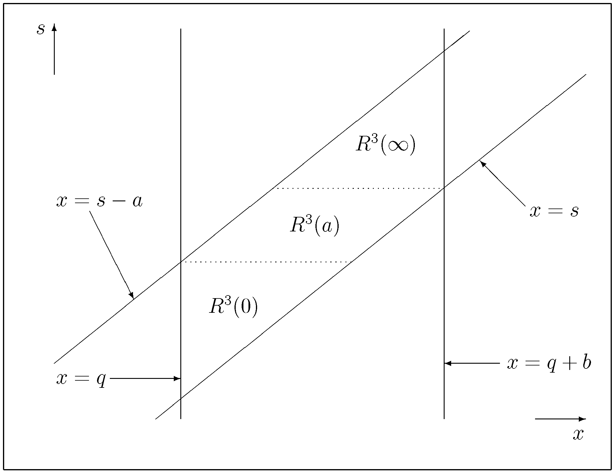
Figure 1. A computer drawing of the state space of the process ( X , S , Q ) , for some q R fixed and a < b .
Risks 07 00087 g001
Figure 2. A computer drawing of the state space of the process ( X , S , Q ) , for some q R fixed and b a .
Risks 07 00087 g002