Sound Deposit Insurance Pricing Using a Machine Learning Approach

Abstract

While the main conceptual issue related to deposit insurances is the moral hazard risk, the main technical issue is inaccurate calibration of the implied volatility. This issue can raise the risk of generating an arbitrage. In this paper, first, we discuss that by imposing the no-moral-hazard risk, the removal of arbitrage is equivalent to removing the static arbitrage. Then, we propose a simple quadratic model to parameterize implied volatility and remove the static arbitrage. The process of removing the static risk is as follows: Using a machine learning approach with a regularized cost function, we update the parameters in such a way that butterfly arbitrage is ruled out and also implementing a calibration method, we make some conditions on the parameters of each time slice to rule out calendar spread arbitrage. Therefore, eliminating the effects of both butterfly and calendar spread arbitrage make the implied volatility surface free of static arbitrage.

1. Introduction

Banks can lend or invest most of their money deposits. However, if bank’s borrowers default, the bank’s creditors, particularly depositors, risk loss. In order to protect depositors from this risk, policy makers have promoted deposit insurance schemes that are majorly issued by government run institutions. In the global scale, International Association of Deposit Insurers (IADI) was formed in 2002 “to enhance the effectiveness of deposit insurance systems by promoting guidance and international cooperation”. Even though experiences from bank runs during the 1929 Great Depression led to the introduction of the first deposit insurances in the US, they have been identified as one of the contributors to the 2008 financial crisis. The major issue due to these type of insurances is that they encourage the risk of moral hazard. While this problem has been studied to some extent in the literature (see Assa (2015) and Assa and Okhrati (2018)), there is another issue relevant to the incorrect contract design and miss-pricing which needs further attention. More precisely, in addition to the moral hazard risk, arbitrage also needs to be removed in designing a sound deposit insurance. In this paper, we first show that the removal of the arbitrage for the policies with no risk of moral hazard is tantamount to the removal of static arbitrage. This fact lead us to naturally use machine learning methods to improve the precision of estimation for implied volatility.

As it is discussed in Assa and Okhrati (2018), in a very general framework a sound deposit insurance that rules out the risk of moral hazard is a two layer policy. A two layer policy can be considered as the subtract of two European options. This helps us to use the financial engineering formalism on derivative pricing in our setting. There are some existing models for predicting the price of an option, most of which spin around the Black-Scholes model. The Black-Scholes formula is one of the most famous and frequently used methods of option pricing. However, it is derived under some constraining assumptions including variability due to the randomness of the underlying Brownian motion, no transaction costs, and fixed volatility and interest rate (Black and Scholes (1973)). In the Black-Scholes formula, all parameters are given in the market except the the stock price volatility. However, this parameter can be estimated by the past stock price data; it usually gives different Black-Scholes option prices than the market option prices because the assumption of fixed volatility does not hold in real markets. To overcome this drawback, option traders use implied volatility to adapt the market prices for options with the Black-Sholes formula. In fact, they consider an option price in terms of the Black-Sholes implied volatility.

Volatility is a measure of the variability of returns for a given security and it can be measured by the standard deviation of returns for a particular period of time usually for one year. However, implied volatility is the estimated volatility of a security’s price and it can be obtained by options trading prices based on the Black-Scholes framework. While historical volatility has only some information about underlying price fluctuation for a period of time in the past, implied volatility contains more information about option price future behavior.

The market volatility can be considered as a proxy of the bank portfolio riskiness, as proved in Zhang (2015). Volatility modeling proven to be a challenging task and there are only a few popular models for stochastic implied volatility. For instance, one can consider the stochastic alpha, beta, rho (SABR) parameterization Avellaneda (2005), Vana-Volga (VV) model Castagno (2007), a parametric model of implied volatility Zhao (2013) and Stochastic Volatility Inspired (SVI) of Gatheral (2014). Furthermore, some other studies like Malliaris (1996), Cont (2002), Alentorn (2004) and Roux (2007) tried to parameterize implied volatility using neural network, regression and other machine learning tools. However, none of these models could eliminate arbitrage opportunity.

In this study, a machine learning approach is proposed to model implied volatility and also to remove static arbitrage. Since the price of a European call option depends on the price movement of the underlying asset, we implement a quadratic machine learning approach to parametrize total implied variance for the European Black-Scholes call options with less than one year to maturity. That, how much the model is qualified to fit the implied volatility data, is verified both theoretically and empirically. We also use a regularized cost function for each volatility slice to rule out both underfitting and overfitting Hastie (2002). The main observation of this study is to explore how a regularized cost function can help eliminate static arbitrage, whereas this idea has not been successfully studied in the literature.

This paper is organized as follows: In Section 2, first we design a risk management framework, then provide some basic materials of implied volatility, static arbitrage and machine learning which are necessary for the rest of the paper. We propose a quadratic model for implied volatility and then some necessary conditions are provided on the parameters of the model to get rid of static arbitrage in Section 3. In Section 4, we implement a numerical example to illustrate the validity of the proposed model. Eventually, the paper is finished by a suggestion for future possible works in Section 5.

2. Sound Deposit Insurance

In Assa and Okhrati (2018), a deposit insurance where the risk of moral hazard is ruled out is discussed. In their paper they have shown a sound insurance contract in many cases, including when using VaR and CVaR to model the risk aversion behavior of the investors, has a two layer structure. As we want to address another caveat, that is to rule out the arbitrage, in a similar setting we use their framework. Adopting notations in Assa and Okhrati (2018), let $(\Omega ,\Im ,F={\left({\Im }_t\right)}_{0\le t\le T},\mathbb{P})$ be a completed probability space, where $\Omega$ is the set of all scenarios, $\mathbb{P}$ is the physical probability measure and ${\left({\Im }_t\right)}_{0\le t\le T}$ is a filtration with usual conditions and $\Im ={\Im }_T$ is a $\sigma$-field of measurable subsets of $\Omega$. Furthermore, $\mathbb{E}$ denotes the mathematical expectation with respect to $\mathbb{P}$. Policies are issued at $t=0$, and liabilities are settled at $t=T$. Random variables represent losses for different scenarios at time T. The cumulative distribution function associated with a random variable X is denoted by $F_X$. The market risk free interest rate is a non-negative number $r\ge 0$. Let us consider a bank with an initial capital1 $exp\left(-rT\right)b$, and a non-negative loss variable associated with the deposit insurance denoted by $\mathcal{L}\ge 0$. The bank wants to hedge its global position by transferring part of its losses to another party (usually an insurance company). The insurance policy is denoted by a non-negative random variable I and it has to satisfy $0\le I\le \mathcal{L}$. The price of the policy is given by a premium function $\pi :\mathcal{D}\to \mathbb{R}$ at time 0, where $\mathcal{D}$ is the domain of $\pi$. Therefore, the bank’s position is composed of four parts:

• The initial capital at time 0 i.e., $exp\left(-rT\right)b$;
• The global loss, $\mathcal{L}$;
• The insurance policy, $-I$;
• The premium payed for the insurance policies, at time T, $exp\left(rT\right)\pi \left(I\right)$.

Therefore, the total loss is

$$\mathrm{Total}\mathrm{loss}=exp\left(rT\right)\pi \left(I\right)+\mathcal{L}-b-I.$$

The bank wants its global position to be solvent. We use a risk measure to measure the solvency; particularly in this paper we consider Value at Risk (VaR) or Conditional Value at Risk (CVaR) recommended in the Basel II accord for the banking system (also in the Solvency II for the insurance industry). In this paper, $\varrho$ denotes the risk measure recommended by regulator. The bank is solvent if its capital b is adequate for the solvency i.e., $\varrho \left(exp\left(rT\right)\pi \left(I\right)+\mathcal{L}-b-I\right)\le 0$. Then, an optimal decision for the bank is to buy the cheapest insurance contract i.e.,

$$\left\{\begin{array}{c}min\pi \left(I\right)\hfill \\ \varrho (exp\left(rT\right)\pi \left(I\right)+\mathcal{L}-b-I)\le 0\hfill \\ 0\le I\le \mathcal{L}\hfill \end{array}\right.$$

(1)

Now, we move one step forward to use a more specific model for the bank’s asset. We use an approach similar to Merton (1997), by considering that the bank’s asset follows a geometric Brownian motion. This choice is very crucial, since one can use the risk neutral valuation in order to find the “market (consistent) value” of an insurance contract which is a necessary practice by Solvency II. Denoting the underlying by $S_t$, we assume it follows the following stochastic differential equation:

$$\left\{\begin{array}{c}d{S}_t=\mu S_{t}dt+\sigma S_{t}d{W}_t\hfill \\ S_0>0\hfill \end{array}\right.$$

Here $W_t$, $\mu$ and $\sigma$ are respectively a standard Wiener process, drift, and volatility (constant numbers). It is also known that:

$$S_t=S_{0}exp\left(\left(\mu -\frac{{\sigma }^2}{2}\right)t+\sigma W_t\right)$$

We assume that the bank’s loss is a non-negative and non-increasing function of its assets value. In mathematical terms, $\mathcal{L}=L\left(S_T\right)$, where $L:\mathbb{R}\to {\mathbb{R}}_{+}\cup \left\{0\right\}$ is a non-increasing function:

$$L\left(x\right)=\left\{\begin{array}{cc}exp\left(rT\right)S_0-x\hfill & \mathrm{if}x\le exp\left(rT\right)S_0\hfill \\ 0\hfill & \mathrm{if}x>exp\left(rT\right)S_0\hfill \end{array}\right.$$

(2)

It is clear that L is equal to ${\left(exp\left(rT\right)S_0-x\right)}_{+}$.

In Assa and Okhrati (2018) it is assumed that there is no risk of moral hazard, meaning that both bank and insurance feel risk of an adverse event. For that, Assa and Okhrati (2018) assume that both the bank and insurance loss variables are non-decreasing functions of the global loss variable. This assumption rules out the risk of moral hazard, as both sides have to feel any increase in the global loss (see for example Heimer (1989) and Bernard and Tian (2009)) Therefore, we assume that $I=f\left(\mathcal{L}\right)$ where both f and $\mathrm{id}-f$ are non-negative and non-decreasing functions (here $\mathrm{id}$ denotes the identity function).

Using the no-moral-hazard assumption, Assa and Okhrati (2018) have managed to find the sound deposit insurances where the risk of insolvency is measured by a distortion risk measure. However, in this paper we only restrain ourselves to the one mentioned by regulator (and also the most popular ones), VaR and CVaR:

$${\mathrm{VaR}}_{\alpha }\left(X\right)=inf\left\{x\in \mathbb{R}|P\left(X>x\right)\le 1-\alpha \right\},\alpha \in [0,1],$$

and

$${\mathrm{CVaR}}_{\alpha }\left(X\right)=\frac{1}{1-\alpha }{\int }_{\alpha }^1{\mathrm{VaR}}_t\left(X\right)dt.$$

(3)

For these particular risk measures, Assa and Okhrati (2018) have shown that the contract has a two-layer structure. By combining Corollary 1, Theorem 3 and Theorem 4 in Assa and Okhrati (2018) we get the following theorem:

Theorem 1.

If $\varrho ={\mathrm{VaR}}_{\alpha }$ or $\varrho ={\mathrm{CVaR}}_{\alpha }$, and $\mu -r\ge 0$ hold, then the optimal deposit insurance is a two layer policy on loss $\mathcal{L}$ i.e.,

$$I=f\left(\mathcal{L}\right),$$

where f is defined as

$$f\left(x\right)=\left\{\begin{array}{cc}0\hfill & \mathit{if}x\le l\hfill \\ x-l\hfill & \mathit{if}l\le x\le u\hfill \\ u-l\hfill & \mathit{if}u\le x\hfill \end{array}\right.,$$

(4)

for upper and lower retention levels u and l, respectively.

Now it is important to observe that such a contract can be written as the difference of two call option policies. To see this we have to take the following steps:

$$f\circ L\left(x\right)=\left\{\begin{array}{cc}0\hfill & \mathrm{if}L\left(x\right)\le l\hfill \\ L\left(x\right)-l\hfill & \mathrm{if}l\le L\left(x\right)\le u\hfill \\ u-l\hfill & \mathrm{if}u\le L\left(x\right)\hfill \end{array}\right..$$

First, observe that if $exp\left(rT\right)\le l$ then $L\left(x\right)={\left(exp\left(rT\right)S_0-x\right)}_{+}\le l$ always holds and as a result $I=0$. Otherwise, if $exp\left(rT\right)>l$, then $L\left(x\right)={\left(exp\left(rT\right)S_0-x\right)}_{+}\le l$ is equivalent to $exp\left(rT\right)S_0-l\le x$. On the other hand, $u\le \mathcal{L}={\left(exp\left(rT\right)S_0-x\right)}_{+}$ is always equivalent to $x\le exp\left(rT\right)S_0-u$. So we have the following policies:

• If $exp\left(rT\right)\le l$ then $I=0$
• If $exp\left(rT\right)>l$

  $$f\circ L\left(x\right)=\left\{\begin{array}{cc}0\hfill & \mathrm{if}exp\left(rT\right)S_0-l\le x\hfill \\ exp\left(rT\right)S_0-x-l\hfill & \mathrm{if}exp\left(rT\right)S_0-u\le x\le exp\left(rT\right)S_0-l\hfill \\ u-l\hfill & \mathrm{if}x\le exp\left(rT\right)S_0-u\hfill \end{array}\right..$$

  or

  $$f\circ L\left(x\right)={\left(x-exp\left(rT\right)S_0+l\right)}_{+}-{\left(x-exp\left(rT\right)S_0+u\right)}_{+}+u-l.$$

This indicates that I can be written as the difference of two call options

$$I={\left(S_T-exp\left(-rT\right)S_0+l\right)}_{+}-{\left(S_T-exp\left(-rT\right)S_0+u\right)}_{+}+u-l.$$

(5)

Now, we want to introduce the risk premium. An important implication of what we have done above is that all insurance contracts are in the form of a contingent claim i.e., for $f\in \mathbb{C}$, $f\left(\mathcal{L}\right)=f\left(L\left(S_T\right)\right)=\left(f\circ L\right)\left(S_T\right)$. To find the market value of a contingent claim we use the no-arbitrage valuation, so we have:

$$\pi \left(I\right)=exp\left(-rT\right)\mathbb{E}\left(\frac{d\mathbb{Q}}{d\mathbb{P}}I\right)=exp\left(-rT\right){\mathbb{E}}^{*}\left(I\right),$$

where $\frac{d\mathbb{Q}}{d\mathbb{P}}$ is the Radon-Nikodym derivative of the risk neutral probability measure $\mathbb{Q}$ with respect to $\mathbb{P}$ and $E^{*}$ is the expectation with respect to this measure. However, as we have seen in (5), this contract can be written as the difference of two call options plus a constant value. So we can then use the following valuation of the contract in our setup

$$\begin{array}{c}\pi \left(I\right)=e^{-rT}{E}^{*}\left(I\right)\hfill \\ =C_{BS}\left(S_0,exp\left(rT\right)S_0-l,T,\sigma ,r\right)-C_{BS}\left(S_0,exp\left(rT\right)S_0-u,T,\sigma ,r\right)\\ \hfill +exp\left(-rT\right)\left(u-l\right),\end{array}$$

(6)

where in general $C_{BS}\left(S_0,K,\tau ,\sigma ,r\right)$ denotes the value of a call option with maturity $\tau$, strike price K, volatility $\sigma$, interest rate r and initial underlying value $S_0$, in a Black-Scholes model. So we have the following corollary:

Corollary 1.

If $\varrho ={\mathrm{VaR}}_{\alpha }$ or $\varrho ={\mathrm{CVaR}}_{\alpha }$, and $\mu -r\ge 0$ hold, then the optimal deposit insurance is the difference of two call options plus a constant value. As a result, for a no-arbitrage valuation, the no-arbitrage assumption needs only to hold for the call options.

2.1. Black-Scholes Model

The price of a European style call option Black and Scholes (1973) is calculated as follows:

$$\begin{array}{cc}\hfill C_{BS}\left(S_0,K,\tau ,\sigma ,r\right)& =exp\left(-r\tau \right)E{\left(S_T-K\right)}_{+}\hfill \\ & =S_{0}N\left(d_1\right)-exp\left(-r\tau \right)KN\left(d_2\right)\hfill \end{array}$$

(7)

$$d_1=\frac{ln\left(\frac{S_0}{K}\right)+\left(r+\frac{{\sigma }^2}{2}\right)\tau }{\sigma \sqrt{\tau }},d_2=d_1-\sigma \sqrt{\tau }$$

where $S_0$ denotes the risky asset price at time 0, K is the exercise price, $\tau$ is the time to expiration, $\sigma$ is the standard deviation of the security’s return, N is the distribution function for the standard normal distribution, and r is the rate of interest.

2.2. Implied Volatility

The implied volatility of a risky asset S is the unique value of ${\sigma }_{imp}$ that solves the following equation

$$C=C_{BS}\left(\tau ,K,\tau {\sigma }_{imp}^2,S,r,t\right)$$

(8)

where C is the market price for the call option written at time t with strike price K and T is the expiration time.

Another version of implied volatility is calculated by the underlying price process being replaced by the forward price in the Black-Scholes model. This version of implied volatility has some nice properties that facilitate application of mathematical techniques. The Black formula is as follows:

$$C_B\left(\tau ,K,\tau {\sigma }_{imp}^2,S,r,t\right)=F_{\left[t,t+\tau \right]}N\left(d_1\right)-KN\left(d_2\right)$$

(9)

$$d_1=\frac{log\left(\frac{F_{\left[t,t+\tau \right]}}{k}\right)+\frac{1}{2}\tau {\sigma }_{imp}^2}{\sqrt{\tau {\sigma }_{imp}^2}},d_2=\frac{log\left(\frac{F_{\left[t,t+\tau \right]}}{k}\right)-\frac{1}{2}\tau {\sigma }_{imp}^2}{\sqrt{\tau {\sigma }_{imp}^2}}$$

where $F_{\left[t,t+\tau \right]}=exp\left(-r\tau \right)S_t$ is the forward price.

2.3. Static Arbitrage

Now, we provide mathematical definition Roper (2009) of static arbitrage and then present an equivalent definition which connects it to the two other types of arbitrage called calendar spread and butterfly.

Definition 1.

A surface of call option C is said to be free of static arbitrage if there exists a non-negative martingale X on $(\Omega ,\Im ,\mathcal{F}={\left({\Im }_t\right)}_{t\ge 0},\mathbb{P})$ which the call price formula can be reached by

$$C(K,\tau )=E\left({\left(X_{\tau }-k\right)}_{+}\right),\forall (k,\tau )\in [0,\infty )\times [0,\infty )$$

(10)

In other words, there exists a non-negative martingale which is associated with the security price process in distribution, in fact both the security price and the equivalent martingale follow the same probabilistic rules. The next two theorems by Kellerer (1972) provide some conditions on call surface and some equivalent conditions on volatility surfaces to make them free of static arbitrage.

Theorem 2.

A call option surface written on underlying S, with expiration time T

$$\begin{array}{c}C:\left(0,\infty \right)\times R\to \left(0,\infty \right)\hfill \\ \left(\tau ,k\right)\to E\left({\left(S_T-k\right)}_{+}\right)\hfill \end{array}$$

is said to be free from static arbitrage if the following conditions are satisfied:

1.

${\partial }_{\tau }C>0$

2.

$\underset{k\to \infty }{lim}C(\tau ,k)=0$

3.

$\underset{k\to -\infty }{lim}C(\tau ,k)+k=a,a\in R$

4.

$C(\tau ,k)\mathit{is}\mathit{convex}\mathit{in}k$

5.

$C(\tau ,k)\ge 0$

Theorem 3.

On the surface of total implied variance $w_{imp}=\tau {\sigma }_{imp}^2$ where

$$\begin{array}{c}{w}_{imp}:\left(0,\infty \right)\times R\to \left(0,\infty \right),\hfill \\ \left(\tau ,K\right)\to w_{imp}\left(\tau ,K\right),\hfill \end{array}$$

The conditions in Theorem 2 are derived by the following arguments

1.

${\partial }_{\tau }{w}_{imp}>0;$

2.

$\underset{k\to \infty }{lim}{d}_1\left(k\right)=-\infty ;$

3.

$\tau {\sigma }_{imp}\ge 0;$

4.

${\left(1-\frac{x}{2w_{imp}}{\partial }_x\left(w_{imp}\right)\right)}^2-\frac{1}{4}\left(\frac{1}{w_{imp}}-\frac{1}{4}\right){\left({\partial }_x\left(w_{imp}\right)\right)}^2+\frac{1}{2}{\partial }_{xx}\left(w_{imp}\right)\ge 0.$

The first condition in Theorem 3 which implies the first one in Theorem 2 means that total implied variance is increasing with respect to time to maturity. Moreover, if this condition holds, there is no calendar spread arbitrage Fengler (2009), otherwise the opportunity of calendar spread arbitrage emerges in the market, so one can do a risk-free trading strategy at a given moment. As a matter of fact, the existence of calendar spread arbitrage addresses a trader to buy a nearby option and sell the farther in the case of the large time spread between the two options and sell the nearby and buy the farther if the spread is narrow Carr and Madan (2005). Conditions 2 and 3 in Theorem 3 imply condition 2 of Theorem 2 which reveals that the price of an option for large exercise prices, tends to zero. The third argument in Theorem 2 is derived by conditions 2, 3 and 4 in Theorem 3. Finally, the inequality 4, known as Durrleman’s condition Durrleman (2003), is a part of the second derivative of call surface with respect to strike price.

Conditions 2 and 4 in Theorem 3 provide a volatility surface free of butterfly arbitrage. For example, let $C_1$ and $C_2$ are two call options with expiration time T and exercise prices $K_i$ that $K_1<K_2$, and suppose an option with the same maturity time T and the strike price K, where $K_1<K<K_2$, exists in the market. If the call surface is non-convex with respect to exercise price, there is an opportunity to sell two options at the middle strike price K and buy one at the strike price $K_1$ and one at the strike price $K_2$ and by this strategy a trader can gain a risk-free profit. So, condition 4 of Theorem 3 assigns a non-negative value for the second derivative of a call surface to get rid of butterfly arbitrage.

Now it is time to provide another definition for a volatility call surface Gatheral (2011) to make it free of static arbitrage based on materials related to both types of arbitrage, calendar spread and butterfly.

Definition 2.

There is no static arbitrage on a volatility surface if and only if

1.

It is free of calendar spread arbitrage;

2.

The volatility slice is free of butterfly arbitrage for any fixed time to maturity.

Particularly, no butterfly arbitrage is equivalent to the existence of a positive probability density Breeden and Breeden and Litzenberger (1978), and no calendar spread arbitrage implies that the option price is increasing with respect to time to expiration.

2.4. Parameterization of the Implied Volatility

For a fixed time to expiration, the SVI model Gatheral (2004) is given by

$$w_{imp}^{SVI}\left(x\right)=a+b(\rho \left(x-m\right)+\sqrt{{\left(x-m\right)}^2+{\sigma }^2})$$

(11)

$$a\in \mathbb{R},b\ge 0,\left|\rho \right|<1,m\in \mathbb{R},\sigma >0,x=log\frac{K}{F_{[t,t+\tau ]}}$$

in this parametrization, x is moneyness, $w_{imp}^{SVI}\left(x\right)=\tau {\sigma }_{imp}^2$ is total implied variance and $\left\{a,b,\sigma ,\rho ,m\right\}$ is the set of parameters that are supposed to be estimated. The behavior of volatility smile is highly affected by variations in these five parameters; moreover, the reason to use total implied variance instead of implied volatility is that in Equation (9) the volatility parameter $\sigma$ is always accompanied with a $\sqrt{\tau }$ Zhu (2013).

2.5. Machine Learning Approach

Machine learning is a branch of artificial intelligence (AI) that has many applications used to model the behavior of natural phenomena and predict their future outcomes. The basic intuition behind this methodology is that there is a training set that consists of empirical data $(x^{\left(1\right)},y^{\left(1\right)}),(x^{\left(2\right)},y^{\left(2\right)}),\dots ,(x^{\left(m\right)},y^{\left(m\right)})$, where m is the number of training examples; moreover, a learning algorithm (learning hypothesis) fits the data to determine how to learn from the training set and how well the result can be generalized to the unseen data. The vector of parameters $\theta$ is reached by the following strategy:

$$\widehat{\theta }=arg\underset{\theta }{min}J\left(\theta \right)=arg\underset{\theta }{min}\frac{1}{2m}\sum _{i=1}^{m}V\left(h_{\theta }\left(x^{\left(i\right)}\right),y^{\left(i\right)}\right)$$

(12)

V is the cost of predicting $y^{\left(i\right)}$ based on hypothesis $h_{\theta }\left(x^{\left(i\right)}\right)$ for the i-th training example. The cost V for the i-th training example is a function of the difference between the target value $y^{\left(i\right)}$ and the estimated values $h_{\theta }\left(x^{\left(i\right)}\right)$. Usually this function is considered to be L-1 norm or L-2 norm loss function that the L-1 norm is absolute difference and the L-2 norm is the square difference. A learning hypothesis is a predetermined function, usually chosen by experts, that is considered to fit the data to describe its behavior inside and outside the training set.

However, sometimes choosing an adequate learning algorithm which best describes the trend of data outside the training set is the area of difficulty and a wrong learning algorithm takes a lot of time investigating without coming up to a real conclusion. So, we should know what is the best promising avenue to spend time pursuing. If our selected hypothesis does an excellent job predicting y from x for observations in the training set but not for those outside the training set, we face overfitting, on the other hand, if the hypothesis does not do well, predicting y in both the training set and outside the training set, we encounter underfitting. Most of the time the algorithm is faced with overfitting since a learning algorithm usually does a good job for data that builds the model and the problem is how well it fits to the unseen data. Conquering these obstacles, we add a regularization term to the cost function and estimate parameters as follows:

$$\widehat{\theta }=arg\underset{\theta }{min}\frac{1}{2m}\left(V\left(h_{\theta }\left(x^{\left(i\right)}\right),y^{\left(i\right)}\right)+\lambda R\left(h_{\theta }\left(x^{\left(i\right)}\right)\right)\right)$$

(13)

The penalty term is used when there is model complexity, in other words, as long as the algorithm encounters underfitting or overfitting the penalty term keeps the parameters small to preclude these types of complexity. To give a break down explanation of regularization, the parameter $\lambda$ is called the regularization parameter assigned to control the trade-off between underfitting and overfitting. $\mathit{R}$ is the regularization function which provides a penalty for the hypothesis complexity to impose some certain restrictions on parameters space. Furthermore, the regularization function improves the hypothesis to generalize well to the data beyond the training set Nilsson (2005).

There are some methods to debug a learning algorithm to rule out underfitting and overfitting. To fix overfitting, we can get more training examples try smaller sets of features and try increasing $\lambda$; moreover, to rule out underfitting, some adjustments like getting additional features, adding polynomial features, and trying to decrease $\lambda$ are helpful according to Hastie (2002).

3. The Quadratic Parametrization

Different types of quadratic models have been proposed for implied volatility parameterization in recent years, but none of them are qualified enough to be free of static arbitrage. For instance, Avellaneda (2005) proposed a quadratic model to parameterize implied volatility, however, as mentioned in Roper (2010), this model does not guarantee the Durrleman’s function to be everywhere non-negative around ATM, so the absence of butterfly arbitrage is not satisfied. There are some other types of quadratic models, like Roux (2007), but there is no condition on the parameters to remove static arbitrage, hence it is seemingly impossible to be encountered with this inadequacy in the area of quadratic parametrization of implied volatility. Now, we introduce our proposed quadratic model to parameterize implied volatility for call options with less than one year time to expiration, then provide some special conditions on the model parameters, we preclude static arbitrage.

3.1. The Raw Quadratic Model

The quadratic parameterization of total implied variance with respect to moneyness $\mathit{x}$ is given by:

$$w_{imp}^{Q^2}(x,\eta )={\theta }_0+{\theta }_{1}x+{\theta }_2{x}^2$$

(14)

where ${\theta }_0>0,{\theta }_1\in \mathbb{R}$. The condition of ${\theta }_2>0$ along with the condition of ${\theta }_1^2-4{\theta }_0{\theta }_2<0$ make the function $x\to w_{imp}^{Q^2}\left(x,\eta \right)$ positive and strictly convex for all $x\in \mathbb{R}$.

3.2. Elimination of Static Arbitrage

In this section, we present some conditions on the parameters of the quadratic model (14) to make it free of static arbitrage. However, since (14) is a model with fixed time to maturity, we introduce an equivalent parameterization for implied variance with respect to ATM variance, ATM volatility skew and the lower bound of variance. Then, we make some conditions on the parameters of the equivalent model to guarantee the absence of calendar spread arbitrage. These parameters are more familiar for market traders than the raw parameters in (14) since they reveal some characteristics of market data which are known for investors. The idea begins with the following definition.

Definition 3.

For a fixed time to maturity and a parameter set $\chi =\left\{v_{\tau },{\psi }_{\tau },{\mu }_{\tau }\right\}$, the equivalent quadratic parameterization of implied variance is

$${\sigma }_{imp}^2=v_{\tau }+\left(2\sqrt{v_{\tau }}{\psi }_{\tau }\right)x+\left(\frac{v_{\tau }{\psi }^2}{v_{\tau }-{\mu }_{\tau }}\right)x^2$$

(15)

$$v_{\tau }>0,{\psi }_{\tau }\in \mathbb{R},{\mu }_{\tau }>0,$$

where $v_{\tau }$ is ATM variance, ${\psi }_{\tau }$ is ATM volatility skew, and ${\mu }_{\tau }$ is the minimum level of variance. Therefore, this is a calibration to three given quantities which are more understandable for market traders than the raw parameters. For a fixed time to maturity, the following relations hold between the raw parameters and the equivalent quadratic parameters:

$$v_{\tau }=\frac{{\theta }_0}{\tau },{\psi }_{\tau }=\frac{1}{\sqrt{\tau }}\frac{{\theta }_1}{2\sqrt{{\theta }_0}},{\mu }_{\tau }=\frac{1}{\tau }\left({\theta }_0-\frac{\theta {}_1^2}{4{\theta }_2}\right)$$

Proposition 1.

The equivalent parameterization of implied variance is not affected by calendar spread arbitrage if the following arguments are held

1.

${\psi }_{\tau }\left({\partial }_{\tau }{\psi }_{\tau }\right)>0$

2.

${\partial }_{\tau }\left[ln\left(\frac{v_{\tau }}{v_{\tau }-{\mu }_{\tau }}\right)\right]>\frac{\left(v_{\tau }-{\mu }_{\tau }\right)}{4v_{\tau }^3}$

3.

${\partial }_{\tau }\left[ln{\psi }_{\tau }\right]<\frac{2v_{\tau }}{v_{\tau }-{\mu }_{\tau }}-\frac{1}{v_{\tau }}$

Proof. 

We are supposed to show that the following expression, which is the first derivative of the surface with respect to time to maturity, always takes positive values

$$\begin{array}{cc}\hfill {\partial }_{\tau }{\sigma }_{imp}^2=& {\partial }_{\tau }{v}_{\tau }+2\left\{\frac{{\psi }_{\tau }}{2\sqrt{v_{\tau }}}+\sqrt{v_{\tau }}\left({\partial }_{\tau }{\psi }_{\tau }\right)\right\}x\hfill \\ \hfill +& \left\{\frac{\left\{2{\psi }_{\tau }\left({\partial }_{\tau }{\psi }_{\tau }\right)v_{\tau }+{\psi }_{\tau }^2\left({\partial }_{\tau }{v}_{\tau }\right)\right\}(v_{\tau }-{\mu }_{\tau })-\left\{v_{\tau }{\psi }_{\tau }^2{\partial }_{\tau }(v_{\tau }-{\mu }_{\tau })\right\}}{{(v_{\tau }-{\mu }_{\tau })}^2}\right\}{x}^2.\hfill \end{array}$$

Since this is a quadratic function of x, we just need to show that the coefficient of the highest degree is positive and the discriminant is negative. So, doing some rearrangement of the numerator of the coefficient in the highest degree, we should proof the following inequality:

$$\left\{2{\psi }_{\tau }\left({\partial }_{\tau }{\psi }_{\tau }\right)v_{\tau }\right\}(v_{\tau }-{\mu }_{\tau })+{\psi }_{\tau }^2\left\{\left({\partial }_{\tau }{v}_{\tau }\right)(v_{\tau }-{\mu }_{\tau })-v_{\tau }{\partial }_{\tau }(v_{\tau }-{\mu }_{\tau })\right\}>0$$

The above inequality is satisfied based on conditions 1 and 2 since $v_{\tau }$ and $(v_{\tau }-{\mu }_{\tau })$ are positive due to the initial conditions on raw quadratic parameters of Section 3.1. Another step to make the quadratic function everywhere non-negative is to make the discriminant everywhere negative since a strictly positive quadratic function should not cross the x axis. Therefore, by some simple rewriting of the discriminant we come up with the following inequality:

$$a=\frac{v_{\tau }{\psi }_{\tau }^2}{v_{\tau }-{\mu }_{\tau }},b=2\sqrt{v_{\tau }}{\psi }_{\tau },c=v_{\tau }$$

$$\begin{array}{cc}\hfill 4ac-b^2=& 4{\psi }_{\tau }^2{v}_{\tau }^2\left\{\left\{\left({\partial }_{\tau }{v}_{\tau }\right)(v_{\tau }-{\mu }_{\tau })-v_{\tau }{\partial }_{\tau }(v_{\tau }-{\mu }_{\tau })\right\}-\frac{{(v_{\tau }-{\mu }_{\tau })}^2}{4v_{\tau }^2}\right\}\hfill \\ \hfill +& 4v_{\tau }{\psi }_{\tau }\left({\partial }_{\tau }{\psi }_{\tau }\right)(v_{\tau }-{\mu }_{\tau })\left\{2v_{\tau }^2-\left\{v_{\tau }\frac{\left({\partial }_{\tau }{\psi }_{\tau }\right)}{{\psi }_{\tau }}+1\right\}(v_{\tau }-{\mu }_{\tau })\right\}>0.\hfill \end{array}$$

So, we are supposed to make the above function strictly positive by providing some conditions on the three introduced parameters. The first part of the function above is positive due to the condition 2, and the second part is non-negative based on conditions 1 and 3. So, our convex quadratic model never crosses the x axis. Therefore, the proof is complete. ☐

Note that, in the previous proposition we provided some conditions on the parameters which are familiar for market traders and each of them is a function of time to maturity. So, to implement this strategy to market data all these parameters should be available in terms of expiry time. In the next proposition, we provide some conditions on the raw parameters to rule out static arbitrage. We will discuss ways and means of implementing this strategy to market data in Section 4.

Proposition 2.

The quadratic surface 14 is not influenced by calendar spread arbitrage if for any two times to maturity ${\tau }_1<{\tau }_2$ corresponding to $w(.,{\tau }_1)$ and $w(.,{\tau }_2)$ by the parameters sets ${\eta }_1=\{{\theta }_{01},{\theta }_{11},{\theta }_{21}\}$ and ${\eta }_2=\{{\theta }_{02},{\theta }_{12},{\theta }_{22}\}$ the following conditions satisfy:

1.

${\theta }_{22}-{\theta }_{21}>0;$

2.

${\theta }_{22}{\theta }_{01}+{\theta }_{21}{\theta }_{02}<\frac{{\theta }_{12}{\theta }_{11}}{2}.$

Proof. 

To show that the two volatility slices never cross each other we should prove that the following quadratic function takes positive values everywhere. Hence, it should be a convex function with no real root

$$w(.,{\tau }_2)-w(.,{\tau }_1)=({\theta }_{22}-{\theta }_{21})x^2+({\theta }_{12}-{\theta }_{11})x+({\theta }_{02}-{\theta }_{01}).$$

(16)

Condition 1 guarantees the quadratic Function (16) to be convex. In addition, we need to show that it does not have a real root, so the discriminant should take a negative value

$$\begin{array}{cc}\hfill \Delta =& {({\theta }_{12}-{\theta }_{11})}^2-4({\theta }_{22}-{\theta }_{21})({\theta }_{02}-{\theta }_{01})\hfill \\ \hfill =& ({\theta }_{12}^2-4{\theta }_{22}{\theta }_{02})+({\theta }_{11}^2-4{\theta }_{21}{\theta }_{01})+4({\theta }_{22}{\theta }_{01}+{\theta }_{21}{\theta }_{02})-2{\theta }_{12}{\theta }_{11}\hfill \end{array}$$

The first two terms are negative based on the initial conditions in Section 3.1, and also condition 2 makes the other two expressions negative. Therefore, $\Delta <0$ and the proof is complete. ☐

So, we use these conditions to parametrize total implied variance slice by slice. This means they play the role of optimization constraints for each fixed time to maturity to preclude calendar spread arbitrage. A common approach is a forward strategy which performs these conditions separately for the shortest time to expiration up to the longest one. Now, we set some conditions on the parameters to make a volatility slice free of butterfly arbitrage.

Proposition 3.

The quadratic volatility model in Section 3.1, for options with less than one year to maturity ($\tau <1$), is free of butterfly arbitrage if

1.

${\theta }_1^2-4{\theta }_0{\theta }_2+{\theta }_2<0;$

2.

$\frac{1}{4}<{\theta }_0<1.$

Proof. 

First of all, we show that the minimum value of the proposed model belongs to the interval $[0,1]$ since we assumed options with less than one year expiry time which makes $w_{imp}^{Q^2}$ bounded between 0 and 1. So, the inequality $0<w_{imp}^{Q^2}(-\frac{{\theta }_1}{2{\theta }_2},\eta )<1$ and equivalently the inequality $4({\theta }_0-1){\theta }_2<{\theta }_1^2<4{\theta }_0{\theta }_2$ must be held. It is easily satisfied because of conditions 2 and also the initial conditions of Section 3.1. Moreover, another intuition behind the condition ${\theta }_0<1$ is to guarantee the model to be less than one in case of ATM. Now, we do some rearrangement to make the Durrleman’s function take positive values everywhere.

$$\begin{array}{cc}\hfill g\left(x\right)=& {\left(1-\frac{x}{2w}{\partial }_x\left(w\right)\right)}^2-\frac{1}{4}\left(\frac{1}{w}-\frac{1}{4}\right){\left({\partial }_x\left(w\right)\right)}^2+\frac{1}{2}{\partial }_{xx}\left(w\right)\hfill \\ \hfill =& {\left(1-\frac{x({\theta }_1+2{\theta }_{2}x)}{2({\theta }_0+{\theta }_{1}x+{\theta }_2{x}^2)}\right)}^2+\left(-\frac{{({\theta }_1+2{\theta }_{2}x)}^2}{4({\theta }_0+{\theta }_{1}x+{\theta }_2{x}^2)}-\frac{{({\theta }_1+2{\theta }_{2}x)}^2}{16}+{\theta }_2\right)\hfill \\ \hfill =& f\left(x\right)+h\left(x\right)\hfill \end{array}$$

For the Durrleman’s function g, we begin with the first expression as follows:

$$f\left(x\right)={\left(1-\frac{x({\theta }_1+2{\theta }_{2}x)}{2({\theta }_0+{\theta }_{1}x+{\theta }_2{x}^2)}\right)}^2=1+\frac{x^2{({\theta }_1+2{\theta }_{2}x)}^2}{4{({\theta }_0+{\theta }_{1}x+{\theta }_2{x}^2)}^2}-\frac{x{\theta }_1+2{\theta }_2{x}^2}{{\theta }_0+{\theta }_{1}x+{\theta }_2{x}^2}$$

Rearranging the third term of function f, we get the following function:

$$\begin{array}{cc}\hfill \frac{x({\theta }_1+2{\theta }_{2}x)}{{\theta }_0+{\theta }_{1}x+{\theta }_2{x}^2}=& \frac{{\theta }_{1}x+{\theta }_2{x}^2+{\theta }_2{x}^2+{\theta }_0-{\theta }_0}{{\theta }_0+{\theta }_{1}x+{\theta }_2{x}^2}=\frac{{\theta }_0+{\theta }_{1}x+{\theta }_2{x}^2+{\theta }_2{x}^2-{\theta }_0}{{\theta }_0+{\theta }_{1}x+{\theta }_2{x}^2}\hfill \\ \hfill =& 1+\frac{{\theta }_2{x}^2-{\theta }_0}{{\theta }_0+{\theta }_{1}x+{\theta }_2{x}^2}\hfill \end{array}$$

Therefore, we have

$$\begin{array}{cc}\hfill f\left(x\right)=& {\left(1-\frac{x({\theta }_1+2{\theta }_{2}x)}{2w}\right)}^2=1+\frac{x^2{({\theta }_1+2{\theta }_{2}x)}^2}{4w^2}-1-\frac{{\theta }_2{x}^2-{\theta }_0}{w}\hfill \\ \hfill =& \frac{{\theta }_1^2{x}^2+4{\theta }_1{\theta }_2{x}^3+4{\theta }_2^2{x}^4-4{\theta }_0{\theta }_2{x}^2+4{\theta }_0^2-4{\theta }_1{\theta }_2{x}^3+4{\theta }_0{\theta }_{1}x-4{\theta }_2^2{x}^4+4{\theta }_0{\theta }_2{x}^2}{4w^2}\hfill \\ \hfill =& \frac{{\theta }_1^2{x}^2+4{\theta }_0{\theta }_{1}x+4{\theta }_0^2}{4w^2}\hfill \end{array}$$

Since ${\theta }_1^2>0$ and $\Delta =0$, the numerator of f is a convex and strictly positive quadratic function which takes its minimum value at x = 0

$$f\left(\frac{-4{\theta }_0{\theta }_1}{2{\theta }_1^2}\right)=f\left(\frac{-2{\theta }_0}{{\theta }_1}\right)=4{\theta }_0^2-8{\theta }_0^2+4{\theta }_0^2=0$$

So, regardless of the value of the parameters, the convex function f takes its minimum at 0, so we are not supposed to subtract any positive value from function f because we desire to make the Durrleman’s function g everywhere positive. Now we have to work on other parts of g, working toward making some conditions on the parameters to rule out butterfly arbitrage. Based on condition 1 we have

$$\begin{array}{cc}\hfill {({\theta }_1+2{\theta }_{2}x)}^2=& {\theta }_1^2+4{\theta }_1{\theta }_{2}x+4{\theta }_2^2{x}^2\hfill \\ \hfill \le & 4{\theta }_0{\theta }_2+4{\theta }_1{\theta }_{2}x+4{\theta }_2^2{x}^2=4{\theta }_{2}w\hfill \end{array}$$

So, the following inequality is satisfied for the function h

$$\begin{array}{cc}\hfill h\left(x\right)=& -\frac{{({\theta }_1+2{\theta }_{2}x)}^2}{4w}-\frac{{({\theta }_1+2{\theta }_{2}x)}^2}{16}+{\theta }_2\hfill \\ \hfill \ge & \frac{4w{\theta }_2-{({\theta }_1+2{\theta }_2)}^2}{4w}-\frac{4{\theta }_{2}w}{16}\hfill \\ \hfill =& \frac{1}{4}\left(\frac{4{\theta }_0{\theta }_2-{\theta }_1^2}{w}-{\theta }_{2}w\right)\hfill \end{array}$$

Since we assume this parameterization for options with less than one year to expiration $(\tau <1)$, we have $w=\tau {\sigma }_{imp}^2<1$; thus, the fact that $-w\ge -\frac{1}{w}$ lets us make the function h everywhere positive

$$\begin{array}{cc}\hfill h\left(x\right)\ge & \frac{1}{4}\left(\frac{4{\theta }_0{\theta }_2-{\theta }_1^2}{w}-\frac{{\theta }_2}{w}\right)=\frac{1}{4}\left(\frac{4{\theta }_0{\theta }_2-{\theta }_1^2-{\theta }_2}{w}\right)\hfill \\ \hfill =& \frac{1}{4}\left(\frac{{\theta }_2(4{\theta }_0-1)-{\theta }_1^2}{w}\right)\ge 0.\hfill \end{array}$$

The last inequality is satisfied because of the first and second conditions we assumed for the model, so $g\left(\theta \right)\ge 0$. Note that we limit our work on options with less than one year to maturity, hence the data we use as w is between 0 and 1. Now we show that the second condition in Theorem 3 is satisfied

$$\begin{array}{cc}\hfill \underset{k\to \infty }{lim}{d}_1\le lim\underset{k\to \infty }{sup}{d}_1=& lim\underset{k\to \infty }{sup}\frac{log\left(\frac{F_{\left[t,t+\tau \right]}}{k}\right)+\frac{1}{2}\tau {\sigma }_{imp}^2}{\sqrt{\tau {\sigma }_{imp}^2}}\hfill \\ \hfill =& lim\underset{x\to -\infty }{sup}\frac{x+\frac{1}{2}({\theta }_0+{\theta }_{1}x+{\theta }_2{x}^2)}{\sqrt{{\theta }_0+{\theta }_{1}x+{\theta }_2{x}^2}}\hfill \\ \hfill =& lim\underset{u\to \infty }{sup}\frac{-u+\frac{1}{2}({\theta }_0-{\theta }_{1}u+{\theta }_2{u}^2)}{\sqrt{{\theta }_0-{\theta }_{1}u+{\theta }_2{u}^2}}\hfill \\ \hfill =& lim\underset{u\to \infty }{sup}\frac{-\sqrt{u}}{\sqrt{2}}\left(\frac{\sqrt{2u}}{\sqrt{{\theta }_0-{\theta }_{1}u+{\theta }_2{u}^2}}-\frac{\sqrt{{\theta }_0-{\theta }_{1}u+{\theta }_2{u}^2}}{\sqrt{2u}}\right)\hfill \end{array}$$

Roper (2010) proved that if the superior limit of the second term in parenthesis tends to a constant in the interval [0, 1), then the last limit above goes to minus infinity

$$lim\underset{u\to \infty }{sup}\frac{\sqrt{{\theta }_0-{\theta }_{1}u+{\theta }_2{u}^2}}{\sqrt{2u}}<lim\underset{u\to \infty }{sup}\frac{1}{\sqrt{2u}}=0\in [0,1)$$

The inequality above is satisfied because we set ${\theta }_1\in \mathbb{R}$, therefore $\underset{k\to \infty }{lim}{d}_1=-\infty$ and the proposed model is free of butterfly arbitrage. ☐

Now, due to the Propositions 1 and 3, we come up with the following conclusion that provides some conditions to rule out static arbitrage when we parametrize implied variance with respect to ATM variance, ATM volatility skew and the minimum level of variance.

Theorem 4.

The equivalent parameterization of implied variance for options with less than one year to maturity, is not faced with static arbitrage if

1.

${\psi }_{\tau }\left({\partial }_{\tau }{\psi }_{\tau }\right)>0$

2.

${\partial }_{\tau }\left[ln\left(\frac{v_{\tau }}{v_{\tau }-{\mu }_{\tau }}\right)\right]>\frac{\left(v_{\tau }-{\mu }_{\tau }\right)}{4v_{\tau }^3}$

3.

${\partial }_{\tau }\left[ln{\psi }_{\tau }\right]<\frac{2v_{\tau }}{v_{\tau }-{\mu }_{\tau }}-\frac{1}{v_{\tau }}$

4.

$0<\tau v_{\tau }<\frac{1}{4}$

5.

$\frac{v_{\tau }{\psi }_{\tau }^2}{v_{\tau }-{\mu }_{\tau }}\left(4\tau {\mu }_{\tau }-1\right)>0$

So far, we have provided some conditions that guarantee the absence of static arbitrage; thus, we have everything to fit the proposed quadratic model to implied volatility data.

4. Numerical Implementation

In this section, we provide a learning algorithm to modeling implied volatility data which is earned by S&P 500 European call options written on 15 December 2014. In other words, we consider bank asset to be S&P 500 index fund and we implement the proposed strategy to price call options written on this asset. The reason to choose S&P 500 as underlying asset is the simplicity and availability of this important data to make the numerical part move straightforward upon a well-defined path; whereas, underlying price process $S_t$, can be replaced by any type of risky asset.

The idea behind our strategy is that since the total implied variance of a security price is a smile-shaped function of log-moneyness, we fit the quadratic model 14 to the data. In other words, instead of just learning from input data x, we learn based on a mapping from x to its second degree polynomial. The training set of this investigation includes x as log-moneyness and w as total implied variance. To improve the robustness of the algorithm, training set data is randomly divided into two portions: 70% for the training set and 30% for the cross-validation set. The cost function consists of a penalty to control the trade-off between underfitting and overfitting. Finally, to illustrate the efficiency of the proposed approach, we perform it for six different times to maturity.

4.1. The Cost Function

The cost function we use to estimate the parameters of each volatility slice (for a fixed time to maturity) is a machine learning regularized cost function and the parameters are estimated by the following strategy:

$$\widehat{\theta }=arg\underset{\theta }{min}\frac{1}{2m}\left(\sum _{i=1}^m{\left(w_{\theta }^{Q^2}\left(x^{\left(i\right)}\right)-w^{\left(i\right)}\right)}^2+\lambda \sum _{j=1}^2{\theta }_j^2\right)$$

(17)

$w^{\left(i\right)}$ is the corresponding total implied variance for the i-th training example and $w_{\theta }^{Q^2}\left(x^{\left(i\right)}\right)$ is the quadratic model proposed in Section 3.1 and in this case, it plays the role of learning hypothesis. The cost function is a L-2 norm loss function plus a penalty term. L-2 function is chosen because it is the most common cost function; furthermore, it has one stable solution whereas the L-1 loss function has unstable and possibly multiple solutions. Since the goal is to estimate the parameters of a quadratic model, a L-2 regularization term is reasonable, and it encourages parameter values toward zero, but not exactly zero; moreover, the distribution of parameters is approximately a zero mean normal distribution. In case of model complexity (High test error), the penalty term keeps the parameters small to make the hypothesis relatively simple to avoid overfitting. $\lambda$ is the regularization parameter that controls the trade-off between underfitting and overfitting.

When we choose a lambda value, the goal is to provide the right balance between simplicity and training-data fit. If lambda is too high, the model will be simple, but we may face the risk of underfitting and the model will not learn enough from the training set to make useful predictions. On the other hand, if lambda is too low, there is more model complexity, and we encounter the risk of overfitting; in addition, the model will learn too much from the training set and will not be able to generalize to unseen data. The ideal value of lambda provides a model that generalizes well to the data outside the training set, but it depends on data and we need to do some tuning. Therefore, based on a trial and error strategy, we check model complexity and change the value of $\lambda$, then the algorithm runs again to update parameters based on the new value for $\lambda$. Finally, the value of $\lambda$ with the lowest complexity will be chosen as the ideal one. The way we choose the value of $\lambda$ is clearly explained by a pseudo code in the next section.

To perform the algorithm, we learn the parameters from the training set, then the training error and the cross-validation error are computed based on the learned hypothesis in the training set, and learning curve which is the plot of the cross-validation error and the training error versus the size of the training set helps us diagnose if the model is affected by underfitting or overfitting. The training error and the cross-validation error are computed as follows:

$$J_{train}\left(\theta \right)=\frac{1}{2m},{\sum _{i=1}^m\left(w_{\theta }^{Q^2}\left(x_{train}^{\left(i\right)}\right)-w_{train}^{\left(i\right)}\right)}^2$$

$$J_{cv}\left(\theta \right)=\frac{1}{2m},{\sum _{i=1}^m\left(w_{\theta }^{Q^2}\left(x_{cv}^{\left(i\right)}\right)-w_{cv}^{\left(i\right)}\right)}^2$$

To overcome the effects of underfitting and overfitting for each volatility slice, the validation curve which is the cross-validation error plotted versus the regularization parameter $\lambda$ helps us select the value of $\lambda$ which minimizes the cross-validation error.

4.2. The Algorithm, Step by Step

In this section, to provide a better understanding of the proposed algorithm, we itemize a simple pseudo code to show how to plot the Durrleman’s function and also choose the optimum value of $\lambda$ that rule out both underfitting and overfitting. The algorithm runs as follows:

• Start by a volatility data $(x^{\left(i\right)},w^{\left(i\right)})$ for any fixed time to maturity.
• Using the training set data and the conditions in Propositions 2 and 3, estimate parameters by minimizing the cost function for a fixed value of $\lambda$ (For the first implementation let $\lambda =0$).
• Using the estimated parameters, compute training error and cross-validation error for different values of m.
• Plot learning curve which is the training error and the cross-validation error versus m.
• (a) If the learning curve shows no drawback of overfitting and underfitting, plot Durrleman’s function based on the estimated parameters.
  (b) Otherwise, plot the validation curve which is the cross-validation error versus the regularization parameter $\lambda$, and choose the value of $\lambda$ which minimizes the cross-validation error, then move on to step 2.

4.3. Ruling Out Calendar Spread Arbitrage

A forward approach is implemented to fit the proposed quadratic model 3.1 to the total implied variance data calculated by the Black-Scholes implied volatility in 9. Considering the initial conditions in Section 3.1 and others in Remark 3, the parameterization is not encountered with butterfly arbitrage for each volatility slice, but we need to determine some relations among parameters of different slices to organize them to be an increasing function of $\tau$. First of all, we implement the optimization for the shortest time to maturity and simultaneously we implement conditions in Section 3 and Remark 2 to estimate the parameters, then we assign the conditions of Remark 2 for the second shortest expiry time due to the values of the estimated parameters for the first slice. For example, if the estimated parameters for the shortest expiry time are:

$${\theta }_{2\left(1\right)}=a,{\theta }_{1\left(1\right)}=b,{\theta }_{0\left(1\right)}=c,a,b,c\in \mathbb{R}$$

where ${\theta }_{i\left(j\right)}$ is the i-th estimated parameter in the optimization for the j-th slice, we add some extra constraints for optimization in the second shortest expiry time as follows:

• ${\theta }_{2\left(2\right)}>a$
• $c{\theta }_{2\left(2\right)}+a{\theta }_{0\left(2\right)}<\frac{b{\theta }_{1\left(2\right)}}{2}$

So, in this way it is guaranteed for the two slices not to cross each other and also the second slice is everywhere greater than the first one. In the next step, doing the optimization forward, the same strategy is performed to the third shortest expiry time by some additional constraints due to the values of the parameters for the second slice. Therefore, by implementing the forward method from the slice with the shortest expiry time up to the one with the longest time to maturity, we ensure that the calibration provides a volatility surface with no calendar spread arbitrage for the volatility surface, and also no butterfly arbitrage for each slice. In general, for the optimization of the n-th slice we have the following calibration rules:

• ${\theta }_{2\left(n\right)}>{\theta }_{2(n-1)}$
• ${\theta }_{2\left(n\right)}{\theta }_{0(n-1)}+{\theta }_{2(n-1)}{\theta }_{0\left(n\right)}<\frac{{\theta }_{1\left(n\right)}{\theta }_{1(n-1)}}{2}$

Therefore, based on Definition 2, we have everything to rule out static arbitrage.

4.4. Discussion

Numerical implementation of the quadratic approach is done over six different times to maturity for S&P 500 call option data traded on December 15, 2014.

Table 1. Times to maturity and the optimum values of the regularization parameter for each volatility slice.

Expiry Date	Time to Maturity	$\mathit{\lambda }$
20 December 2014	0.0136	0.3
2 January 2015	0.0465	3
17 January 2015	0.0876	1.2
23 January 2015	0.1041	2.8
20 February 2015	0.178	0.9
20 March 2015	0.232	1.3

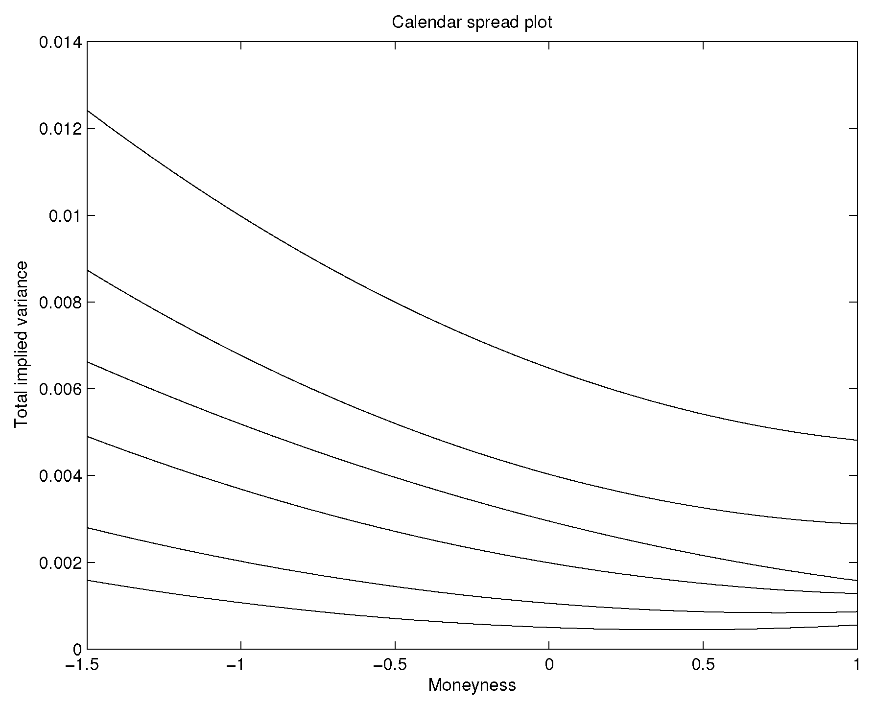
represents the optimal values of $\lambda$ for each of the six different times to maturity. Figure 1 illustrates the plots of total implied variance for all six volatility slices and it shows that total implied variance is an increasing function of time to expiration since the volatility slices never cross each other, so the calibration method eliminates calendar spread arbitrage. Plots for all six Durrleman’s functions are shown separately for each volatility slice in Figure 2. The plots of Durrleman’s function for all six times to maturity are strictly positive around at-the-money, implying the absence of butterfly arbitrage for each volatility slice. Therefore, due to the conditions of Definition 2, we parameterized total implied variance for S&P 500 call option data in such a way that there is no static arbitrage.

To sum up, modeling implied volatility with respect to time to expiration and strike price, and precluding static arbitrage simultaneously, we can be aware of the upcoming price fluctuation of the risky asset and use it to price the options in Equation (6). Therefore, the risk management contract (6) can be priced more precisely based on the behavior of implied volatility. It is necessary to note that we did not implement an algorithm to price the contract since the main focus of this paper is to parametrize implied volatility to improve the precision of contract pricing and the rest is just related to option pricing that is widely studied in the literature.

5. Conclusions

Deposit insurances are introduced after the 1929 Great Depression as a tool to reduce the risk of depositors’ loss. There are two major issues related to deposit insurances: the risk of moral hazard on the one hand, and the risk of miss-pricing and arbitrage on the other hand. The main objective of this study is to focus on the second issue by correctly pricing deposit insurances via improving the implied volatility calibration. As the deposit insurances have been blamed for generating the moral hazard risk, we considered a framework where the risk of moral hazard is ruled out (Assa and Okhrati (2018)) and we focused our attention on arbitrage. In the first step, we showed that in this framework no-arbitrage assumption can be reduced to no-static-arbitrage assumption. This paves the way towards parametrization of the implied volatility. After introducing a quadratic approach to parameterized implied volatility, we mathematically proved that for options with less than one year to maturity and under some special conditions on parameters of the model, there is no opportunity for static arbitrage. The results of the numerical implementation have shown that the proposed quadratic model can be a helpful strategy for modeling implied volatility. Furthermore, our approach improved other quadratic approaches which have already been proposed, since none of them could take care of arbitrage opportunity. Another interesting property of the model is the simplicity of the quadratic function which is understandable by a basic knowledge of mathematics. However, we believe this area of volatility modeling still has some room to improve based on additional market features like the underlying price, time to expiration and strike price, which we leave for future works.