An EM Algorithm for Double-Pareto-Lognormal Generalized Linear Model Applied to Heavy-Tailed Insurance Claims

Abstract

Generalized linear models might not be appropriate when the probability of extreme events is higher than that implied by the normal distribution. Extending the method for estimating the parameters of a double Pareto lognormal distribution (DPLN) in Reed and Jorgensen (2004), we develop an EM algorithm for the heavy-tailed Double-Pareto-lognormal generalized linear model. The DPLN distribution is obtained as a mixture of a lognormal distribution with a double Pareto distribution. In this paper the associated generalized linear model has the location parameter equal to a linear predictor which is used to model insurance claim amounts for various data sets. The performance is compared with those of the generalized beta (of the second kind) and lognorma distributions.

1. Introduction

Heavy-tailed distributions are an important tool for actuaries working in insurance where many insurable events have low likelihoods and high severities and the associated insurance policies require adequate pricing and reserving. In such cases the four-parameter generalized beta distribution of the second kind (GB2) and the three-parameter generalized gamma distribution fulfil this purpose, as demonstrated in McDonald (1990), Wills et al. (2006), Frees and Valdez (2008), Wills et al. (2006), Frees et al. (2014a) and Chapter 9 of Frees et al. (2014b). In fact, the set of possible distributions that could be used for long-tail analyses is much broader than suggested here and good references for these are Chapter 10 of Frees et al. (2014a), Chapter 9 of Frees et al. (2014b) and Section 4.11 of Kleiber and Kotz (2003). We propose in this article the use of the double Pareto lognormal (DPLN) distribution as an alternative model for heavy-tailed events.

The DPLN distribution was introduced by Reed (2003) to model the distribution of incomes. It occurs as the distribution of the stopped wealth where the wealth process is geometric Brownian motion, the initial wealth is lognormally distributed and the random stopping time is exponentially distributed. This parametric model exhibits Paretian behaviour in both tails, among other suitable theoretical properties, and there is favourable evidence of its fit to data in various applications, as demonstrated in Colombi (1990), Reed (2003), Reed and Jorgensen (2004) and Hajargasht and Griffiths (2013) for income data and Giesen et al. (2010) for settlement size data. Particular applications of the DPLN distribution to insurance and actuarial science have previously been given in Ramírez-Cobo et al. (2010) and Hürlimann (2014).

In this paper, the DPLN generalized linear model (GLM) is introduced by setting the location parameter equal to a linear predictor, i.e., $\nu ={\mathit{\beta }}^{\top }\mathit{x}$, where $\mathit{\beta }\in R^d$ is a vector of regression coefficients and $\mathit{x}$ is a vector of explanatory variables. Then the mean of the DPLN GLM is proportional to some exponential transformation of the linear predictor. Then an EM algorithm is developed which solves for the regression parameters.

Particular applications of the DPLN distribution to insurance and actuarial science have previously been given in Ramírez-Cobo et al. (2010) and Hürlimann (2014).  However, another practical application of the DPLN GLM, beyond what is demonstrated in this article, is assessing variability of survival rates of employment, as done in Yamaguchi (1992).

Applying this generalized linear model, we model the claim severity for private passenger automobile insurance and claim amounts due to bodily injuries sustained in car accidents, the data sets of which are supplied in Frees et al. (2014a). We compare this predictive model with the generalized linear model derived from the generalized beta distribution of the second kind (GB2), which has been employed in modelling incomes, for example by McDonald (1990), and in modelling insurance claims, for example by Wills et al. (2006) and Frees and Valdez (2008). The EM algorithm has previously been applied to insurance data, for example in Kocović et al. (2015) , where it is used to explain losses of a fire insurance portfolio in Serbia.

The rest of the paper is organized as follows. Section 2 explains how the DPLN model is applied to regression by setting the location parameter equal to a linear predictor. In Section 3, details of parameter estimation by the method of maximum likelihood using the related normal skew-Laplace (NSL) distribution are provided, where we develop an EM algorithm for such a purpose. Section 4 gives numerical applications of the models to two insurance-related data sets and makes comparisons of fits with the LN and GB2 distributions using the likelihood ratio test and another test for non-nested models due to Vuong (1989). Out-of-sample performances of the models in regards to capital requirements of an insurer are also provided. Section 5 concludes.

2. DPLN Generalized Linear Model

As mentioned previously, the DPLN distribution can be obtained as a randomly stopped geometric Brownian motion whose initial value is lognormally distributed. Therefore, without any mathematical analysis, stopping the geometric Brownian motion at the initial time with probability one will give the lognormal distribution. If the diffusion coefficient of the geometric Brownian motion is set to zero, we have a deterministic geometric motion which is stopped at an exponentially distributed time, giving the PLN distribution. If also the drift coefficient of the geometric Brownian motion is set to zero then the lognormal distribution results. Another degenerate case emerges when the initial value is constant, that is, when its variance is zero, giving the Pareto distribution. This gives us a sensible intuition on the mathematical derivations in this section.

Formally, given a filtered probability space $(\mathrm{\Omega },\underline{\mathcal{F}},{({\mathcal{F}}_t)}_{t\ge 0},P)$, where $\mathrm{\Omega }$ is the sample space, $\underline{\mathcal{F}}$ is the $\sigma$-algebra of events, ${({\mathcal{F}}_t)}_{t\ge 0}$ is the filtration of sub-$\sigma$-algebras of $\underline{\mathcal{F}}$ and P is a probability measure, we consider the adapted stochastic process Y specified by the following stochastic differential equation (SDE), for $t\ge 0$,

$$d{Y}_t=(\mu -\frac{1}{2}{\sigma }^2)dt+\sigma d{W}_t,$$

(1)

where $\mu$ and $\sigma \ge 0$ are constants and W is a Wiener process adapted to the filtration ${(\mathcal{F})}_{t\ge 0}$.

Then for a fixed time $t\ge 0$, the random variable $Y_t$ can be written as

$$Y_t=Y_0+(\mu -\frac{1}{2}{\sigma }^2)t+\sigma W_t.$$

(2)

Now if $Y_0$ is a random variable, dependent upon the vector of predictor variables $\mathit{x}={(x_1,x_2,\dots ,x_d)}^{\top }\in R^d$, such that $Y_0\sim \mathrm{N}(\nu ,{\tau }^2)$, where $\nu ={\mathit{\beta }}^{\top }\mathit{x}$, and if we stop the process Y randomly at time $t=T$, where $T\sim Exp(\lambda )$, then $Y_T$ is a normal skew Laplace (NSL) distributed random variable regressed on the vector of predictors $\mathit{x}$, that is

$$Y_T\sim NSL(\nu ,{\tau }^2,{\lambda }_1,{\lambda }_2),$$

(3)

the exponential of which is a DPLN distributed random variable $V_T$ (see Reed and Jorgensen (2004) for more details) dependent on the same predictors, namely

$$V_T=\exp (Y_T)\sim DPLN(\nu ,{\tau }^2,{\lambda }_1,{\lambda }_2),$$

(4)

where $\nu ={\mathit{\beta }}^{\top }\mathit{x}$. As indicated previously, the particular case of the PLN distribution arises when $\sigma =0$ in (1) and the case of the lognormal distribution (LN) arises when $\mu =0$ and $\sigma =0$ in (1).

The moment generating function (MGF) of $Y_T$ is

$$MG{F}_{Y_T}(s)=MG{F}_{\log X_0}(s)MG{F}_{T_1-T_2}(s),$$

(5)

where $T_1\sim Exp({\lambda }_1)$ and $T_2\sim Exp({\lambda }_2)$ are exponentially distributed random variables with

$$\begin{array}{cc}{\lambda }_1& =\frac{1}{{\sigma }^2}\left[\sqrt{{(\mu -\frac{1}{2}{\sigma }^2)}^2+2\lambda {\sigma }^2}-(\mu -\frac{1}{2}{\sigma }^2)\right],\hfill \\ {\lambda }_2& =\frac{1}{{\sigma }^2}\left[\sqrt{{(\mu -\frac{1}{2}{\sigma }^2)}^2+2\lambda {\sigma }^2}+(\mu -\frac{1}{2}{\sigma }^2)\right],\hfill \end{array}$$

(6)

as given in Reed and Jorgensen (2004). This product of MGFs demonstrates that the NSL distributed random variable $Y_T$ can be expressed as the sum

$$Y_T=\log X_0+T_1-T_2,$$

(7)

where $\log X_0\sim N(\nu ,{\tau }^2)$ and $T_1$ and $T_2$ are as above.

The probability density function (PDF) of $V_T=\exp (Y_T)$, as in (4), is given by

$$\begin{array}{cc}{f}_{V_T}(x)=\hfill & \frac{{\lambda }_1{\lambda }_2}{{\lambda }_1+{\lambda }_2}\frac{1}{x}[\exp \left\{\frac{1}{2}{\tau }^2{\lambda }_1^2-{\lambda }_1(\log x-\nu )\right\}\mathrm{\Phi }\left(\frac{\log x-{\tau }^2{\lambda }_1-\nu }{\tau }\right)\hfill \\ & +\exp \left\{\frac{1}{2}{\tau }^2{\lambda }_2^2-{\lambda }_2(\nu -\log x)\right\}{\mathrm{\Phi }}^c\left(\frac{\log x+{\tau }^2{\lambda }_2-\nu }{\tau }\right)],\hfill \end{array}$$

(8)

also given in Reed (2003). Because we will work with logarithms of DPLN variates we will make use of the PDF of $Y_T$ given by

$$\begin{array}{cc}{f}_{Y_T}(y)=\hfill & \frac{{\lambda }_1{\lambda }_2}{{\lambda }_1+{\lambda }_2}[\exp \left\{\frac{1}{2}{\tau }^2{\lambda }_1^2-{\lambda }_1(y-\nu )\right\}\mathrm{\Phi }\left(\frac{y-{\tau }^2{\lambda }_1-\nu }{\tau }\right)\hfill \\ & +\exp \left\{\frac{1}{2}{\tau }^2{\lambda }_2^2-{\lambda }_2(\nu -y)\right\}{\mathrm{\Phi }}^c\left(\frac{y+{\tau }^2{\lambda }_2-\nu }{\tau }\right)],\hfill \end{array}$$

(9)

where $\mathrm{\Phi }(·)$ and ${\mathrm{\Phi }}^c(·)$ represent the cumulative distribution function and survival function of the standard normal distribution respectively.

Additional properties concerning the moments of the DPLN and asymptotic tail behaviour can be found in Reed (2003). When we incorporate a vector of explanatory variables (or covariates) $\mathit{x}\in R^d$ in our model, the location parameter $\nu$ is set equal to ${\mathit{\beta }}^{\top }\mathit{x}$, where $\mathit{\beta }\in R^d$ is a vector of regression coefficients, and the mean of the response variable is given by

$$E\left[V_T\right|\mathit{x}]=\frac{{\lambda }_1{\lambda }_2}{({\lambda }_1-1)({\lambda }_2+1)}\exp \{{\mathit{\beta }}^{\top }\mathit{x}+\frac{1}{2}{\tau }^2\},$$

(10)

where $\tau ,{\lambda }_2>0$ and ${\lambda }_1>1$. Each regression coefficient can be interpreted as a proportional change in the mean of the response variable per unit change in the corresponding covariate.

For a random sample coming from $V_T$

$$v_1,v_2,\dots ,v_n$$

(11)

and corresponding vectors of covariates ${\mathit{x}}^{(1)},{\mathit{x}}^{(2)},\dots ,{\mathit{x}}^{(n)}$, we will use the maximum likelihood estimation described in the following section to compute the parameters of the DPLN distribution.

3. Maximum Likelihood Estimation of Parameters

3.1. Methods of Estimation

Given the random sample in (11) and corresponding vectors of covariates, there are several ways of estimating parameters, such as moment matching, where such moments exist, and maximum likelihood estimation (MLE). As we are dealing with heavy-tailed distributions, moment matching may not be possible and we therefore resort to maximum likelihood estimation. Maximum likelihood estimators are also preferable since for large samples the estimators are unbiased, efficient and normally distributed. The EM algorithm of Dempster et al. (1977) is one approach to performing MLE of parameters, which we describe in the next section. Another approach is based on the gradient ascent method which we discuss in a subsequent section.

3.2. Application of the EM Algorithm to DPLN Generalized Linear Model

3.2.1. The EM Algorithm for the DPLN GLM

Our task is to obtain maximum likelihood estimates of the parameters of the model $DPLN(\nu ,{\tau }^2,{\lambda }_1,{\lambda }_2)$ using the EM algorithm, which was developed in Dempster et al. (1977). Because an NSL random variable is the logarithm of a DPLN random variable, fitting a DPLN distribution to the observations in (11) is the same as fitting the NSL distribution to the logarithms $y_1,y_2,\dots ,y_n$ of these observations. The EM algorithm starts from an initial estimate of parameter values and sequentially computes refined estimates which increase the value of the log-likelihood function. In the following paragraphs we explain how it is applied to the DPLN distribution.

Suppose that $\mathit{\theta }=(\mathit{\beta },{\tau }^2,{\lambda }_1,{\lambda }_2)$ is an initial estimate of the parameters of the distribution of the random variable Y whose density function is $f_Y$, given in (9). Let ${\mathit{\theta }}^{\prime }$ denote a refined estimate of the parameters of the distribution , that is, an estimate for which the log-likelihood function ℓ exceeds that of the initial estimate $\mathit{\theta }$. In what follows, we demonstrate how to generate a refined estimate for the DPLN GLM. For the refined estimate ${\mathit{\theta }}^{\prime }$, we can write the log-likelihood function as

$$\ell ({\mathit{\theta }}^{\prime })=\sum _{i=1}^n\log f_Y(y_i;{\mathit{\theta }}^{\prime })=\sum _{i=1}^n\log {\int }_{-\infty }^{\infty }{f}_{Y,Z}(y_i,z;{\mathit{\theta }}^{\prime })dz,$$

(12)

where $f_Y(y)$ is the PDF of the random variable Y, $f_{Y,Z}(y,z)$ is the joint density function of the random variables $(Y,Z)$ and where the random variable Z is latent and therefore unobserved. In our case, the random variable Z is a normally distributed random variable having parameters $\nu$ and ${\tau }^2$, as indicated by the random variable $\log X_0$ in (7).

We now give the probability density function $g_i$, for each $i=1,2,\dots ,n$, for the conditional random variable $Z|Y=y_i$ which only depends on the initial estimate $\mathit{\theta }$ of parameters, and not on ${\mathit{\theta }}^{\prime }$, namely

$$g_i(z)=f_{Y,Z}(y_i,z;\mathit{\theta })/f_Y(y_i;\mathit{\theta })=f_{Z|Y=y_i}(z).$$

(13)

We then rewrite (12) as

$$\begin{array}{cc}\ell ({\mathit{\theta }}^{\prime })& ={\sum }_{i=1}^n\log {\int }_{-\infty }^{\infty }{f}_{Y,Z}(y_i,z;{\mathit{\theta }}^{\prime })dz\hfill \\ & ={\sum }_{i=1}^n\log {\int }_{-\infty }^{\infty }\frac{f_{Y,Z}(y_i,z;{\mathit{\theta }}^{\prime })}{g_i(z)}{g}_i(z)dz\hfill \end{array}$$

(14)

and applying Jensen’s inequality $\log E\left[X\right]\ge E\left[\log X\right]$ gives

$$\begin{array}{cc}\ell ({\mathit{\theta }}^{\prime })& ={\sum }_{i=1}^n\log {\int }_{-\infty }^{\infty }\frac{f_{Y,Z}(y_i,z;{\mathit{\theta }}^{\prime })}{g_i(z)}{g}_i(z)dz\hfill \\ & \ge {\sum }_{i=1}^n{\int }_{-\infty }^{\infty }\log \left\{\frac{f_{Y,Z}(y_i,z;{\mathit{\theta }}^{\prime })}{g_i(z)}\right\}{g}_i(z)dz\hfill \\ & ={\sum }_{i=1}^n{\int }_{-\infty }^{\infty }\log \left\{f_{Y,Z}(y_i,z;{\mathit{\theta }}^{\prime })\right\}{g}_i(z)dz\hfill \\ & -{\sum }_{i=1}^n{\int }_{-\infty }^{\infty }\log \left\{g_i(z)\right\}{g}_i(z)dz.\hfill \end{array}$$

(15)

So our maximization of likelihood amounts to maximizing

$$\sum _{i=1}^n{\int }_{-\infty }^{\infty }\log \left\{f_{Y,Z}(y_i,z;{\mathit{\theta }}^{\prime })\right\}{g}_i(z)dz$$

(16)

with respect to ${\mathit{\theta }}^{\prime }$, which is the M-step or maximization-step of the EM algorithm.

In practice, there is an E-step or expectations-step of the algorithm which is performed prior to the M-step, however we continue with the M-step in the next section because this identifies the variables whose expectations are to be computed in the E-step.

3.2.2. M-Step

So we need to maximize (16) with respect to the parameter ${\mathit{\theta }}^{\prime }$. We show how this is done for the double Pareto lognormal distribution by expanding out the terms in (16), giving

$$\begin{array}{c}{\sum }_{i=1}^n{\int }_{-\infty }^{\infty }\log \left\{f_{Y,Z}(y_i,z;{\mathit{\theta }}^{\prime })\right\}{g}_i(z)dz\hfill \\ ={\sum }_{i=1}^n{\int }_{-\infty }^{\infty }\log [\frac{1}{\sqrt{2\pi {({\tau }^{\prime })}^2}}\exp \left(-\frac{{(z-{\nu }_i^{\prime })}^2}{2{({\tau }^{\prime })}^2}\right)\hfill \\ \times \frac{{\lambda }_1^{\prime }{\lambda }_2^{\prime }}{{\lambda }_1^{\prime }+{\lambda }_2^{\prime }}\left\{\begin{array}{cc}\exp ({\lambda }_2^{\prime }(y_i-z)),\hfill & \mathrm{if}z>y_i\hfill \\ \exp (-{\lambda }_1^{\prime }(y_i-z)),\hfill & \mathrm{if}z\le y_i\hfill \end{array}\right.]g_i(z)dz,\hfill \end{array}$$

(17)

which becomes

$$\begin{array}{c}n\log \left(\frac{1}{\sqrt{2\pi {({\tau }^{\prime })}^2}}\right)-\frac{1}{2{({\tau }^{\prime })}^2}{\sum }_{i=1}^n{z}_i^{(2)}+\frac{1}{{({\tau }^{\prime })}^2}{\sum }_{i=1}^n{z}_i{\nu }_i^{\prime }-\frac{1}{2{({\tau }^{\prime })}^2}{\sum }_{i=1}^n{({\nu }_i^{\prime })}^2\hfill \\ +n\log \frac{{\lambda }_1^{\prime }{\lambda }_2^{\prime }}{{\lambda }_1^{\prime }+{\lambda }_2^{\prime }}+{\lambda }_2^{\prime }{\sum }_{i=1}^n{w}_i^{-}-{\lambda }_1^{\prime }{\sum }_{i=1}^n{w}_i^{+},\hfill \end{array}$$

(18)

where

$$\begin{array}{cc}{z}_i& ={\int }_{-\infty }^{\infty }z{g}_i(z)dz,z_i^{(2)}={\int }_{-\infty }^{\infty }{z}^2{g}_i(z)dz,\hfill \\ w_i^{+}& ={\int }_{-\infty }^{\log x_i}(\log x_i-z)g_i(z)dz,w_i^{-}={\int }_{\log x_i}^{\infty }(\log x_i-z)g_i(z)dz.\hfill \end{array}$$

(19)

We arrive at the following Theorem giving the optimum parameter vector ${\mathit{\theta }}^{\prime }$ and whose proof follows the reasoning for the simpler case without explanatory variables given in Reed and Jorgensen (2004).

Theorem 1.

The components of the parameter vector ${\mathit{\theta }}^{\prime }$ which maximise (16) are

$$\begin{array}{cc}{\mathit{\beta }}^{\prime }\hfill & ={(\mathit{X}{\mathit{X}}^{\top })}^{-1}\mathit{X}\mathit{Z},{({\tau }^{\prime })}^2=\frac{1}{n}\left({\mathbf{1}}^{\top }{\mathit{Z}}^{(2)}-{\mathit{Z}}^{\top }{\mathit{X}}^{\top }{(\mathit{X}{\mathit{X}}^{\top })}^{-1}\mathit{X}\mathit{Z}\right),\hfill \\ {\lambda }_1^{\prime }\hfill & =\frac{1}{P^{\prime }+\sqrt{P^{\prime }{Q}^{\prime }}},{\lambda }_2^{\prime }=\frac{1}{Q^{\prime }+\sqrt{P^{\prime }{Q}^{\prime }}},\hfill \end{array}$$

(20)

where

$$P^{\prime }=\frac{1}{n}\sum _{i=1}^n{w}_i^{+},Q^{\prime }=-\frac{1}{n}\sum _{i=1}^n{w}_i^{-},$$

(21)

$$\mathit{Z}={(z_1,z_2,\dots ,z_n)}^{\top },{\mathit{Z}}^{(2)}={(z_1^{(2)},z_2^{(2)},\dots ,z_n^{(2)})}^{\top }$$

(22)

and $\mathit{X}$ is the matrix of predictor variables

$$\mathit{X}=\left(\begin{array}{cccc}{\mathit{x}}^{(1)}& {\mathit{x}}^{(2)}& \dots & {\mathit{x}}^{(n)}\end{array}\right).$$

(23)

Proof. 

See Appendix A.1. ☐

3.2.3. E-Step

Here we compute the conditional distributions which are used in the E-step. For the set of n logarithms $y_1,\dots ,y_n$ of observations, the maximum likelihood estimates of the parameters can be obtained using the EM algorithm with as follows,

$$g_i(z)=\frac{f_Z(z;\mathit{\theta })f_W(y_i-z;\mathit{\theta })}{f_Y(y_i;\mathit{\theta })},$$

(24)

where the density functions $f_Z$, $f_W$ and $f_Y$ are defined as

$$\begin{array}{cc}{f}_Z(z;\mathit{\theta })& =\frac{1}{\sqrt{2\pi {\tau }^2}}\exp \left\{-\frac{1}{2{\tau }^2}{(z-\nu )}^2\right\},\hfill \\ f_W(w;\mathit{\theta })& =\frac{{\lambda }_1{\lambda }_2}{{\lambda }_1+{\lambda }_2}\left\{\begin{array}{cc}\exp ({\lambda }_{2}w)\hfill & w<0\hfill \\ \exp (-{\lambda }_{1}w)\hfill & w\ge 0\hfill \end{array}\right.\hfill \\ f_Y(y;\mathit{\theta })& =\varphi \left((y-\nu )/\tau \right)\left\{R({\lambda }_1\tau -(y-\nu )/\tau )+R({\lambda }_2\tau +(y-\nu )/\tau )\right\}.\hfill \end{array}$$

(25)

For this choice of $g_i$, $\log f_{Y,Z}(y_i,z;{\mathit{\theta }}^{\prime })$ in (16) becomes

$$\log f_{Y,Z}(y_i,z;{\mathit{\theta }}^{\prime })=\log f_Z(z;{\mathit{\theta }}^{\prime })+\log f_W(y_i-z;{\mathit{\theta }}^{\prime }).$$

(26)

Our E-step of the EM algorithm is given in the following Theorem, most of the equations of which are mentioned in Reed and Jorgensen (2004) but for which we supply explicit proofs.

Theorem 2.

The expectations in our E-step are as follows

$$\begin{array}{cc}{z}_i& ={\int }_{-\infty }^{\infty }z{g}_i(z)dz=\nu +{\tau }^2\frac{{\lambda }_{1}R(p_i)-{\lambda }_{2}R(q_i)}{R(p_i)+R(q_i)},\hfill \\ z_i^{(2)}& ={\int }_{-\infty }^{\infty }{z}^2{g}_i(z)dz={\nu }^2+{\tau }^2-{\tau }^2\frac{p_i+q_i}{R(p_i)+R(q_i)}\hfill \\ & +{\tau }^2\frac{(2\nu {\lambda }_1+{\lambda }_1^2{\tau }^2)R(p_i)+({\lambda }_2^2{\tau }^2-2\nu {\lambda }_2)R(q_i)}{R(p_i)+R(q_i)},\hfill \\ w_i^{+}& ={\int }_{-\infty }^{y_i}(y_i-z)g_i(z)dz=\tau \frac{-p_{i}R(p_i)+1}{R(p_i)+R(q_i)},\hfill \\ w_i^{-}& ={\int }_{y_i}^{\infty }(y_i-z)g_i(z)dz=\tau \frac{q_{i}R(q_i)-1}{R(p_i)+R(q_i)},\hfill \end{array}$$

(27)

where $p_i=-(y_i-\nu )/\tau +{\lambda }_1\tau$ and $q_i=(y_i-\nu )/\tau +{\lambda }_2\tau$.

Proof. 

See Appendix A.2. ☐

3.2.4. Standard Errors

The standard errors of the estimates $\widehat{\mathit{\theta }}=({\widehat{\mathit{\beta }}}^{\top },{\widehat{\tau }}^2,{\widehat{\lambda }}_1,{\widehat{\lambda }}_2)$ can be estimated in the last iteration of the EM algorithm, as shown in Louis (1982). The observed Fisher information matrix evaluated at $\widehat{\mathit{\theta }}$ based on the observations ${\left\{v_i\right\}}_{i=1}^n$ can be approximated by

$$\mathcal{I}(\widehat{\mathit{\theta }};v_i)\approx \sum _{i=1}^n\frac{\partial }{\partial \mathit{\theta }}\log f_Y(\log v_i;\widehat{\mathit{\theta }}){\left[\frac{\partial }{\partial \mathit{\theta }}\log f_Y(\log v_i;\widehat{\mathit{\theta }})\right]}^{\top },$$

(28)

where $f_Y$ is as in (9). Since $E\left[\frac{\partial }{\partial \mathit{\theta }}\log f_Y(y_i;\mathit{\theta })|y_i;\widehat{\mathit{\theta }}\right]=\frac{\partial }{\partial \mathit{\theta }}\log f_Y(y_i;\widehat{\mathit{\theta }})$, (28) is equivalent to

$$\sum _{i=1}^n\frac{\partial }{\partial \mathit{\theta }}E\left[\log f_Y(y_i;\mathit{\theta })|y_i;\widehat{\mathit{\theta }}\right]{\left(\frac{\partial }{\partial \mathit{\theta }}E\left[\log f_Y(y_i;\mathit{\theta })|y_i;\widehat{\mathit{\theta }}\right]\right)}^{\top }.$$

In particular,

$$\begin{array}{c}\hfill {\displaystyle \frac{\partial }{\partial \mathit{\theta }}E\left[\log f_Y(y_i;\mathit{\theta })\right]}\\ =& {\left(\frac{\partial E\left[\log f(u_i;{\nu }_i,\tau )|y_i;\widehat{\mathit{\theta }}\right]}{\partial {(\mathit{\beta },\tau )}^{\top }},\frac{\partial E\left[\log f_Y(w_i;{\lambda }_1,{\lambda }_2)|y_i;\widehat{\mathit{\theta }}\right]}{\partial {({\lambda }_1,{\lambda }_2)}^{\top }}\right)}^{\top },\hfill \end{array}$$

and therefore these expressions are available in the last iteration of the EM algorithm.

3.3. Gradient Ascent Method

The gradient ascent method is applied to the likelihood function of the normal skew Laplace distribution in this subsection. Let be $\mathit{y}=(y_1,\dots ,y_n)$ be a random sample of size n from a NSL distribution. Its log-likelihood function is:

$$\begin{array}{c}{\displaystyle \ell (\mathit{y};\mathit{\beta },{\tau }^2,{\lambda }_1,{\lambda }_2)=n\log {\lambda }_1+n\log {\lambda }_2-n\log ({\lambda }_1+{\lambda }_2)}\\ +\sum _{i=1}^n\log \left(\frac{\mathrm{\Phi }\left(\frac{y_i-{\tau }^2{\lambda }_1-{\nu }_i}{\tau }\right)}{\exp \{-\frac{1}{2}{\lambda }_1{\tau }^2+{\lambda }_1(y_i-{\nu }_i)\}}+\frac{1-\mathrm{\Phi }\left(\frac{y_i+{\tau }^2{\lambda }_2-{\nu }_i}{\tau }\right)}{\exp \{-\frac{1}{2}{\lambda }_2{\tau }^2+{\lambda }_2({\nu }_i-y_i)\}}\right).\end{array}$$

(29)

The solutions of the $d+3$ score equations that are shown in the Appendix, provide the maximum likelihood estimates of ${\lambda }_1$, ${\lambda }_2$, $\tau$ and ${\left\{{\mathit{\beta }}_j\right\}}_{j=1,\cdots ,d}$, which can be obtained by numerical methods such as Newton-Raphson algorithm. Alternatively, parameter estimates can be obtained directly via a grid search for the global maximum of the log-likelihood surface given by (29), or equivalently by maximizing the log-likelihood function derived from the expression (8). We have used FindMaximum function of Mathematica software package v.11.0. Since the global maximum of the log-likelihood surface is not guaranteed, different initial values of the parametric space can be considered as seed point using different methods of maximization, such as Newton–Raphson method, Principal Axis method and the Broyden–Fletcher–Goldfarb–Shanno algorithm (BGGS), among others. The standard errors of the estimates have been approximated by inverting the Hessian matrix and the relevant partial derivatives can be approximated well by finite differences.

4. Numerical Applications

In this section, two well-known data sets in the actuarial literature that can be downloaded from Professor E. Frees’ personal website1 will be considered to test the practical performance of the DPLN generalized linear model. For the two data sets considered, the EM algorithm for the DPLN GLM was stopped when the relative change of the log-likelihood function was smaller than $1\times {10}^{-10}$. The initial values were calculated by using the estimates of the lognormal GLM and the estimates of the parameters ${\lambda }_1$ and ${\lambda }_2$ for the model without covariates.

Because we are comparing the DPLN generalized linear model with the GB2 GLM, we give here some rudimentary facts concerning the GB2 distribution. Let Z be a random variable having the $Beta(p,q)$ distribution, for $p,q\in (0,\infty )$, as defined in Chapter 6 of Kleiber and Kotz (2003). Then, for $\nu \in (-\infty ,\infty )$ and $\tau \in (0,\infty )$, the random variable

$$V=\exp (\nu ){(Z/(1-Z))}^{\tau }$$

(30)

has the GB2 distribution and its probability density function can be written as

$$f_V(v)=\frac{\exp \left\{\frac{p(\log v-\nu )}{\tau }\right\}}{v\tau B(p,q){[1+\exp \left\{\frac{(\log v-\nu )}{\tau }\right\}]}^{p+q}},$$

(31)

where $v\in (0,\infty )$, $\nu$ is a location parameter, $\tau >0$ is a scale parameter, $p>0$ and $q>0$ are shape parameters and

$$B(p,q)={\int }_0^1{z}^{p-1}{(1-z)}^{q-1}dz=\Gamma (p)\Gamma (q)/\Gamma (p+q)$$

is the Beta function. As for the aformentioned distributions, to include explanatory variables in the model, we let the location parameter be a linear function of covariates, i.e., $\nu ={\mathit{\beta }}^{\top }\mathit{x}$. The k-th moment is easily seen to be

$$E\left[V^k\right]=\exp (k\nu )\frac{B(p+k\tau ,q-k\tau )}{B(p,q)},$$

(32)

where $k\in (-p/\tau ,q/\tau )$, and looking at the case $k=1$ we can interpret each of the regression coefficients ${\mathit{\beta }}_i$, $i=1,\dots ,d$, as being the proportional sensitivity of the mean to the corresponding covariate. Further details of this model can be found in Frees et al. (2014a). Parameter estimation for the GB2 GLM has been performed via a grid search for the global maximum of the log-likelihood surface associated to this model. We have used FindMaximum function of Mathematica software package v.11.0.

4.1. Example 1: Automobile Insurance

The first data set pertains to claims experience from a large midwestern (US) property and casualty insurer for private passenger automobile insurance.

The dependent variable is the amount paid on a closed claim, in US$. The sample includes 6773 claims. The following explanatory variables have been considered to explain the claims amount:

• GENDER, gender of operator, takes the value 1 if female and 0 otherwise;
• AGE, age of operator;
• CLASS rating class of operator as coded in

  Table 1. Parameter estimates, standard errors (S.E.) and p-values of the t-test for automobile insurance claims dataset under lognormal distribution (LN), generalized beta distribution of the second kind (GB2) and double Pareto lognormal distribution (DPLN) generalized linear models.

  	Generalized Linear Model
  Estimate (S.E.)	LN	GB2	DPLN
  INTERCEPT	7.184 (0.150)	7.234 (0.163)	7.260 (0.080)
  p-value	<0.0001	<0.0001	<0.0001
  GENDER	−0.035 (0.027)	−0.012 (0.027)	−0.039 (0.014)
  p-value	0.1918	0.6604	0.0073
  AGE	−0.004 (0.002)	−0.004 (0.002)	−0.005 (0.001)
  p-value	0.0167	0.0110	<0.0001
  C1	0.018 (0.118)	−0.002 (0.115)	0.017 (0.063)
  p-value	0.8760	0.9877	0.7889
  C11	0.063 (0.116)	0.021 (0.114)	0.063 (0.062)
  p-value	0.5853	0.8567	0.3146
  C1A	−0.076 (0.165)	−0.047 (0.161)	−0.085 (0.088)
  p-value	0.6453	0.7687	0.3389
  C1B	0.057 (0.122)	0.008 (0.120)	0.055 (0.066)
  p-value	0.6411	0.9471	0.4045
  C1C	−0.164 (0.206)	−0.154 (0.203)	−0.1392 (0.110)
  p-value	0.4267	0.4498	0.2075
  C2	−0.134 (0.176)	0.034 (0.170)	−0.132 (0.094)
  p-value	0.4450	0.8407	0.1626
  C6	0.070 (0.120)	0.033 (0.118)	0.086 (0.065)
  p-value	0.5594	0.7767	0.1815
  C7	−0.030 (0.116)	−0.028 (0.114)	−0.033 (0.062)
  p-value	0.7983	0.8071	0.5960
  C71	0.018 (0.115)	−0.029 (0.113)	0.013 (0.062)
  p-value	0.8725	0.7941	0.8380
  C72	0.239 (0.160)	0.036 (0.157)	0.226 (0.086)
  p-value	0.1367	0.8203	0.0087
  C7A	0.127 (0.150)	0.225 (0.147)	0.123 (0.080)
  p-value	0.3965	0.1249	0.1248
  C7B	0.128 (0.118)	0.091 (0.116)	0.129 (0.063)
  p-value	0.2806	0.4313	0.042
  C7C	0.282 (0.162)	0.173 (0.158)	0.270 (0.087)
  p-value	0.0824	0.2735	0.0020
  F1	0.103 (0.228)	−0.134 (0.222)	0.132 (0.122)
  p-value	0.6499	0.5462	0.2785
  F11	−0.087 (0.203)	−0.177 (0.202)	−0.099 (0.109)
  p-value	0.6675	0.3798	0.3623
  F6	0.058 (0.144)	0.069 (0.142)	0.090 (0.077)
  p-value	0.6880	0.6300	0.2434
  F7	−0.347 (0.178)	−0.382 (0.172)	−0.351 (0.095)
  p-value	0.0508	0.0266	0.0002
  $\tau$	1.068 (0.009)	0.968 (0.111)	0.810 (0.006)
  p-value	<0.0001	<0.0001	<0.0001
  p or ${\lambda }_1$		2.083 (0.371)	2.127 (0.032)
  p-value		<0.0001	<0.0001
  q or ${\lambda }_2$		2.109 (0.427)	1.952 (0.029)
  p-value		0.0001	<0.0001
  NLL	57,164.4	57,145.2	57,139.3
  AIC	11,4370.7	11,4336.6	11,4324.6
  BIC	114,513.9	114,493.2	114,481.6
  CT	3.0108	95.4570	91.1358

  .

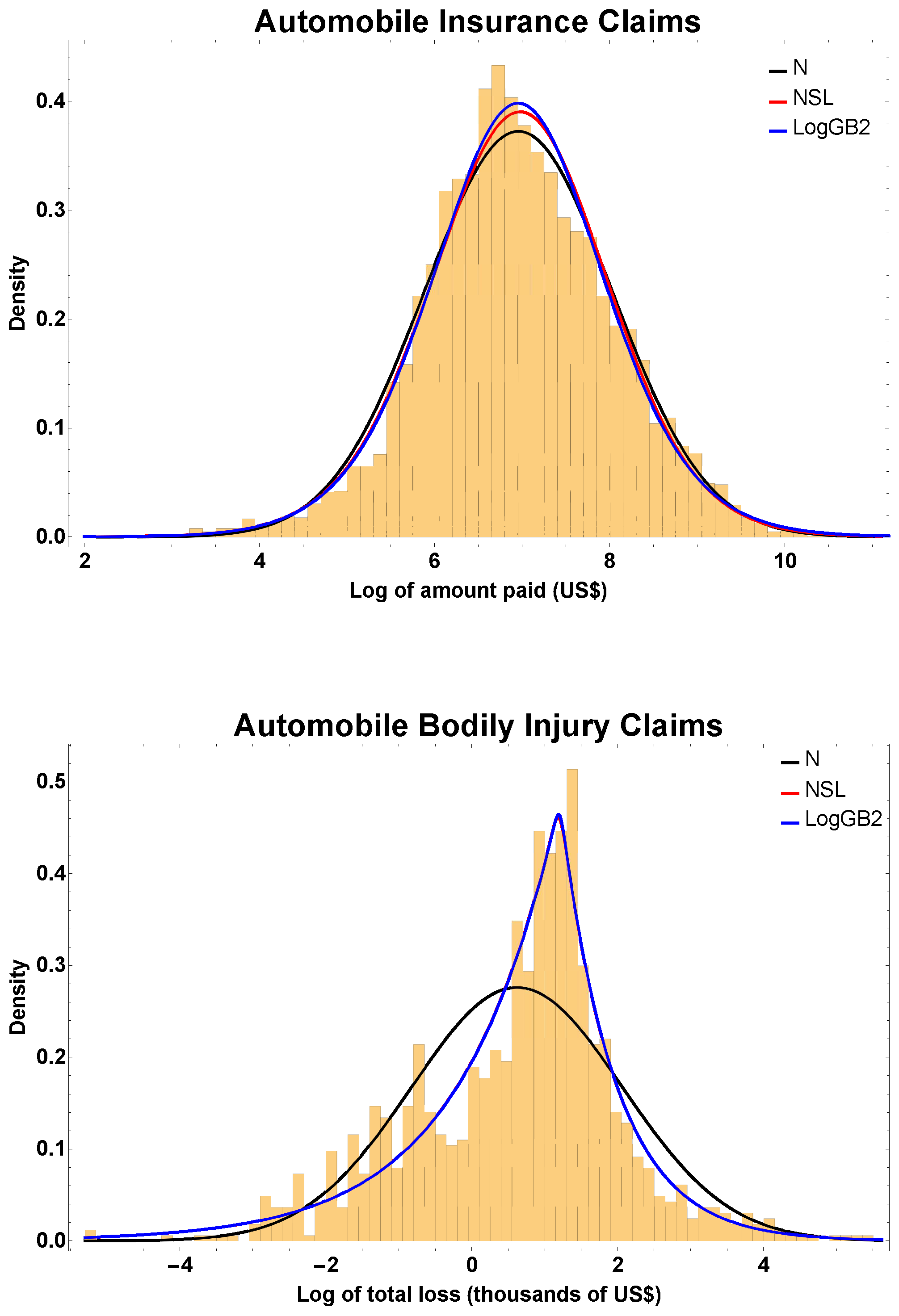
In the top part of Figure 1 the histogram of the Automobile insurance claims is exhibited in logarithmic scale. This dataset is quite symmetrical but it presents a slightly longer lower tail. For that reason the DPLN distribution seems suitable to explain this dataset.

4.1.1. Model Without Covariates

Here, for comparison purposes only, the lognormal, DPLN and GB2 distributions will be used to describe the total losses (e.g., when explanatory variables are not considered). Firstly, the automobile insurance claims dataset is examined.

Table 2. Model fitting results of the LN, GB2 and DPLN distributions regarding automobile insurance claims.

	Distribution
Estimate (S.E.)	LN	GB2	DPLN
$\nu$	$6.956(0.013)$	$6.945(0.074)$	$7.009(0.007)$
$\tau$	$1.071(0.009)$	$0.916(0.089)$	$0.824(0.006)$
p or ${\lambda }_1$		$1.914(0.289)$	$2.191(0.033)$
q or ${\lambda }_2$		1.897 (0.316)	$1.961(0.029)$
NLL	57,185.1	57,162.5	57,161.5
AIC	114,374	114,333	114,331
BIC	114,390	114,360	114,358
CT	0.2340	3.8376	12.5113

summarizes parameters estimates obtained by maximum likelihood with corresponding standard errors (in brackets) for the aforementioned distributions.

In respect of model selection, we also provide the negative of the maximum of the log-likelihood (NLL), Akaike’s information criterion (AIC) and Bayesian information criterion (BIC) results in the table. Note that for all three measures of model validation, smaller values indicate a better fit of the model to the empirical data. As expected, the lognormal distribution exhibits the worst performance in terms of all three measures of model validation. In the top part of Figure 2, we have superimposed the log transformation of these three distributions to the empirical distribution of the log of the claims sizes to test the fit in both tails. It is evident that the log transformation of the lognormal distribution (black curve), i.e., Normal distribution (N), provides the worst fit due to asymmetry of the data. The logGB2 (blue curve) and NSL distributions (red curve) give better fit to data as measured by the NLL, AIC and BIC, although the latter model adheres closely to the data. Although it is not shown in Table 2, the PLN distribution, replicates the fit of the LN distribution and the value of the shape parameter that controls the right tail tends to infinity. The computing times (CT) in seconds to estimate the maximum likelihood estimates by directly maximizing the log-likelihood surface for these distributions are shown in the last row of the table. The computing time of the EM algorithm for the DPLN GLM was 1145.86 s using the stopping criterion that the relative change of the log-likelihood function be less than $1\times {10}^{-4}$.

4.1.2. Comparison of Estimation from Simulations

In this section we compare the methods of estimating parameters by conducting the following simulation experiment. For the lognormal, DPLN and GB2 distributions, we simulate values based on the corresponding parameter estimates given in Table 2, and then, using as appropriate either standard formulae or the EM algorithm, compute parameter estimates from the 1000 simulated data sets of size $N=100,200,300,400,500,1000$. The results are shown in

Table 3. Results of the simulation experiment involving 1000 simulations of data sets of size N, with standard errors shown in brackets.

	Distribution
Sample Size $\mathit{N}$	LN	DPLN	GB2
100	$\widehat{\nu }=6.9551$ ($0.1017$)	$\widehat{\nu }=7.0095$ ($0.1401$)	$\widehat{\nu }=7.0670$ ($2.1561$)
	$\widehat{\tau }=1.0599$ ($0.0779$)	$\widehat{\tau }=0.8091$ ($0.1063$)	$\widehat{\tau }=1.3188$ ($6.6295$)
		${\widehat{\lambda }}_1=2.3715$ ($0.5056$)	$\widehat{p}=146.9750$ ($2403.6500$)
		${\widehat{\lambda }}_2=2.1121$ ($0.4517$)	$\widehat{q}=180.7270$ ($3075.6600$)
200	$\widehat{\nu }=6.9565$ ($0.0763$)	$\widehat{\nu }=7.0098$ ($0.1015$)	$\widehat{\nu }=6.9789$ ($0.5097$)
	$\widehat{\tau }=1.0684$ ($0.0540$)	$\widehat{\tau }=0.8176$ ($0.0750$)	$\widehat{\tau }=0.5591$ ($1.7972$)
		${\widehat{\lambda }}_1=2.3024$ ($0.3785$)	$\widehat{p}=11.3055$ ($204.7950$)
		${\widehat{\lambda }}_2=2.0471$ ($0.3450$)	$\widehat{q}=12.6484$ ($231.6380$)
300	$\widehat{\nu }=6.9569$ ($0.0610$)	$\widehat{\nu }=7.0038$ ($0.0859$)	$\widehat{\nu }=6.9602$ ($0.5468$)
	$\widehat{\tau }=1.0668$ ($0.0445$)	$\widehat{\tau }=0.8235$ ($0.0636$)	$\widehat{\tau }=0.3635$ ($0.3605$)
		${\widehat{\lambda }}_1=2.2636$ ($0.3131$)	$\widehat{p}=1.0887$ ($5.1770$)
		${\widehat{\lambda }}_2=2.0389$ ($0.2892$)	$\widehat{q}=1.7380$ ($26.1729$)
400	$\widehat{\nu }=6.9578$ ($0.0531$)	$\widehat{\nu }=7.0031$ ($0.0772$)	$\widehat{\nu }=6.9411$ ($0.2291$)
	$\widehat{\tau }=1.0695$ ($0.0368$)	$\widehat{\tau }=0.8211$ ($0.0560$)	$\widehat{\tau }=0.3052$ ($0.2085$)
		${\widehat{\lambda }}_1=2.2368$ ($0.2761$)	$\widehat{p}=0.7963$ ($4.7610$)
		${\widehat{\lambda }}_2=2.0189$ ($0.2553$)	$\widehat{q}=0.6528$ ($0.7841$)
500	$\widehat{\nu }=6.9555$ ($0.0465$)	$\widehat{\nu }=7.0104$ ($0.0665$)	$\widehat{\nu }=6.9409$ ($0.0843$)
	$\widehat{\tau }=1.0709$ ($0.0333$)	$\widehat{\tau }=0.8208$ ($0.0489$)	$\widehat{\tau }=0.2941$ ($0.1768$)
		${\widehat{\lambda }}_1=2.2289$ ($0.2450$)	$\widehat{p}=0.6268$ ($0.4547$)
		${\widehat{\lambda }}_2=1.9930$ ($0.2162$)	$\widehat{q}=0.6036$ ($0.4101$)
1000	$\widehat{\nu }=6.9553$ ($0.0335$)	$\widehat{\nu }=7.0077$ ($0.0488$)	$\widehat{\nu }=6.9493$ ($0.0526$)
	$\widehat{\tau }=1.0699$ ($0.0242$)	$\widehat{\tau }=0.8208$ ($0.0358$)	$\widehat{\tau }=0.2680$ ($0.1085$)
		${\widehat{\lambda }}_1=2.2055$ ($0.1776$)	$\widehat{p}=0.5409$ ($0.2539$)
		${\widehat{\lambda }}_2=1.9722$ ($0.1558$)	$\widehat{q}=0.5344$ ($0.2460$)

, where it is evident that increasing the sample size increases the accuracy of the parameter estimate. Of course, the true parameter values are given in Table 2, and these are the limits of the estimates as the sample size N increases. Importantly, the standard errors of the parameter estimates in Table 3 are noticeably smaller for the DPLN distribution, highlighting the consistency of the parameter estimation for the DPLN model. It is noteworthy to observe that the parameter estimates of the GB2 distribution are unstable for small sample sizes, which is not the case for the DPLN model. This highlights an advantage of the DPLN model over the GB2 in this case.

4.1.3. Including Explanatory Variables

Making use of the above additional information, we aim to better explain the total losses in terms of the set of covariates by using the DPLN generalized linear model. For the purpose of comparison, we have also fitted the lognormal and GB2 generalized linear models. Here, we choose the identity link function for the location parameter.

From left to right in Table 1, the parameter estimates, standard errors (S.E.) and the corresponding p-values calculated based on the t-Wald statistics for the LN, GB2 and DPLN generalized linear models are displayed for the automobile insurance claims dataset. The AIC and BIC values for each model are provided in the last two rows of the table. For the i-th claimant, the number of total amount $y_i$ follows (10) whose mean depends on the above set of covariates through the identity link function. The exponential of INTERCEPT coefficient 7.260 is proportional to the predicted loss amount when the values of the other explanatory variables are equal to 0. This estimate is statistically significant at the usual significance levels, i.e., 5% and 1%. In total, the estimates of 10 out of 23 parameters for the DPLN generalized linear models are statistically significant at the usual levels (i.e., 5% and 1%) including the scale and shape parameters. The results for the LN and GB2 generalized linear model are also exhibited in Table 1 to compare their behaviour with DPLN generalized linear model. As it can be seen the fit provided by the DPLN generalized linear model improves the one provided by GB2. For the DPLN generalized linear model, parameters were estimated by the method of maximum likelihood by maximizing the log-likelihood surface. The same estimates were achieved by the EM algorithm described in Section 3.2. The standard errors of the parameter estimates for the DPLN GLM were computed from the last iteration of the EM algorithm and also approximated by inverting the Hessian matrix. Similar values were obtained. The computing times in seconds to estimate the maximum likelihood estimates by directly maximizing the log-likelihood surface for these generalized linear models are shown in the last row of the table. The DPLN GLM shows a better performance than the GB2 counterpart. The computing time of the EM algorithm for the DPLN GLM was 2239.24 s using the stopping criterion that the relative change of the log-likelihood function be less than $1\times {10}^{-4}$.

4.1.4. Model Validation

Now, we analyze model validation from a practical perspective. In this regard, LN generalized linear model can be seen as a limiting case of DPLN generalized linear model when both ${\lambda }_1$ and ${\lambda }_2$ tend to infinity. We are interested, by means of the likelihood ratio test, in determining whether the LN generalized linear model (null hypothesis) is preferable to DPLN generalized linear model (alternative hypothesis) in describing these datasets. The test statistic is $T=2({\ell }_{LN}-{\ell }_{DPLN})$ where ${\ell }_{LN}$ and ${\ell }_{DPLN}$ represent the maximum of the log-likelihood function for the LN and DPLN generalized linear models respectively. Asymptotically, under certain regularity conditions (see for example Lehmann and Casella (1998)) T follows a chi-square distribution with two degrees of freedom. We have that $T=2(-57179.69+57155.87)=50.02$, therefore the larger model (DPLN) is preferable to the smaller (LN) generalized linear model at the usual significance levels, i.e., 5% and 1% (p-value less than 0.0001).

Next, the likelihood ratio test proposed by Vuong (1989) for non-nested models will be considered as a tool for model diagnostic. The test statistic is

$$\begin{array}{c}\hfill T=\frac{1}{\omega \sqrt{n}}\left({\ell }_f({\widehat{\mathit{\theta }}}_1)-{\ell }_g({\widehat{\mathit{\theta }}}_2)-\log n\left(\frac{n_f}{2}-\frac{n_g}{2}\right)\right),\end{array}$$

where

$$\begin{array}{c}\hfill {\omega }^2=\frac{1}{n}\sum _{i=1}^n{\left[\log \left(\frac{f({\widehat{\mathit{\theta }}}_1)}{g({\widehat{\mathit{\theta }}}_2)}\right)\right]}^2-{\left[\frac{1}{n}\sum _{i=1}^n\log \left(\frac{f({\widehat{\mathit{\theta }}}_1)}{g({\widehat{\mathit{\theta }}}_2)}\right)\right]}^2\end{array}$$

is the sample variance of the pointwise log-likelihood ratios and f and g represent the probability density function (pdf) of two different non–nested models, ${\widehat{\mathit{\theta }}}_1$ and ${\widehat{\mathit{\theta }}}_2$ are the maximum likelihood estimates of ${\mathit{\theta }}_1$ and ${\mathit{\theta }}_2$ and $n_f$ and $n_g$ are the number of estimated coefficients in the model with pdf f and g respectively. Note that the Vuong’s statistic is sensitive to the number of estimated parameters in each model and therefore the test must be corrected for dimensionality. Under the null hypotheses, $H_0:E[{\ell }_f({\widehat{\mathit{\theta }}}_1)-{\ell }_g({\widehat{\mathit{\theta }}}_2)]=0$ and T is asymptotically normally distributed. At the 5% significance level, the rejection region for this test in favor of the alternative hypothesis occurs when $T>1.96$.

Now we compare the GB2 and DPLN generalized linear models in terms of Vuong’s test. Under the null hypothesis the two models are equally close to the true but unknown specification. For our data set, the value of the test statistic is $T=1.00$ and we fail to reject $H_0$, and therefore differences between these two models do not exist.

4.2. Example 2: Automobile Bodily Injury Claims

The second data set deals with automobile bodily injury claims sourced from the Insurance Research Council (IRC), a division of the American Institute for Chartered Property Casualty Underwriters and the Insurance Institute of America. The data, collected in 2002, contains demographic information about the claimants, attorney involvement and the economic losses (in thousands of US$), among other variables. As some of these explanatory variables contain missing observations, we only consider those data items having no missing values, resulting in a sample of 1,091 losses from a single state. We use as the response variable the claimant’s total economic loss. Also, additional information is available to explain the claimants’ total economic losses. We employ the following factors as covariates in our model fitting:

• ATTORNEY, takes the value 1 if the claimant is represented by an attorney and 0 otherwise;
• CLMSEX, takes the value 1 if the claimant is male and 0 otherwise;
• MARRIED, takes the value 1 if the claimant is married and 0 otherwise;
• SINGLE, takes the value 1 if the claimant is single and 0 otherwise;
• WIDOWED, takes the value 1 if the claimant is widowed and 0 otherwise;
• CLMINSUR, whether or not the claimant’s vehicle was uninsured ($=1$ if yes and 0 otherwise);
• SEATBELT, whether or not the claimant was wearing the seatbelt/child restraint ing belt’s vehicle was uninsured ($=1$ if yes and 0 otherwise);
• CLMAGE, claimant’s age.

The empirical distribution of this variable combines losses of small, moderate and large sizes which makes it suitable for fitting heavy-tailed distributions. It has other features such as unimodality, skewness and a long upper tail, indicating a high likelihood of extremely expensive events. In the bottom part of Figure 1 the histogram of the response variable of this data set is shown again in logarithmic scale. A heavy lower tail is evident when this scale is used.

4.2.1. Model Without Covariates

The results for the bodily injury claims data are shown in

Table 4. Results of fitting the LN, GB2 and DPLN distributions to automobile bodily injury claims data.

	Distribution
Estimate (S.E.)	LN	GB2	DPLN
$\nu$	$0.620(0.044)$	$1.204(0.052)$	$1.200(0.040)$
$\tau$	$1.445(0.031)$	$0.022(0.186)$	$0.047(0.150)$
p or ${\lambda }_1$		$0.017(0.140)$	$1.324(0.068)$
q or ${\lambda }_2$		$0.030(0.247)$	$0.749(0.025)$
NLL	2626.74	2573.47	2573.47
AIC	5257.48	5154.94	5154.94
BIC	5267.47	5174.92	5174.92
CT	0.1716	3.4476	3.0888

. The GB2 and DPLN distributions give the best fit to data as measured by these three measures of model selection. As expected, the LN distribution has the worst performance due to the asymmetry of the data. Again, although it is not shown in Table 4, the three-parameter PLN model replicates the LN distribution. This is due to the fact that the former model is a limiting case of the latter when shape parameter ${\lambda }_1$ tends to infinity. These results are also supported by the bottom part of Figure 1, where it can be seen that the log transformation of the GB2 distribution $Log$GB2 (blue curve) and the NSL distribution (red curve) provide almost an identical fit to data. The MLEs for the DPLN distribution were obtained by using the EM algorithm whose starting parameter values ${\lambda }_1$, ${\lambda }_2$, $\nu$ and $\tau$ are those obtained by moment-matching the first four cumulants. These MLEs were confirmed by those obtained directly from maximizing the log-likelihood surface. The computing times in seconds to estimate the maximum likelihood estimates by directly maximizing the log-likelihood surface for these distributions are shown in the last row of the table. The computing time of the EM algorithm for the DPLN GLM was 1,322.81 seconds using the stopping criterion that the relative change of the log-likelihood function be less than $1\times {10}^{-4}$.

4.2.2. Comparison of Estimation from Simulations

In this section we compare the methods of estimating parameters by conducting the following simulation experiment. For the lognormal and DPLN distributions, we simulate values based on the corresponding parameter estimates given in Table 4, and then, using as appropriate either standard formulae or the EM algorithm, compute parameter estimates from the 1000 simulated data sets of size $N=100,200,300,400,500,1000$. The results are shown in

Table 5. Results of the simulation experiment involving 1000 simulations of data sets of size N, with standard errors shown in brackets.

	Distribution
Sample Size $\mathit{N}$	LN	DPLN
100	$\widehat{\nu }=0.6220$ ($0.1442$)	$\widehat{\nu }=1.2001$ ($0.0028$)
	$\widehat{\tau }=1.4336$ ($0.1054$)	$\widehat{\tau }=0.0470$ ($0.0004$)
		${\widehat{\lambda }}_1=1.3611$ ($0.1934$)
		${\widehat{\lambda }}_2=0.7663$ ($0.0861$)
200	$\widehat{\nu }=0.6214$ ($0.0995$)	$\widehat{\nu }=1.2001$ ($0.0020$)
	$\widehat{\tau }=1.4397$ ($0.0714$)	$\widehat{\tau }=0.0470$ ($0.0002$)
		${\widehat{\lambda }}_1=1.3472$ ($0.1379$)
		${\widehat{\lambda }}_2=0.7581$ ($0.0606$)
300	$\widehat{\nu }=0.6189$ ($0.0820$)	$\widehat{\nu }=1.2000$ ($0.0016$)
	$\widehat{\tau }=1.4430$ ($0.0580$)	$\widehat{\tau }=0.0470$ ($0.0002$)
		${\widehat{\lambda }}_1=1.3348$ ($0.1076$)
		${\widehat{\lambda }}_2=0.7537$ ($0.0483$)
400	$\widehat{\nu }=0.6201$ ($0.0737$)	$\widehat{\nu }=1.2000$ ($0.0015$)
	$\widehat{\tau }=1.4377$ ($0.0507$)	$\widehat{\tau }=0.0470$ ($0.0002$)
		${\widehat{\lambda }}_1=1.3332$ ($0.0921$)
		${\widehat{\lambda }}_2=0.7509$ ($0.0419$)
500	$\widehat{\nu }=0.6223$ ($0.0627$)	$\widehat{\nu }=1.2000$ ($0.0013$)
	$\widehat{\tau }=1.4430$ ($0.0440$)	$\widehat{\tau }=0.0470$ ($0.0002$)
		${\widehat{\lambda }}_1=1.3335$ ($0.0848$)
		${\widehat{\lambda }}_2=0.7520$ ($0.0383$)
1000	$\widehat{\nu }=0.6210$ ($0.0449$)	$\widehat{\nu }=1.2000$ ($0.0009$)
	$\widehat{\tau }=1.4434$ ($0.0329$)	$\widehat{\tau }=0.0470$ ($0.0001$)
		${\widehat{\lambda }}_1=1.3273$ ($0.0581$)
		${\widehat{\lambda }}_2=0.7486$ ($0.0273$)

, where it is evident that increasing the sample size increases the accuracy of the parameter estimate. Of course, the true parameter values are given in Table 4, and these are the limits of the estimates as the sample size N increases. Importantly, the standard errors of the parameter estimates in Table 5 are noticeably smaller for the DPLN distribution, highlighting the consistency of the parameter estimation for the DPLN model. However, in attempting to simulate values from the GB2 distribution, calculation of the inverse CDF via the expression in (30) is highly unstable for simulated values of the $Beta(p,q)$ random variable Z which are close to unity.

4.2.3. Including Explanatory Variables

Table 6. Parameter estimates, standard errors (S.E.) and p-values of the t-test for automobile bodily injury claims dataset under LN, GB2 and DPLN generalized linear models.

	Generalized Linear Model
Estimate (S.E.)	LN	GB2	DPLN
INTERCEPT	0.764 (0.382)	1.083 (0.383)	1.023 (0.376)
p-value	0.0458	0.0048	0.0067
ATTORNEY	1.368 (0.075)	1.215 (0.079)	1.213 (0.075)
p-value	<0.0001	<0.0001	<0.0001
CLMSEX	−0.103 (0.076)	−0.135 (0.070)	−0.135 (0.069)
p-value	0.1757	0.0524	0.0516
MARRIED	−0.221 (0.235)	−0.350 (0.233)	−0.352 (0.234)
p-value	0.3464	0.1340	0.1320
SINGLE	−0.378 (0.241)	−0.494 (0.237)	−0.498 (0.237)
p-value	0.1171	0.0374	0.0360
WIDOWED	−0.887 (0.430)	−0.748 (0.417)	−0.744 (0.419)
p-value	0.0393	0.0730	0.0763
CLMINSUR	−0.009 (0.127)	−0.043 (0.116)	−0.041 (0.115)
p-value	0.9448	0.7091	0.7218
SEATBELT	−0.996 (0.278)	−0.785 (0.272)	−0.768 (0.272)
p-value	0.0015	0.0040	0.0048
CLMAGE	0.014 (0.003)	0.013 (0.003)	0.013 (0.003)
p-value	0.0010	<0.0001	<0.0001
$\tau$	1.230 (0.026)	0.448 (0.129)	0.538 (0.110)
p-value	<0.0001	0.0006	<0.0001
p or ${\lambda }_1$		0.513 (0.185)	1.458 (0.139)
p-value		0.0055	<0.0001
q or ${\lambda }_2$		0.670 (0.252)	1.112 (0.085)
p-value		0.0079	<0.0001
NLL	2450.54	2429.59	2430.02
AIC	4921.09	4883.18	4884.05
BIC	4971.04	4943.12	4943.98
CT	0.4524	6.2556	3.2488

, displays the same results for the automobile injury claims dataset. For the i-th policyholder, the number of total amount $y_i$ follows (10) whose mean depends on the above set of covariates through the identity link function. The exponential of INTERCEPT coefficient 1.023 is proportional to the predicted loss amount when the values of the other explanatory variables are equal to 0. In view of its low p-value, this estimate is statistically significant at the usual significance levels, 5% and 1%. On the other hand, the indicator ATTORNEY is statistically significant at the usual nominal levels, whereas the gender and marital status of the claimant, except that the explanatory variable SINGLE, are not significant at the 5% significance level. Similarly, the fact that the vehicle was uninsured is not relevant in the investigation. Both claimant’s age and usage of seatbelt/child restraint are highly significant. Three more parameters affect the calculation of the predicted mean: the parameter $\tau$, which is also highly significant, and shape parameters ${\lambda }_1$ and ${\lambda }_2$. All these three parameters are highly statistically significant at the usual nominal levels, 5% and 1%. For the sake of comparison the results for the LN and GB2 generalized linear model are displayed in Table 6. As it can be observed the fit provided by the GB2 generalized linear model is only marginally better than the DPLN generalized linear model. For the DPLN generalized linear model, parameters were estimated by the method of maximum likelihood by using log-transformed data and the NSL distribution. The maximum of the log-likelihood function was $-1753.07$ and it was achieved after considering different initial values of likelihood surface by using the FindMaximum function of Mathematica software package v.11.0. Similar estimates were obtained by means of the EM algorithm described in Section 3.2. In this case the same value was obtained for the maximum of the log-likelihood function of the NSL GLM. The standard errors of the parameter estimates for the DPLN GLM have been approximated by inverting the Hessian matrix and also from the last iteration of the EM algorithm. Similar values were obtained. The computing times in seconds to estimate the maximum likelihood estimates by directly maximizing the log-likelihood surface for these generalized linear models are shown in the last row of the table. The DPLN GLM shows a better performance than the GB2 counterpart. The computing time of the EM algorithm for the DPLN GLM was 142.57 seconds using the stopping criterion that the relative change of the log-likelihood function be less than $1\times {10}^{-4}$.

4.2.4. Model Validation

As done for our first example, we analyze model validation from a practical perspective. The test statistic is $T=2({\ell }_{LN}-{\ell }_{DPLN})$ where ${\ell }_{LN}$ and ${\ell }_{DPLN}$ represent the maximum of the log-likelihood function for the LN and DPLN generalized linear models respectively and T asymptotically follows a chi-square distribution with two degree of freedom. For the automobile bodily injury claims data set, it is verified that $T=2(-2450.54+2430.02)=20.52$. Then, at the usual significance levels (i.e., p-value is less than 0.0001), the null hypothesis is clearly rejected and consequently, the smaller regression (LN) is rejected in favour of the model based on the DPLN distribution.

Also, as done for our first example, Vuong’s test statistic is $T=1.00$ for our second data set and we fail to reject $H_0$, and therefore differences between these two models do not exist.

4.3. Log-Residuals for Assessing Goodness-of-Fit

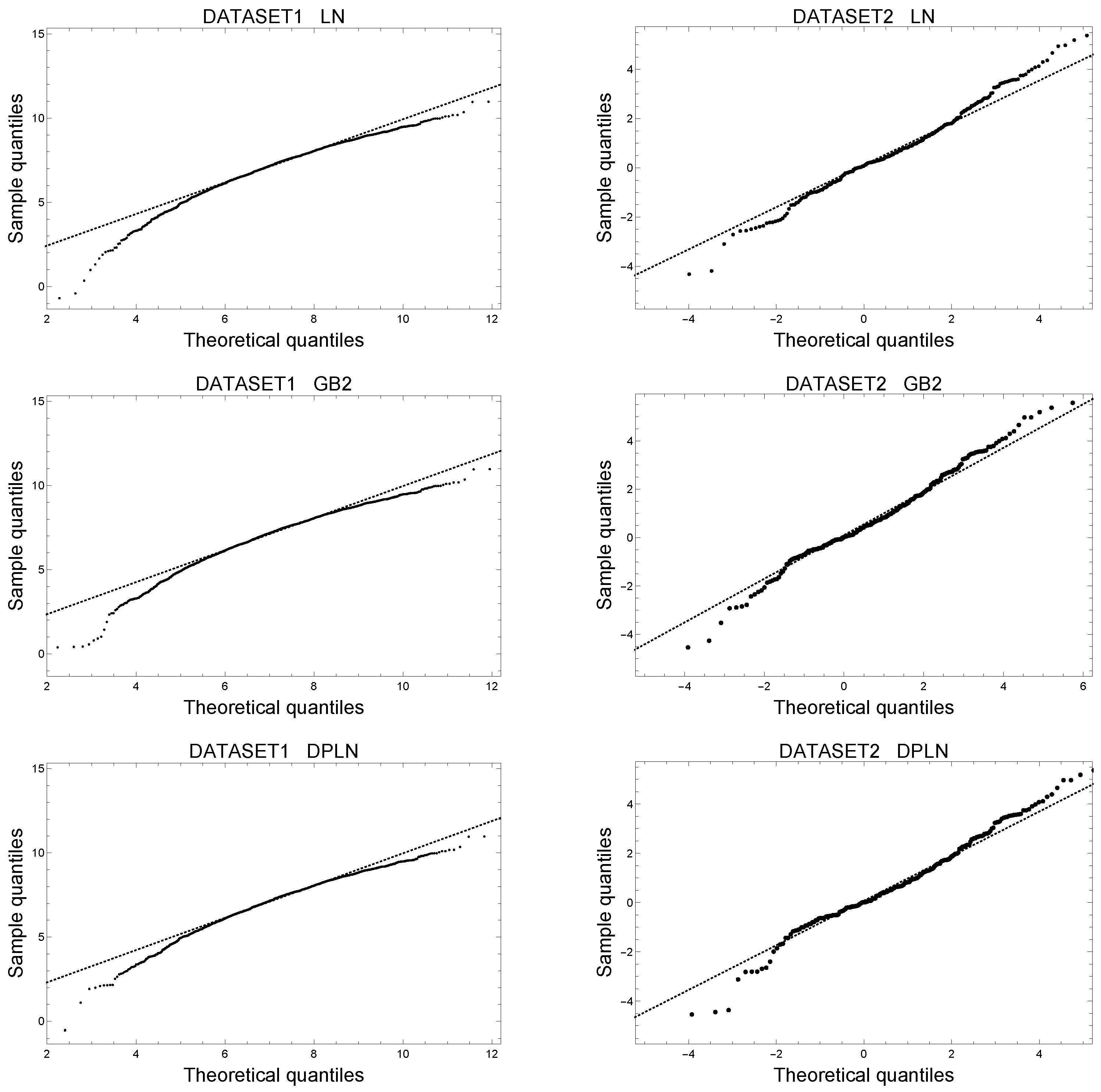
In the following we consider the log-residuals for assessing the goodness-of-fit of the proposed models for the two datasets considered. As the population moments of order higher than two cannot be derived neither for the DPLN (i.e., ${\lambda }_1<2$) nor the GB2 (i.e., the condition $p<2\tau <q$ is not satisfied in none of the datasets) distribution for the automobile bodily injury claims dataset, we have not examined the Pearson’s type residual. In Figure 2, one can see the QQ-plot of the log-residuals for LN, GB2 and DPLN generalized linear models for the automobile insurance claims (left hand side) automobile bodily injure claims data set (right hand side). The alignment along the 45-degree line is better in both the DPLN and GB2 generalized linear models in the central part and both tails of the distribution of the residuals as compared to the LN generalized linear model for the two datasets analyzed.

4.4. Out-of-Sample Validation of Models

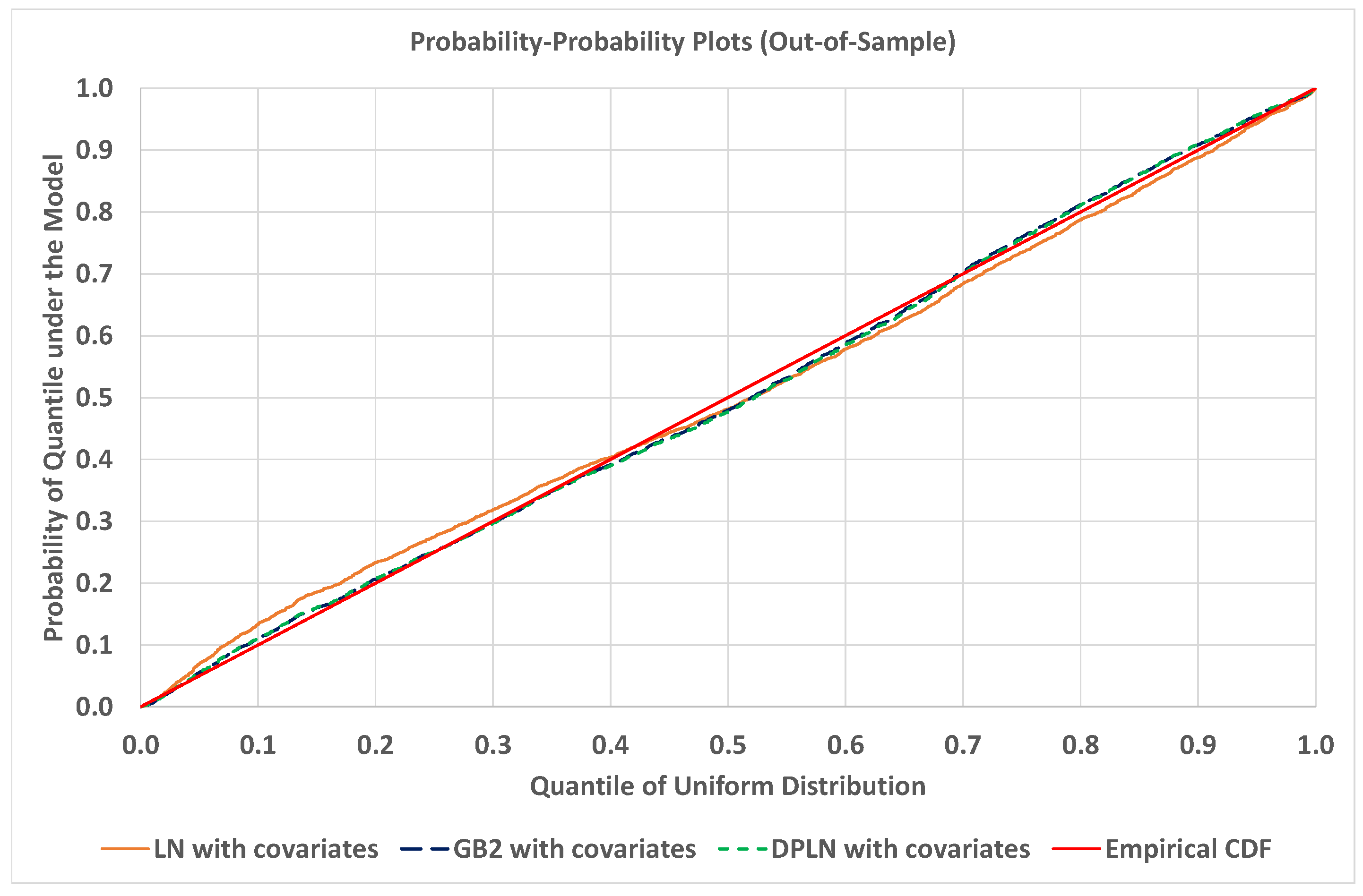
We demonstrate the abilities of the models to predict portfolio losses out-of-sample with probability-probability plots shown in Figure 3. The data set $\{v_1,v_2,\dots ,v_n\}$ is partitioned into two halves by sorting the claim sizes ascendingly, that is, we write the data set as

$$v_{i_1}<v_{i_2}<v_{i_3}<\dots <v_{i_n},$$

(33)

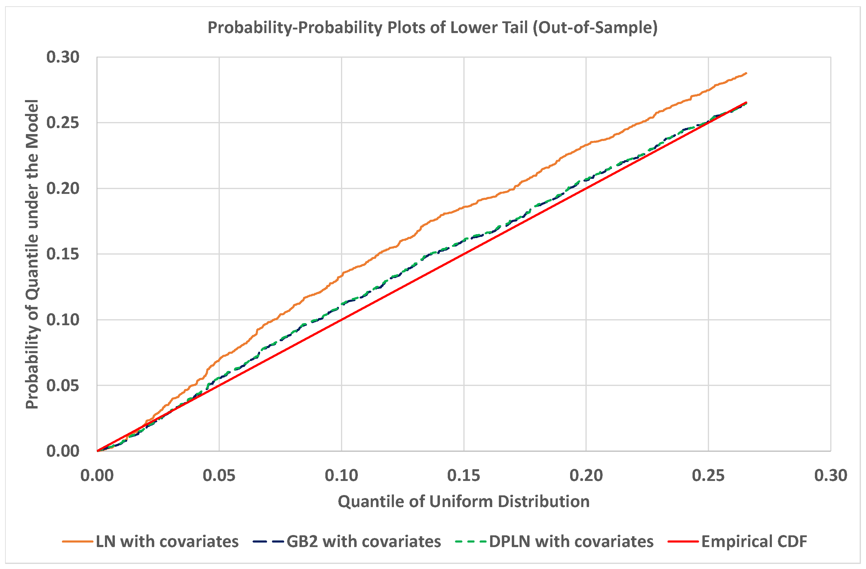
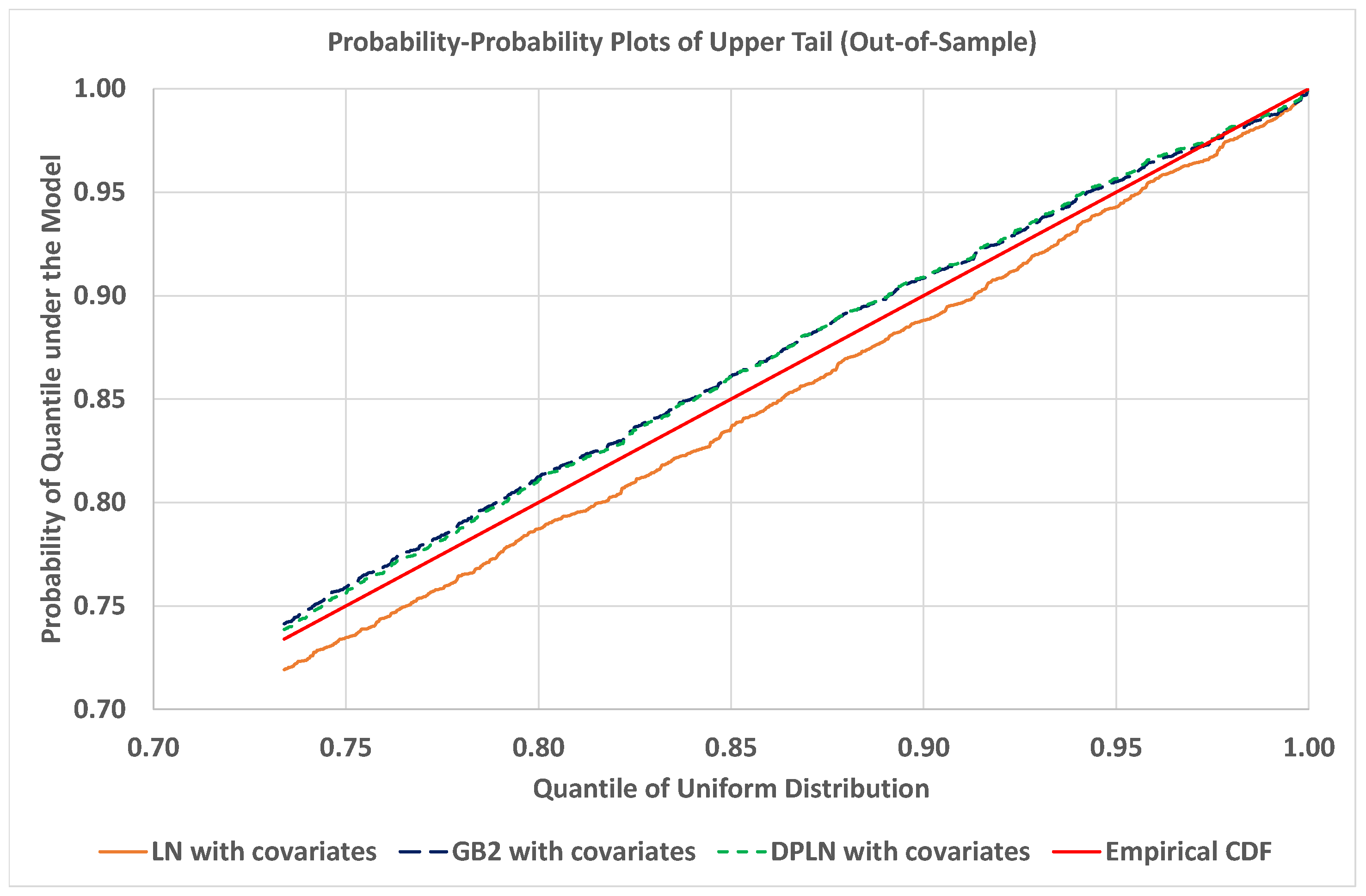
where $i_1,\dots ,i_n\in \{1,2,\dots ,n\}$, and then two data sets are formed, $A=\{v_{i_1},v_{i_3},v_{i_5},\dots \}$ and $B=\{v_{i_2},v_{i_4},v_{i_6},\dots \}$, alternating the data set to which each claim data item in the ordered data set is allocated. In this way the second data set is a good representation of the first data set in respect of claim distribution, but not necessarily in respect of the corresponding covariates, i.e., $\{{\mathit{x}}^{(i_2)},{\mathit{x}}^{(i_4)},\dots \}$ may not be representative of $\{{\mathit{x}}^{(i_1)},{\mathit{x}}^{(i_3)},\dots \}$. The data set A is used for fitting the models, whereas the data set B is used for graphing the probability-probability plots. In Figure 4 and Figure 5 we focus on the lower and upper tails of the distributions respectively, where it is evident that the DPLN and GB2 models provide the best fit and are almost indistiguishable.

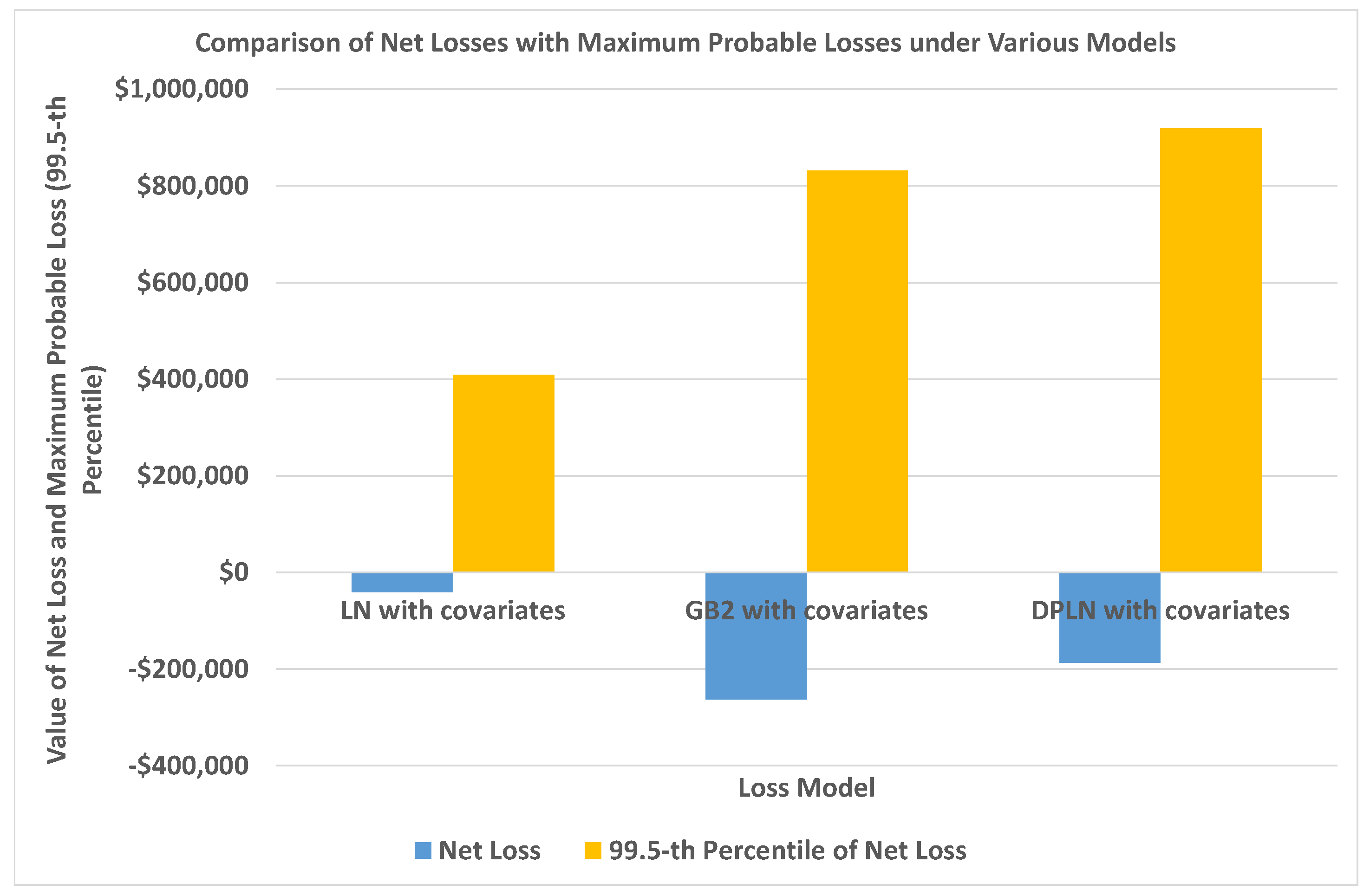
In Figure 6 the net losses under the various models are shown, where, as before, we have used half of the data for fitting the models and the other half for computing the net losses and maximum probable losses based on the 99.5-th percentile. It is evident that the DPLN and GB2 models give a higher computed maximum probable loss than for the LN distribution, and thus illustrates the ability of these models to provide adequate solvency levels when extreme claims are experienced by the insurer’s portfolio.

5. Conclusions

In this paper, the DPLN generalized linear model was developed and fitted to two data sets, these being private passenger automobile insurance claims data and automobile bodily injury claims data. Several covariates pertaining to various attributes of insurance claimants were combined in the linear predictor of the location parameter $\nu$, and were chosen because of their anticipated effect on claim size. This model exhibits Paretian behaviour in both tails and it is shown to provide fits to the two data sets which are comparable to those of the GB2 distribution.

The parameters of the DPLN generalized linear model were estimated via the EM algorithm and independently confirmed by maximizing the log-likelihood surface of the closely related Normal Laplace generalized linear model. The performance of the DPLN model has been compared with the lognormal distribution, a limiting case of the DPLN distribution, and the GB2 generalized linear model according to different model selection criteria. In view of the results obtained, we have found that the proposed DPLN generalized linear model is a valid alternative to other parametric heavy-tailed generalized linear models such as the GB2 GLM.

Potential practical applications of the DPLN GLM, beyond what is demonstrated in this article, include predicting mortality rates for lives where the covariates of the GLM are age, sex, occupation, etc. and predicting hazard rates in reduced-form credit risk models. These will be considered in further work.

References

1. Colombi, Roberto. 1990. A new model of income distribution: The Pareto lognormal distribution. In Income and Wealth Distribution, Inequality and Poverty. Edited by C. Dagum and M. Zenga. Berlin: Springer, pp. 18–32. [Google Scholar]
2. Dempster, Arthur P., Nan M. Laird, and Donald B. Rubin. 1977. Maximum likelihood estimation from incomplete data via the EM algorithm. Journal of the Royal Statistical Society Series B 39: 1–38. [Google Scholar]
3. Frees, Edward W., Richard A. Derrig, and Glenn Meyers. 2014a. Predictive Modeling Applications in Actuarial Science, Volume 1. New York: Cambridge University Press. [Google Scholar]
4. Frees, Edward W., Richard A. Derrig, and Glenn Meyers. 2014b. Predictive Modeling Applications in Actuarial Science, Volume 2. New York: Cambridge University Press. [Google Scholar]
5. Frees, Edward W., and Emiliano A. Valdez. 2008. Hierarchical Insurance Claims Modeling. Journal of the American Statistical Association 103: 1457–69. [Google Scholar] [CrossRef]
6. Giesen, Kristian, Arndt Zimmermann, and Jens Suedekum. 2010. The size distribution across all cities—Double Pareto lognormal strikes. Journal of Urban Economics 68: 129–37. [Google Scholar] [CrossRef]
7. Hajargasht, Gholamreza, and William E. Griffiths. 2013. Pareto-lognormal distributions: Inequality, poverty, and estimation from grouped income data. Economic Modelling 33: 593–604. [Google Scholar] [CrossRef]
8. Hürlimann, Werner. 2014. Pareto type distributions and excess-of-loss reinsurance. International Journal of Recent Research and Applied Studies 18: 1. [Google Scholar]
9. Kleiber, Christian, and Samuel Kotz. 2003. Statistical Size Distributions in Economics and Actuarial Sciences. Hoboken: Wiley. [Google Scholar]
10. Kočović, Jelena, Vesna Ćojbašić Rajić, and Milan Jovanović. 2015. Estimating a tail of the mixture of log-normal and inverse gaussian distribution. Scandinavian Actuarial Journal 2015: 49–58. [Google Scholar] [CrossRef]
11. Lehmann, Erich Leo, and George Casella. 1998. Theory of Point Estimation, 2nd ed. New York: Springer. [Google Scholar]
12. Louis, Thomas A. 1982. Finding the observed information matrix when using the EM algorithm. Journal of the Royal Statistical Society Series B 44: 226–33. [Google Scholar]
13. McDonald, James B. 1990. Regression model for positive random variables. Journal of Econometrics 43: 227–51. [Google Scholar] [CrossRef]
14. Ramirez-Cobo, Pepa, R. E. Lillo, S. Wilson, and M. P. Wiper. 2010. Bayesian inference for double pareto lognormal queues. The Annals of Applied Statistics 4: 1533–57. [Google Scholar] [CrossRef]
15. Reed, William J. 2003. The Pareto law of incomes - an explanation and an extension. Physica A 319: 469–86. [Google Scholar] [CrossRef]
16. Reed, William J., and Murray Jorgensen. 2004. The Double Pareto-Longnormal Distribution—A new parametric model for size distributions. Communications in Statistics - Theory and Methods 33: 1733–53. [Google Scholar] [CrossRef]
17. Vuong, Quang H. 1989. Likelihood ratio tests for model selection and non-nested hypotheses. Econometrica: Journal of the Econometric Society 57: 307–33. [Google Scholar] [CrossRef]
18. Wills, M., E. Valdez, and E. Frees. 2006. GB2 regression with insurance claim severities. Paper presented at the UNSW Actuarial Research Symposium, Sydney, New South Wales, Australia, November 9. [Google Scholar]
19. Yamaguchi, Kazuo. 1992. Accelerated failure-time regression models with a regression model of surviving fraction: An application to the analysis of ’permanent employment’ in Japan. Journal of the American Statistical Association 87: 284–92. [Google Scholar]
1.
Figure 1. Empirical distribution of the logarithm of automobile insurance claims (above) and logarithm of automobile bodily injury claims (below). The log transformation of the LN (N, black), DPLN (normal skew-Laplace (NSL), red) and GB2 ( L o g GB2, blue) distributions have been superimposed.
Risks 05 00060 g001
Figure 2. QQ-plots of the log-residuals for LN (above), GB2 (middle) and DPLN (below) generalized linear models for automobile insurance claims data (left panel) and automobile bodily injury claims (right panel).
Risks 05 00060 g002
Figure 3. Probability-probability plot (out-of-sample).
Risks 05 00060 g003
Figure 4. Probability-probability plot of lower tail (out-of-sample).
Risks 05 00060 g004
Figure 5. Probability-probability plots of upper tail (out-of-sample).
Risks 05 00060 g005
Figure 6. Net losses on a portfolio of automobile bodily injury claims for various models (out-of-sample).
Risks 05 00060 g006