Macroprudential Insurance Regulation: A Swiss Case Study

Abstract

This article provides a case study that analyzes national macroprudential insurance regulation in Switzerland. We consider an insurance market that is based on data from the Swiss private insurance industry. We stress this market with several scenarios related to financial and insurance risks, and we analyze the resulting risk capitals of the insurance companies. This stress-test analysis provides insights into the vulnerability of the Swiss private insurance sector to different risks and shocks.

1. Introduction

The insurance market is an important sector to the real economy. On the one hand, insurance companies provide financial services such as protection against financial losses and channeling savings into investments. On the other hand, they act as large investors supporting government, financial institutions and economy with capital. To ensure the proper functioning of the insurance industry, the companies are regulated by supervisory authorities. Their target is that each insurance company is able to meet its obligations towards its policyholders, even under adverse scenarios. For instance, in Switzerland private insurance companies are monitored by the Swiss Financial Market Supervisory Authority (FINMA). Its supervisory tool is the Swiss Solvency Test (SST) [1], which analyzes the balance sheet exposures and the solvability of an insurance company. This solvency test considers whether the risk capacity of the company is sufficient to run its business safely. Each Swiss private insurance company has to pass this SST on a stand-alone and annual basis.

Because of their similar underlying business, insurance companies invest into the same asset classes and they share the same liability classes. Consequently, the companies are exposed to the same risk factors so that adverse scenarios may disrupt these companies at the same time. This may imply that a large proportion of the companies cannot maintain their business, which may result in a severe shortage of the overall provided services. Therefore, it is of great importance that the insurance industry as a whole is resilient to adverse scenarios. This motivates us to consider the (Swiss) insurance market from a macroprudential perspective. This can be achieved by considering a network of insurers, where the companies are linked through common asset and liability classes. Moreover, these companies are linked through reinsurance agreements and through the holding of participations in other companies of the insurance market.

The structure of this insurance network is crucial for its vulnerability to financial shocks. One crucial characteristic of this structure is market concentration. A high market concentration may imply that the business of failed companies cannot be provided and maintained by other companies. Sources of high market concentration are the lack of competition, low price levels of premiums, and legal and regulatory constraints, see [2]. Figure 1 presents the market shares (based on earned premiums) of the three largest Swiss insurers for selected lines of business in year 2014. We observe rather high market concentration in many business lines.

Another crucial feature are investment and regulatory guidelines imposed by the supervisory authority. These guidelines may be reasonable for individual companies, but they may restrict asset portfolio choices too strongly so that several insurers have common investment strategies. These insurers are then exposed to very similar risks, and shocks may impact them simultaneously. This may also amplify the negative effects of their potential pro-cyclical behavior, see [2,4]. Figure 2 illustrates the asset allocations of 11 large Swiss life insurers by the end of year 2014. We observe that these insurers have very similar asset allocations.

For a more comprehensive overview of the risk drivers of an insurance market we refer to [2].

In this study we analyze the vulnerability of the Swiss insurance market as a whole to different risks, given its network structure. We introduce different stress scenarios and study their impact on the insurance network from a macroprudential point of view. The scenarios considered reflect two types of risks: financial market risks and insurance risks. Additionally, for these scenarios we study possible cascade effects arising from the network structure of the insurance market and from policyholder behavior. Such cascade effects are typically not considered in classical regulatory frameworks.

Besides classical financial risks, we also consider insurance risks that may impact the entire insurance industry, such as catastrophic events or changes in legislation. As an example for the latter, legal changes in the social security system may lead to a large number of (unexpected) disability claims for private companies offering accident insurance. Another example is that legislation and government in Switzerland decide on minimal financial guarantees and conversion rates in the pension system. This may heavily impact the life insurance sector, see the discussion on longevity in [5].

We define corresponding stress scenarios and investigate their impacts on the balance sheets of the insurance companies in Switzerland. This macroprudential analysis provides insights into the ability of the Swiss insurance market to absorb or to augment different risks and shocks.

Literature review. The macroprudential perspective is closely related to the concept of systemic risk; for an overview of the existing literature on systemic risk in insurance we refer to [6]. The latter reference analyzes the ability of the insurance industry to disrupt the financial market. It is indeed observed that insurers may contribute to the instability of the financial sector, especially through their noncore activities, see [7,8,9,10,11]. These observations are based on systemic risk measures that allow for the study of the interconnectedness between insurers and other financial institutions, see [12,13,14]. Such measures were also applied to parts of the European insurance industry, see [15]. Network analysis of the EU insurance sector is considered in [16], and its interconnectedness with the European banking sector analyzed in [17]. For further mathematical analysis of systemic risk in financial networks we refer to [18]. For a discussion on macroprudential regulatory frameworks we refer to [19,20,21].

In another stream of literature it is argued that a disruption of the insurance market does not have severe consequences to the financial sector, see [22,23,24,25]. In a similar spirit, [26] argues that the Swiss insurance market may not be systemic. Conversely, disruptions of the financial market may impact the insurance industry. Corresponding stress test analyses have been performed for some European countries, see for instance [27]. A stress test analyzing the wider European insurance market as a whole was performed by [28], see also [29]. The Swiss insurance market is not part of these studies. The present case study provides a stress test analysis of the Swiss insurance market by shocking this market with different scenarios. In contrast to the other studies, we also consider potential cascade effects resulting from these scenarios. Moreover, we explain in detail how the stress scenarios impact the balance sheet positions of a company, this also considers possible network effects. Additionally, to design the financial scenarios we consider market dependencies that are calibrated from historical data provided by FINMA [30]. This also allows us to back-test the scenarios and model calibration.

Outline of this paper. In the next section we formally introduce the market, in which we describe insurance companies and their balance sheets. Section 3 and Section 4 discuss the changes in the balance sheet positions when different risk factors are stressed. In Section 5 we provide a case study based on data from the Swiss private insurance market. We introduce an insurance market that has features similar to those of the Swiss market, see Section 5 for details. Then, we stress this market with different scenarios and analyze their impacts on the balance sheet positions of the insurance companies.

2. Insurance Market and Balance Sheet Structure

In this section we formally introduce the insurance market in which we study the impact of different risks. In Section 2.1 we describe insurance companies by their balance sheets and we link the companies through their investments and business. The different asset and liability classes are specified in more detail in Section 2.2.

2.1. Insurance and Financial Market

Denote by $I\in \mathbb{N}$ the number of insurance companies considered in the market. We assume that each insurer $i=1,\dots ,I$ can invest into $J\in \mathbb{N}$ different asset classes $a_j$, $j=1,\dots ,J$. Its liabilities can be allocated to $K\in \mathbb{N}$ different liability classes $l_k$, $k=1,\dots ,K$. The balance sheet of company i is denoted by ${\mathcal{V}}_i$ and is described by a vector

$${\mathcal{V}}_i=\left({\mathcal{V}}_i\left(a_1\right),\dots ,{\mathcal{V}}_i\left(a_J\right),{\mathcal{V}}_i\left(l_1\right),\dots ,{\mathcal{V}}_i\left(l_K\right),{\mathcal{V}}_i\left(r\right),{\mathcal{V}}_i\left(e\right)\right),$$

where the components are defined as follows:

• ${\mathcal{V}}_i\left(a_j\right)$ denotes the (market-consistent) value of company i’s investment into asset class $a_j$, $j=1,\dots ,J$.
• ${\mathcal{V}}_i\left(l_k\right)$ denotes the total liabilities of company i in liability class $l_k$, $k=1,\dots ,K$. This value is before (gross of) reinsurance.
• ${\mathcal{V}}_i\left(r\right)$ denotes the total reinsured part of the gross liabilities of company i. Hence, the net liabilities faced by company i is given by ${\sum }_{k=1}^K{\mathcal{V}}_i\left(l_k\right)-{\mathcal{V}}_i\left(r\right)$.
• ${\mathcal{V}}_i\left(e\right)={\sum }_{j=1}^J{\mathcal{V}}_i\left(a_j\right)-{\sum }_{k=1}^K{\mathcal{V}}_i\left(l_k\right)+{\mathcal{V}}_i\left(r\right)$ is the resulting own equity of company i that reflects its risk bearing capital.

We denote by $A_j$ the total market capitalization of asset class $a_j$ for $j=1,\dots ,J$. Note that

$$\sum _{i=1}^I{\mathcal{V}}_i\left(a_j\right)\le A_j,$$

because the insurance market shares asset class $a_j$ with other financial institutions. We may now think of the insurance market forming a network, since the insurers share the same asset and liability classes and they exchange reinsurance contracts. This implies that they are exposed to the same risk factors that link the insurance companies.

Additionally, asset classes themselves form a network with interacting asset classes. This second network will play the role of a feedback network to the insurance network. In particular, a relative change in total value $A_j$ of asset $a_j$ may also induce a change in total asset value $A_{j^{\prime }}$ of asset class $a_{j^{\prime }}$ for $j^{\prime }\ne j$ due to market dependencies. These changes may then influence ${\mathcal{V}}_i\left(a_j\right)$ and ${\mathcal{V}}_i\left(a_{j^{\prime }}\right)$ simultaneously, and potentially other items of the balance sheets ${\mathcal{V}}_i$. More details are given in Section 3 and Section 4.

2.2. Balance Sheet Structure

We structure the balance sheets ${\mathcal{V}}_i$ according to the Swiss Solvency Test (SST) guidelines, see for instance [30]. We choose Swiss franc (CHF) as the domestic currency and, for simplicity, we only consider euro (EUR) and U.S. dollar (USD) as foreign currencies. For term-dependent asset and liability classes we consider maturity buckets $t\in$ {1, 2, 3, 4, 5, 6, 7, 8, 9, 10, 15, 20, 30}; here, $t=10$ represents times to maturity of 10−12 years, $t=15$ represents 13−17 years, $t=20$ represents 18−24 years and $t=30$ represents times to maturity of at least 25 years. To simplify notation, we set

$$\begin{array}{ccc}\hfill \mathcal{T}& =& \{1,2,3,4,5,6,7,8,9,10,15,20,30\};\hfill \\ \hfill \mathcal{C}& =& \{\mathrm{CHF},\mathrm{EUR},\mathrm{USD}\};\hfill \\ \hfill \mathcal{R}& =& \{\mathrm{RF},\mathrm{AAA},\mathrm{AA},\mathrm{A},\mathrm{BBB},\mathrm{BB}\},\hfill \end{array}$$

where $\mathcal{R}$ lists credit ratings for term-dependent assets. Rating RF corresponds to risk-free assets. These we define to be term-dependent assets whose valuations do not consider any credit spread, see next paragraph. We use this balance sheet structure for our analysis, but it can easily be extended.

Table 1. Asset and liability classes under consideration, including their notation. The upper indexes run over maturity buckets $t\in \mathcal{T}$, currencies $w\in \mathcal{C}$ and ratings $r\in \mathcal{R}$, respectively.

Asset Classes ${\mathit{a}}_{\mathit{j}}$		Liability Classes ${\mathit{l}}_{\mathit{k}}$
real estate:		insurance provisions for
− residential real estate	$a_{\mathrm{re},\mathrm{r}}$	− collective life insurance:
− commercial real estate	$a_{\mathrm{re},\mathrm{c}}$	occupational benefits insurance	$l_{\mathrm{ob}}^t$
participations in		− individual life insurance:
− other network participants	$a_{\mathrm{part},\mathrm{ins}}^w$	endowment insurance	$l_{\mathrm{ei}}^t$
− real estate related firms	$a_{\mathrm{part},\mathrm{re}}^w$	pension annuities	$l_{\mathrm{pa}}^t$
− others	$a_{\mathrm{part},\mathrm{o}}^w$	unit-linked life insurance	$l_{\mathrm{ul}}$
fixed-income securities	$a_{\mathrm{bonds}}^{w,t,r}$	other individual life insurance	$l_{\mathrm{oli}}^t$
loans	$a_{\mathrm{loans}}^{w,t,r}$	− non-life insurance:
mortgages	$a_{\mathrm{mortgages}}^{w,t,r}$	accident insurance	$l_{\mathrm{ai}}^t$
equity	$a_{\mathrm{equity}}^w$	health insurance	$l_{\mathrm{hi}}^t$
collective investments in		motor insurance	$l_{\mathrm{mi}}^t$
− real estate funds	$a_{\mathrm{ci},\mathrm{ref}}$	property insurance	$l_{\mathrm{pi}}^t$
− equity investment funds	$a_{\mathrm{ci},\mathrm{ef}}$	casualty insurance	$l_{\mathrm{ci}}^t$
− others	$a_{\mathrm{ci},\mathrm{o}}$	other non-life insurance	$l_{\mathrm{onli}}^t$
alternative investments in		− business abroad	$l_{\mathrm{ba}}^{w,t}$
− hedge funds	$a_{\mathrm{ai},\mathrm{hf}}$	− backing cover	$l_{\mathrm{bc}}^t$
− private equity	$a_{\mathrm{ai},\mathrm{pe}}$	liabilities from insurance and
− others	$a_{\mathrm{ai},\mathrm{o}}$	investment activities	$l_{\mathrm{la}}$
investments from unit-linked life insurance	$a_{\mathrm{ul}}$	other liabilities	$l_{\mathrm{o}}$
cash and other assets	$a_{\mathrm{cash}}^w$, $a_{\mathrm{o}}$

lists the asset classes considered. We consider term-dependent assets, i.e. fixed-income securities, loans and mortgages, for different maturities $t\in \mathcal{T}$, ratings $r\in \mathcal{R}$ and currencies $w\in \mathcal{C}$ as separate asset classes. By the SST guidelines, real estate is considered to be term-independent. We assume that only government bonds with currencies CHF and USD are considered to be risk-free assets, and that mortgages have rating $\mathrm{A}\in \mathcal{R}$. This is in line with the SST guidelines, see [31]. However, we include all ratings to every term-dependent asset in order to have a consistent notation. If there is not a currency explicitly mentioned, the underlying currency is assumed to be CHF.

Table 1 also lists the liability classes considered. Typically, the largest liability class of an insurer consists of its insurance provisions (reserves) for different lines of business. For each line of business we consider the provisions for different expected maturity dates $t\in \mathcal{T}$ separately. Note that, except for business abroad, the underlying currency is assumed to be CHF. This is because we aim at studying the local business. Below, we may further categorize some lines of business because of the different structures of their payment patterns. For example, for accident insurance we distinguish between insurance provisions for annuities and for short/long-term liabilities.

3. Risk Factors and Their Impact on the Market

In the previous section we have introduced the insurers’ balance sheets ${\mathcal{V}}_i$ and the financial market. We will shock these by stressing risk factors which we categorize into two groups: in Section 3.1 we consider financial market risk factors, and in Section 3.2 we consider other risk factors that do not directly impact the total market capitalizations, such as biometric risks and risks arising from policyholder behavior.

We denote the risk-free zero-coupon rates by $r_{w,t}$ for currency $w\in \mathcal{C}$ and maturity bucket $t\in \mathcal{T}$. The credit spreads are denoted by $s_{w,r}$ for currency $w\in \mathcal{C}$ and rating $r\in \mathcal{R}$. Here, the spreads for a given currency and a given rating are assumed to be constant over different maturities. Recall that rating $\mathrm{RF}\in \mathcal{R}$ corresponds to term-dependent assets where no credit spread is added to the risk-free rates. Therefore, we set $s_{w,\mathrm{RF}}=0$ for all $w\in \mathcal{C}$, throughout.

3.1. Market Risk Factors

We consider the market risk factors listed in

Table 2. Market risk factors considered, including the notation for their changes. The lower indexes run over maturity buckets $t\in \mathcal{T}$, currencies $w\in \mathcal{C}$ and ratings $r\in \mathcal{R}$, respectively.

Market Risk Factors
zero-coupon rates	$\mathrm{\Delta }{Z}_{w,t}^{\mathrm{zeros}}$
credit spreads	$\mathrm{\Delta }{Z}_{w,r}^{\mathrm{spreads}}$
exchange rates	$\mathrm{\Delta }{Z}_w^{\mathrm{FX}}$
equity	$\mathrm{\Delta }{Z}_w^{\mathrm{equity}}$
hedge funds, private equity and real estate funds	$\mathrm{\Delta }{Z}^{\mathrm{hf}}$, $\mathrm{\Delta }{Z}^{\mathrm{pe}}$, $\mathrm{\Delta }{Z}^{\mathrm{ref}}$
residential real estate and commercial real estate	$\mathrm{\Delta }{Z}^{\mathrm{re},\mathrm{r}}$, $\mathrm{\Delta }{Z}^{\mathrm{re},\mathrm{c}}$
participations	$\mathrm{\Delta }{Z}^{\mathrm{part}}$

, their changes are denoted by $\mathrm{\Delta }Z$. The changes in zero-coupon rates and credit spreads are assumed to be absolute changes. The changes in the remaining market risk factors are considered to be relative changes. As an example, a change $\mathrm{\Delta }{Z}_{\mathrm{EUR}}^{\mathrm{FX}}$ implies a new exchange rate EUR/CHF given by $1+\mathrm{\Delta }{Z}_{\mathrm{EUR}}^{\mathrm{FX}}$ times the previous rate. We set $\mathrm{\Delta }{Z}_{\mathrm{CHF}}^{\mathrm{FX}}=0$ and $\mathrm{\Delta }{Z}_{w,\mathrm{RF}}^{\mathrm{spreads}}=0$ for each $w\in \mathcal{C}$, throughout. Shocking risk factors will result in $\mathrm{\Delta }Z$ being different from 0.

Changes in market risk factors affect the total market capitalizations of the asset classes listed in Table 1. In turn, these changes impact each insurer’s balance sheet. This is explained next.

Fixed-income securities, loans and mortgages. The relative change in the total market capitalization of fixed-income securities with underlying currency $w\in \mathcal{C}$, maturity date $t\in \mathcal{T}$ and rating $r\in \mathcal{R}$ is given by

$$\frac{\mathrm{\Delta }{A}_{\mathrm{bonds}}^{w,t,r}}{A_{\mathrm{bonds}}^{w,t,r}}=\left(1+\mathrm{\Delta }{Z}_w^{\mathrm{FX}}\right){\left(1+\frac{\mathrm{\Delta }{Z}_{w,t}^{\mathrm{zeros}}+\mathrm{\Delta }{Z}_{w,r}^{\mathrm{spreads}}}{1+r_{w,t}+s_{w,r}}\right)}^{-t}-1.$$

Similarly for loans and mortgages.

Equity and equity investment funds. The relative changes in total market capitalizations of equity for currency $w\in \mathcal{C}$ and of equity investment funds are given by

$$\frac{\mathrm{\Delta }{A}_{\mathrm{equity}}^w}{A_{\mathrm{equity}}^w}=\left(1+\mathrm{\Delta }{Z}_w^{\mathrm{FX}}\right)\left(1+\mathrm{\Delta }{Z}_w^{\mathrm{equity}}\right)-1\mathrm{and}\frac{\mathrm{\Delta }{A}_{\mathrm{ci},\mathrm{ef}}}{A_{\mathrm{ci},\mathrm{ef}}}=\mathrm{\Delta }{Z}_{\mathrm{CHF}}^{\mathrm{equity}},$$

respectively.

Participations. The relative change in market capitalization of participations in real estate related firms is modeled by

$$\frac{\mathrm{\Delta }{A}_{\mathrm{part},\mathrm{re}}^w}{A_{\mathrm{part},\mathrm{re}}^w}=\left(1+\mathrm{\Delta }{Z}_w^{\mathrm{FX}}\right)\left(1+\frac{\mathrm{\Delta }{Z}^{\mathrm{re},\mathrm{r}}+\mathrm{\Delta }{Z}^{\mathrm{re},\mathrm{c}}}{2}\right)-1,$$

for $w\in \mathcal{C}$. The relative change in total market capitalization of participations in other firms, except other network participants, is given by

$$\frac{\mathrm{\Delta }{A}_{\mathrm{part},\mathrm{o}}^w}{A_{\mathrm{part},\mathrm{o}}^w}=\left(1+\mathrm{\Delta }{Z}_w^{\mathrm{FX}}\right)\left(1+\mathrm{\Delta }{Z}^{\mathrm{part}}\right)-1,$$

for $w\in \mathcal{C}$.

Remark 1.

Observe that a company $i=1,\dots ,I$ of the insurance market may hold participations in other network participants, its total investment is denoted by ${\mathcal{V}}_i\left(a_{part,ins}^w\right)$. The change in value of an investment in network participant $i^{\prime }\ne i$ is dependent on the risk bearing capital of company $i^{\prime }$. This will be modeled more explicitly in Section 4.

Other asset classes. The market capitalizations of the asset classes in {hedge funds, private equity, real estate funds, residential real estate, commercial real estate, cash} are influenced by the market risk factors in Table 2 in the intuitive way. For simplicity, we assume that the asset classes $a_{\mathrm{ci},\mathrm{o}}$, $a_{\mathrm{ai},\mathrm{o}}$ and $a_{\mathrm{o}}$ are not influenced by changes in market risk factors. Due to the strong linkage of a company’s investments from unit-linked life insurance to its corresponding insurance provisions we assume that changes in these two positions are equal. Hence, a change in value of these investments does not affect the insurer’s risk bearing capital. As such, we forgo modeling impacts on asset class $a_{\mathrm{ul}}$ due to changes in the market risk factors.

The changes in total market capitalizations described above directly impact the value of each insurer’s investments. The relative change in value of company i’s investment into asset class $a_j$ is modeled by

$$\frac{\mathrm{\Delta }{\mathcal{V}}_i\left(a_j\right)}{{\mathcal{V}}_i\left(a_j\right)}=\frac{\mathrm{\Delta }{A}_j}{A_j},$$

for each asset class $a_j$ listed in Table 1 and each insurer $i=1,\dots ,I$.

Changes in market risk factors also impact the liability side of an insurer’s balance sheet. For simplicity, we assume that the market risk factors only affect the insurance provisions, see Table 1. Note that these typically form the largest position on the liability side. Recall that ${\mathcal{V}}_i\left(l_k^t\right)$ denotes company i’s gross value of the outstanding liabilities with expected maturity date $t\in \mathcal{T}$ for line of business $l_k$. The relative change in this value is given by

$$\frac{\mathrm{\Delta }{\mathcal{V}}_i\left(l_k^t\right)}{{\mathcal{V}}_i\left(l_k^t\right)}={\left(1+\frac{\mathrm{\Delta }{Z}_{\mathrm{CHF},t}^{\mathrm{zeros}}}{1+r_{\mathrm{CHF},t}}\right)}^{-t}-1,$$

for each line of business $l_k$ listed in Table 1 (except business abroad and unit-linked life insurance) and each $t\in \mathcal{T}$. Similarly for business abroad and for the relative change in reinsured liabilities.

Finally, the relative change in the own equity ${\mathcal{V}}_i\left(e\right)$ of insurer $i=1,\dots ,I$ is given by

$$\frac{\mathrm{\Delta }{\mathcal{V}}_i\left(e\right)}{{\mathcal{V}}_i\left(e\right)}=\frac{1}{{\mathcal{V}}_i\left(e\right)}\left(\sum _j{\mathcal{V}}_i\left(a_j\right)\frac{\mathrm{\Delta }{A}_j}{A_j}-\sum _k\mathrm{\Delta }{\mathcal{V}}_i\left(l_k\right)+\mathrm{\Delta }{\mathcal{V}}_i\left(r\right)\right).$$

Remark 2.

For the case study provided in Section 5 we approximate the changes in the market risk factors listed in Table 2, except $\mathrm{\Delta }{Z}^{ref}$ and $\mathrm{\Delta }{Z}^{part}$, by a multivariate normal distribution with mean vector being the null vector and a predefined positive definite covariance matrix. This is in line with the SST guidelines, see [31], and allows us to model market dependencies. In fact, the only property of this approximation we explicitly need in our analysis is the following: conditionally given fixed changes in selected market risk factors, the conditional changes in the remaining risk factors have again a multivariate normal distribution with mean vector and covariance matrix given by Lemma 1, below, see for instance [32]. We emphasize that the tail of the normal distribution is not used, because we will stress-test selected risk classes and analyze the conditionally expected influence on the remaining risk classes. More precisely, for the case study in Section 5 we consider stress scenarios defined as follows: we predefine changes $\mathrm{\Delta }{\mathit{Z}}_1=\mathrm{\Delta }{\mathit{z}}_1$ in selected market risk factors and, given these changes, we consider the conditionally expected changes $\mathrm{\Delta }{\mu }_{2|1}$ in the remaining components according to Lemma 1. We set $\mathrm{\Delta }{Z}^{ref}=\mathrm{\Delta }{Z}^{ref,c}$ and $\mathrm{\Delta }{Z}^{part}=\mathrm{\Delta }{Z}_{CHF}^{equity}$. We will illustrate this in the figures in Section 5.1 by showing the predefined risk factor changes $\mathrm{\Delta }{\mathit{Z}}_1=\mathrm{\Delta }{\mathit{z}}_1$ in green color and the conditionally expected changes $\mathrm{\Delta }{\mu }_{2|1}$ in the other risk factors in orange color. Given these changes in the risk factors, we update the market capitalization of each asset and the balance sheet of each company accordingly, as described above.

Lemma 1.

Fix $d\ge 1$. Let $\mathit{Y}={(Y_1,\dots ,Y_d)}^{\prime }$ have a multivariate normal distribution with mean vector $\mathbf{\mu }\in {\mathbb{R}}^d$ and positive definite covariance matrix $\Sigma \in {\mathbb{R}}^{d\times d}$. Let $1\le k<d$ and write $\mathit{Y}={({\mathit{Y}}_1^{\prime },{\mathit{Y}}_2^{\prime })}^{\prime }$ with ${\mathit{Y}}_1={(Y_1,\dots ,Y_k)}^{\prime }$ and ${\mathit{Y}}_2={(Y_{k+1},\dots ,Y_d)}^{\prime }$. Accordingly, we write

$$\mathbf{\mu }={({\mathbf{\mu }}_1^{\prime },{\mathbf{\mu }}_2^{\prime })}^{\prime }\mathrm{and}\Sigma =\left(\begin{array}{cc}{\Sigma }_{11}& {\Sigma }_{12}\\ {\Sigma }_{21}& {\Sigma }_{22}\end{array}\right),$$

with ${\Sigma }_{11}\in {\mathbb{R}}^{k\times k}$, ${\Sigma }_{12}={\Sigma }_{21}^{\prime }\in {\mathbb{R}}^{k\times (d-k)}$ and ${\Sigma }_{22}\in {\mathbb{R}}^{(d-k)\times (d-k)}$. Then, the conditional distribution of ${\mathit{Y}}_2$, given ${\mathit{Y}}_1={\mathit{y}}_1$, is again a multivariate normal distribution with mean vector ${\mathbf{\mu }}_{2|1}\in {\mathbb{R}}^{d-k}$ and positive definite covariance matrix ${\Sigma }_{22|1}\in {\mathbb{R}}^{(d-k)\times (d-k)}$ given by

$${\mathbf{\mu }}_{2|1}={\mathbf{\mu }}_2+{\Sigma }_{21}{\Sigma }_{11}^{-1}\left({\mathit{y}}_1-{\mathbf{\mu }}_1\right)\mathrm{and}{\Sigma }_{22|1}={\Sigma }_{22}-{\Sigma }_{21}{\Sigma }_{11}^{-1}{\Sigma }_{12}.$$

Thus, ${\mathbf{\mu }}_{2|1}$ describes the conditionally expected outcome in ${\mathit{Y}}_2$, given ${\mathit{Y}}_1={\mathit{y}}_1$.

3.2. Further Risk Factors and Cascade Effects

For the case study in Section 5 we consider further risks that do not directly impact the total market capitalization. Examples are biometric risks and risks arising from policyholder behavior. In this section we discuss some of these risks and their impact on the balance sheets. Note that some of these risks may arise as cascade effects triggered by changes in the market risk factors as discussed in Section 3.1.

Longevity risk. We only consider longevity risk for life and accident insurance. Let $q_{x,0}\in [0,1]$ be the probability of a policyholder with age $x\in \mathbb{N}$ to die within the current accounting year $(t=0)$. Denote by $q_{x,t}$ the probability of a policyholder who is aged $x\in \mathbb{N}$ in accounting year $t\ge 1$ to die within that accounting year t. We assume that $q_{x,t}$, $x,t\in \mathbb{N}$, is of the form

$$q_{x,t}=q_{x,0}{e}^{-{\lambda }_{x,t}},$$

for some ${\lambda }_{x,t}>0$. We model longevity risk by considering a relative change in ${\lambda }_{x,t}$, denoted by $\mathrm{\Delta }{Z}^{\lambda }>0$, for all $x\ge 65$ and $t\ge 1$. The resulting mortality rates are then given by

$${\tilde{q}}_{x,t}=q_{x,0}{e}^{-(1+\mathrm{\Delta }{Z}^{\lambda }){\lambda }_{x,t}}=q_{x,t}{e}^{-\mathrm{\Delta }{Z}^{\lambda }{\lambda }_{x,t}},$$

(1)

for $x\ge 65$ and $t\ge 1$, and ${\tilde{q}}_{x,t}=q_{x,t}$, else. The absolute change in insurance provisions resulting from the new mortality rates is given by the difference between the insurance provisions calculated using the new mortality rates ${\tilde{q}}_{x,t}$ and the insurance provisions calculated using the initial rates $q_{x,t}$.

Decline in new business. We consider a financial loss that arises due to planned but unearned future premium in new business. This assumes that administrative expenses of a company are non-linear in the earned premium on a short time scale. The unexpected relative change in new business is denoted by $\mathrm{\Delta }{Z}^{\mathrm{nb}}<0$. We model the resulting absolute loss in cash of firm $i=1,\dots ,I$ by

$$-\mathrm{\Delta }{Z}^{\mathrm{nb}}{c}_i{\mathcal{V}}_i\left(p^{\mathrm{nb}}\right).$$

Here, $c_i\in [0,1]$ denotes the cost ratio of company i and ${\mathcal{V}}_i\left(p^{\mathrm{nb}}\right)$ denotes its expected earned premium in new business for the coming accounting year.

Lapse risk. We consider lapse risk only for individual life insurance. Lapse risk could also be considered in occupational benefit insurance (and in other lines of business). However, in contrast to individual life insurance, surrendered portfolios need to be transferred to other insurance companies or pension funds, including the investments. Therefore, the impact on the market as a whole presumably stays small. For this reason we only consider surrenders in individual life insurance, namely in unit-linked and endowment insurance. We denote the absolute change in the expected lapse rate by $\mathrm{\Delta }{Z}^{\mathrm{lapse}}>0$.

The relative changes in investments and insurance provisions for unit-linked life insurance of firm $i=1,\dots ,I$ due to the unexpected surrenders are assumed to be equal. We model these changes by

$$\frac{\mathrm{\Delta }{\mathcal{V}}_i\left(a_{\mathrm{ul}}\right)}{{\mathcal{V}}_i\left(a_{\mathrm{ul}}\right)}=\frac{\mathrm{\Delta }{\mathcal{V}}_i\left(l_{\mathrm{ul}}\right)}{{\mathcal{V}}_i\left(l_{\mathrm{ul}}\right)}=-\mathrm{\Delta }{Z}^{\mathrm{lapse}}.$$

Here, we assume that the aggregated surrender value equals $\mathrm{\Delta }{\mathcal{V}}_i\left(a_{\mathrm{ul}}\right)=\mathrm{\Delta }{\mathcal{V}}_i\left(l_{\mathrm{ul}}\right)$ and is raised by selling the underlying investments. However, note that asset prices are typically stressed if lapse rates are unexpectedly high. Therefore, we assume that the investments $\mathrm{\Delta }{\mathcal{V}}_i\left(a_{\mathrm{ul}}\right)$ can only be sold at a price which is ℓ times the booked value, for some $\ell \in (0,1]$. The remaining part $(1-\ell )\mathrm{\Delta }{\mathcal{V}}_i\left(a_{\mathrm{ul}}\right)$ of the aggregated surrender value is then, for example, raised by cash.

For endowment insurance, typically only policies with a savings part can be lapsed. For company $i=1,\dots ,I$, we denote by ${\mathcal{V}}_i\left(l_{\mathrm{ei},\mathrm{m}}\right)$ its insurance provisions for these policies. We denote by ${\mathcal{V}}_i\left(l_{\mathrm{ei},\mathrm{m}}\left(s\right)\right)$ the insurance provisions for such policies with a remaining duration of $s\in \mathbb{N}$ years, note that ${\sum }_s{\mathcal{V}}_i\left(l_{\mathrm{ei},\mathrm{m}}\left(s\right)\right)={\mathcal{V}}_i\left(l_{\mathrm{ei},\mathrm{m}}\right)\le {\mathcal{V}}_i\left(l_{\mathrm{ei}}\right)$. Among all unexpected surrendered policies, let $m_s\in [0,1)$ be the proportion of lapsed policies with a remaining duration of $s\in \mathbb{N}$ years, observe ${\sum }_s{m}_s=1$. Factors $m_s$ will be used to model policyholders’ surrender behavior which typically depends on the remaining duration of the individual contract. We model the relative change in insurance provisions for endowment insurance due to the unexpected surrenders by

$$\frac{\mathrm{\Delta }{\mathcal{V}}_i\left(l_{\mathrm{el},\mathrm{m}}\right)}{{\mathcal{V}}_i\left(l_{\mathrm{el},\mathrm{m}}\right)}=-\mathrm{\Delta }{Z}^{\mathrm{lapse}}\frac{{\sum }_s{m}_s{\mathcal{V}}_i\left(l_{\mathrm{ei},\mathrm{m}}\left(s\right)\right)}{{\mathcal{V}}_i\left(l_{\mathrm{el},\mathrm{m}}\right)}.$$

For company $i=1,\dots ,I$, denote by ${\mathcal{S}}_i\left(l_{\mathrm{ei},\mathrm{m}}\left(s\right)\right)$ the total surrender value if all its policies (with a savings part) with a remaining duration of $s\in \mathbb{N}$ years were lapsed. The total amount insurer i has to pay to the surrendered policyholders is assumed to be

$$\mathrm{\Delta }{Z}^{\mathrm{lapse}}\sum _s{m}_s{\mathcal{S}}_i\left(l_{\mathrm{ei},\mathrm{m}}\left(s\right)\right).$$

(2)

We assume that this amount is raised by cash or by selling investments. We further assume that these investments can only be sold at a price which is ℓ times the booked value, for some $\ell \in (0,1]$. Again, factor ℓ will be used to stress asset prices.

Lapsed policies further imply losses due to the absence of corresponding planned future premium. These losses are modeled similarly as for a decline in new business.

Other risks. Further risks such as underreserving, catastrophic events or a failure of reinsurers are discussed in the case study, see Section 5.

Remark 3.

If an insurer $i=1,\dots ,I$ runs out of cash, i.e. ${\mathcal{V}}_i\left(a_{cash}^w\right)<0$ for all $w\in \mathcal{C}$, we assume that it generates amount $-{\sum }_{w\in \mathcal{C}}{\mathcal{V}}_i\left(a_{cash}^w\right)$ by selling investments. Again, we assume that all these investments can only be sold at a price which is ℓ times the corresponding value in the balance sheet, for some $\ell \in (0,1]$.

4. Network Effects Followed from Changes in Risk Factors

In Section 3 we have studied risk factors and their impacts on the balance sheets of the insurers. These impacts may lead to further cascade effects. This is because of market dependencies and the network structure of the insurance market. In the following we discuss some of these effects that we consider for the case study in Section 5.

Market impact due to the sale of assets. We assume that the sale of an asset in large amounts changes its price. This, in turn, impacts each insurer investing in this asset class. Let $S_j$ be the total value of asset $a_j$ sold by all the insurers, for instance, due to unexpected lapses or a liquidity shortage. We model the relative change in the total market capitalization of asset $a_j$ triggered by the sales of this asset by

$$\frac{\mathrm{\Delta }{A}_j}{A_j}=p_j=e^{-\alpha S_j/A_j}-1,\mathrm{with}\alpha >0.$$

(3)

Here, $A_j$ denotes the total market capitalization of asset $a_j$ (which may have changed due to changes in market risk factors), and the second equality defines the price impact $p_j$. We choose α such that $e^{-\alpha /10}=0.9$. This choice implies a $10\%$ drop in total market capitalization when $10\%$ of the corresponding assets were sold, and is supported by [33].

These price impacts further affect the market capitalization of other assets due to market dependencies. Since we study a local market with domestic currency CHF, we only focus on assets with this underlying currency. We model their dependencies through the market risk factors listed in

Table 3. Market risk factors considered for modeling the market impact caused by the sale of assets in large amounts.

Market Risk Factors
CHF zero-coupon rates for maturities $t\in \mathcal{T}$	$\mathrm{\Delta }{Z}_{\mathrm{CHF},t}^{\mathrm{zeros}}$
CHF credit spreads for ratings $r\in \mathcal{R}\backslash \left\{\mathrm{RF}\right\}$	$\mathrm{\Delta }{Z}_{\mathrm{CHF},r}^{\mathrm{spreads}}$
equity for currency CHF	$\mathrm{\Delta }{Z}_{\mathrm{CHF}}^{\mathrm{equity}}$
hedge funds, private equity and real estate funds	$\mathrm{\Delta }{Z}^{\mathrm{hf}}$, $\mathrm{\Delta }{Z}^{\mathrm{pe}}$, $\mathrm{\Delta }{Z}^{\mathrm{ref}}$
residential real estate and commercial real estate	$\mathrm{\Delta }{Z}^{\mathrm{re},\mathrm{r}}$, $\mathrm{\Delta }{Z}^{\mathrm{re},\mathrm{c}}$

in the following way. For example, consider asset class $a_{\mathrm{equity}}^{\mathrm{CHF}}$ and assume a nonzero price impact $p_{\mathrm{equity}}^{\mathrm{CHF}}$. Note that this price impact changes the total market capitalization of $a_{\mathrm{equity}}^{\mathrm{CHF}}$ as if we would set $\mathrm{\Delta }{Z}_{\mathrm{CHF}}^{\mathrm{equity}}=p_{\mathrm{equity}}^{\mathrm{CHF}}$, see Section 3.1. Then, under the assumptions of Remark 2, the conditionally expected changes in the remaining risk factors in Table 3, except $\mathrm{\Delta }{Z}^{\mathrm{ref}}$, are again given by Lemma 1. We will illustrate this in the figures below, see Section 5.2, by showing the risk factor changes $\mathrm{\Delta }{\mathit{Z}}_1=\mathrm{\Delta }{\mathit{z}}_1$ given by the price impact in green color, and the conditionally expected changes $\mathrm{\Delta }{\mathbf{\mu }}_{2|1}$ in the other risk factors due to market dependencies in orange color. Given these changes in the risk factors, we update the market capitalization of each asset and the balance sheet of each company as described in Section 3.1.

Remark 4.

If we consider a nonzero price impact of a term-dependent asset, say, $p_{bonds}^{CHF,t}$ for fixed-income securities with currency CHF and maturity $t\in \mathcal{T}$, we represent this price impact by setting

$$\mathrm{\Delta }{Z}_{CHF,t}^{zeros}=\left(1+r_{CHF,t}\right)\left({\left(p_{bonds}^{CHF,t}+1\right)}^{-1/t}-1\right).$$

The conditionally expected changes in the remaining risk factors listed in Table 3 are then defined as above using Lemma 1. Observe that $\mathrm{\Delta }{Z}_{zeros}^{CHF,t}$ as defined above does not exactly imply changes in market capitalizations $A_{bonds}^{CHF,t,r}$ given by (3) for every rating $r\in \mathcal{R}$. This is because in $\mathrm{\Delta }{Z}_{CHF,t}^{zeros}$ above we have ignored any credit spread.

Reinsurance. We do not consider any explicit links between primary insurers and reinsurers within the insurance network (except potential participations, see below). In particular, we do not specify which reinsurers take over the reinsured liabilities ${\mathcal{V}}_i\left(r\right)$ of firm $i=1,\dots ,I$; note that reinsurance business is typically on a global scale, whereas we consider a local insurance market. Instead, we introduce a global reinsurer that undertakes all the reinsured liabilities ${\mathcal{V}}_1\left(r\right),\dots ,{\mathcal{V}}_I\left(r\right)$ of the network considered. In case this global reinsurer is not able to meet all or parts of its obligations, each company $i=1,\dots ,I$ pays reinsurance premiums again and increases its net values of liabilities accordingly. That is, we neglect diversification between reinsurers; for a more detailed model of a network consisting of insurers and reinsurers we refer to [34]. More details are given in Section 5.3, where we discuss a stress scenario based on the failure of reinsurers.

Participations. Consider a firm $i=1,\dots ,I$ that holds participation in another insurer $i^{\prime }\ne i$ of the network. If the own equity of firm $i^{\prime }$ changes by a factor $1+\mathrm{\Delta }{\mathcal{V}}_{i^{\prime }}\left(e\right)/{\mathcal{V}}_{i^{\prime }}\left(e\right)$, we assume that the corresponding holding of company i changes by

$$\frac{\mathrm{\Delta }{\mathcal{V}}_i\left(a_{\mathrm{part},\mathrm{ins},i^{\prime }}^{\mathrm{CHF}}\right)}{{\mathcal{V}}_i\left(a_{\mathrm{part},\mathrm{ins},i^{\prime }}^{\mathrm{CHF}}\right)}=\frac{\mathrm{\Delta }{\mathcal{V}}_{i^{\prime }}\left(e\right)}{{\mathcal{V}}_{i^{\prime }}\left(e\right)}.$$

Here, ${\mathcal{V}}_i\left(a_{\mathrm{part},\mathrm{ins},i^{\prime }}^{\mathrm{CHF}}\right)$ denotes the value of participation that firm i holds in insurer $i^{\prime }$. Note that ${\sum }_{i^{\prime }\ne i}{\mathcal{V}}_i\left(a_{\mathrm{part},\mathrm{ins},i^{\prime }}^{\mathrm{CHF}}\right)={\mathcal{V}}_i\left(a_{\mathrm{part},\mathrm{ins}}^{\mathrm{CHF}}\right)$ denotes the total value of participations company i holds in the network, see also Remark 1.

5. Case Study Based on Data from the Swiss Private Insurance Market

In this section we aim to stress the balance sheets of the Swiss private insurance companies with different scenarios. Since we do not have access to the full information about these balance sheets, we do not consider the Swiss private insurance market directly. Instead, we stress-test an (artificial) insurance market that has features similar to those of the private insurance market in Switzerland. The insurance market considered for this case study, which we shall call CHF insurance market, involves 73 insurance companies in four different insurance branches: 15 life insurers, 28 non-life insurers, 16 health insurers and 14 reinsurers.1 The basis of their balance sheet exposures and portfolio structures is publicly available data from the Swiss market at the end of year 2013. Since this data is not complete, we had to make some additional assumptions that are based on typical insurers as well as on information provided by some Swiss private insurers. The balance sheets considered for the CHF insurance market are structured according to the SST guidelines, see Table 1. The aggregated balance sheets over all companies in each branch of insurance are illustrated in Figure A1 in Appendix A. Figure A2, Figure A3 and Figure A4 present the primary insurers’ balance sheets as well as their insurance provisions in more detail. These figures additionally indicate the market shares of primary insurers based on earned premiums. We observe a market concentration of the CHF insurance market that is similar to Figure 1. Figure A5 summarizes the balance sheets of the reinsurance companies of the CHF insurance market. Note that the balance sheets considered for this case study were adjusted for special phenomena.

Figure 3 specifies the values considered for the risk-free rates $r_{w,t}$ and for the credit spreads $s_{w,r}$, for $w\in \mathcal{C}$, $t\in \mathcal{T}$ and $r\in \mathcal{R}$. These values are based on FINMA [30] as well as on Moody’s and Bloomberg indexes. Moreover, the dependencies between the market risk factors listed in Table 2 are modeled by the covariance matrix provided by FINMA [30], see also Remark 2. Data on total market capitalizations are based on values published by SIX Swiss Exchange.

Using these market input parameters we perform for each insurer a market risk analysis based on the SST guidelines, see also [30,31]. This analysis provides the contributions of selected market risk factors to the total market risk across the four insurance branches, see Figure 4. In particular, this indicates how severely certain market risk factors affect the insurers’ risk bearing capitals in comparison to other factors. For example, the equity risk contributes on (weighted) average $14\%$ of the total market risk for general insurers (neglecting diversification effects). Comparing Figure 4 to the corresponding survey of the SST published in [35] shows that our CHF insurance market reacts to market sensitivities similarly to the Swiss private insurance market. This justifies our design for the case study.

In the following sections we introduce different stress scenarios which are defined through changes in the risk factors as introduced in Section 3. For each scenario we analyze its consequences for the CHF insurance market according to Section 3 and Section 4. The impact of a scenario on company i is measured by its impact ratio

$${\varrho }_i=1+\max \left\{\frac{\mathrm{\Delta }{\mathcal{V}}_i\left(e\right)}{{\mathcal{V}}_i\left(e\right)},-1\right\}.$$

Here, $\mathrm{\Delta }{\mathcal{V}}_i\left(e\right)/{\mathcal{V}}_i\left(e\right)$ denotes the relative change in the own equity of company i resulting from the given stress scenario. Observe that ${\varrho }_i$ describes the resulting own equity relative to the initial own equity ${\mathcal{V}}_i\left(e\right)$ of company i. Equivalently, $1-{\varrho }_i$ is the loss relative to the initial risk bearing capital of the company.

Solvency guidelines typically measure a company’s solvency by its solvency ratio. The latter is defined by the company’s risk bearing capital relative to its target capital. Here, the target capital corresponds to the amount of risk taken by the insurer, based on a one-year time horizon, see [1]. A company’s solvency ratio should ideally be at least $100\%$. In this CHF case study we do not consider a target capital for each single company. However, we would like to recall the weighted average of solvency ratios for each branch of insurance in the Swiss insurance market at the beginning of year 2014. These are roughly $140\%$ for life insurers, $190\%$ for general insurers, $340\%$ for health insurers and $230\%$ for reinsurers, see [35]. Note that for an insurer with a solvency ratio of $140\%$, an impact ratio ${\varrho }_i$ of less than $1/140\%\approx 71\%$ implies that the insurer’s initial target capital is larger than its remaining risk bearing capital.

5.1. Financial Market Scenarios

First we consider scenarios defined by changes in the market risk factors listed in Table 2. For these scenarios we respectively predefine changes in some of the market risk factors. We then define the changes in the remaining factors, except $\mathrm{\Delta }{Z}^{\mathrm{ref}}$ and $\mathrm{\Delta }{Z}^{\mathrm{part}}$, to be the conditionally expected changes given by Lemma 1, see also Remark 2. If not predefined, we set $\mathrm{\Delta }{Z}^{\mathrm{ref}}=\mathrm{\Delta }{Z}^{\mathrm{re},\mathrm{c}}$ and $\mathrm{\Delta }{Z}^{\mathrm{part}}=\mathrm{\Delta }{Z}_{\mathrm{CHF}}^{\mathrm{equity}}$, throughout.

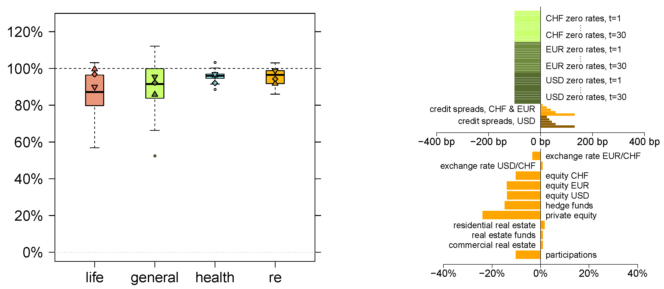
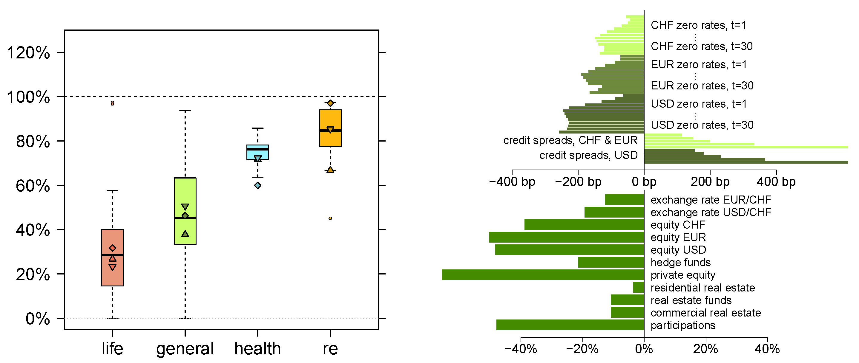
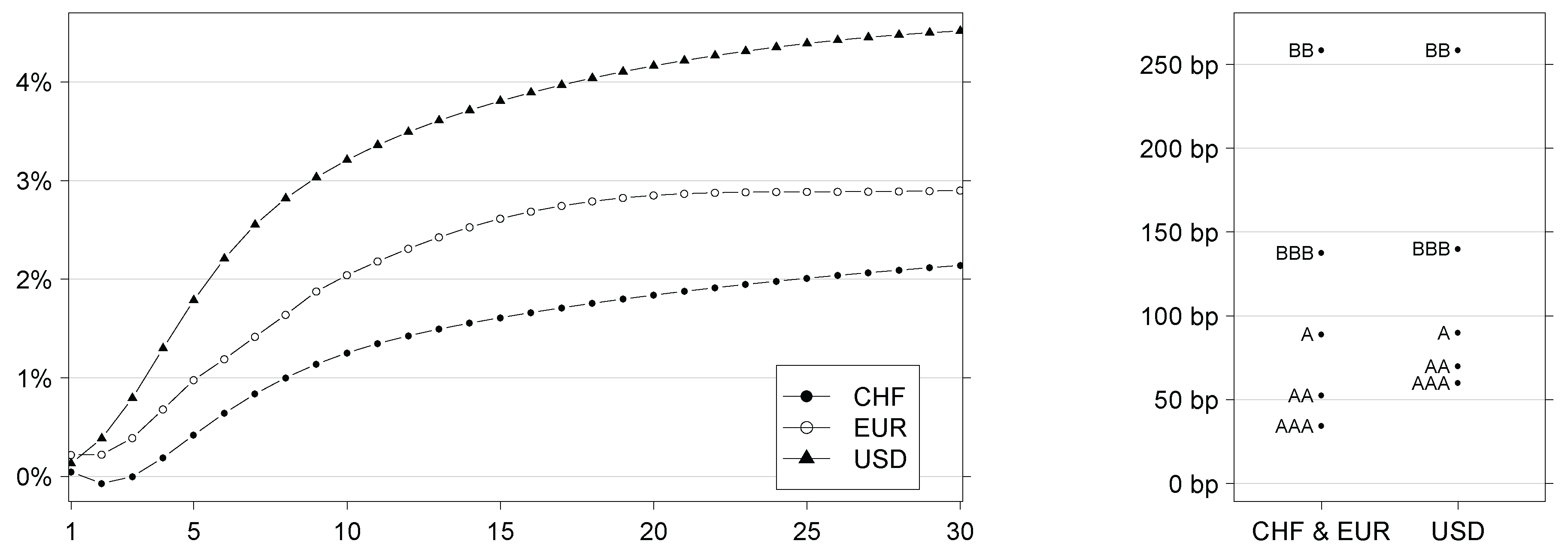
In the figures below we illustrate for each of these scenarios the changes in the market risk factors, see for example Figure 5 (rhs). The predefined changes in market risk factors are colored green, while the conditionally expected changes in the remaining risk factors are colored orange. Absolute changes are shown in basis points (bp) and relative changes in percentages. For a given currency, changes in zero-coupon rates are sorted by maturity $t\in \mathcal{T}$, with maturity $t=1$ year on top. Similarly, for a given currency, changes in credit spreads are sorted by rating $r\in \mathcal{R}\backslash \left\{\mathrm{RF}\right\}$, with rating AAA on top. For better illustration in both cases, zero-coupon rates and credit spreads, we indicate different currencies with different saturations.

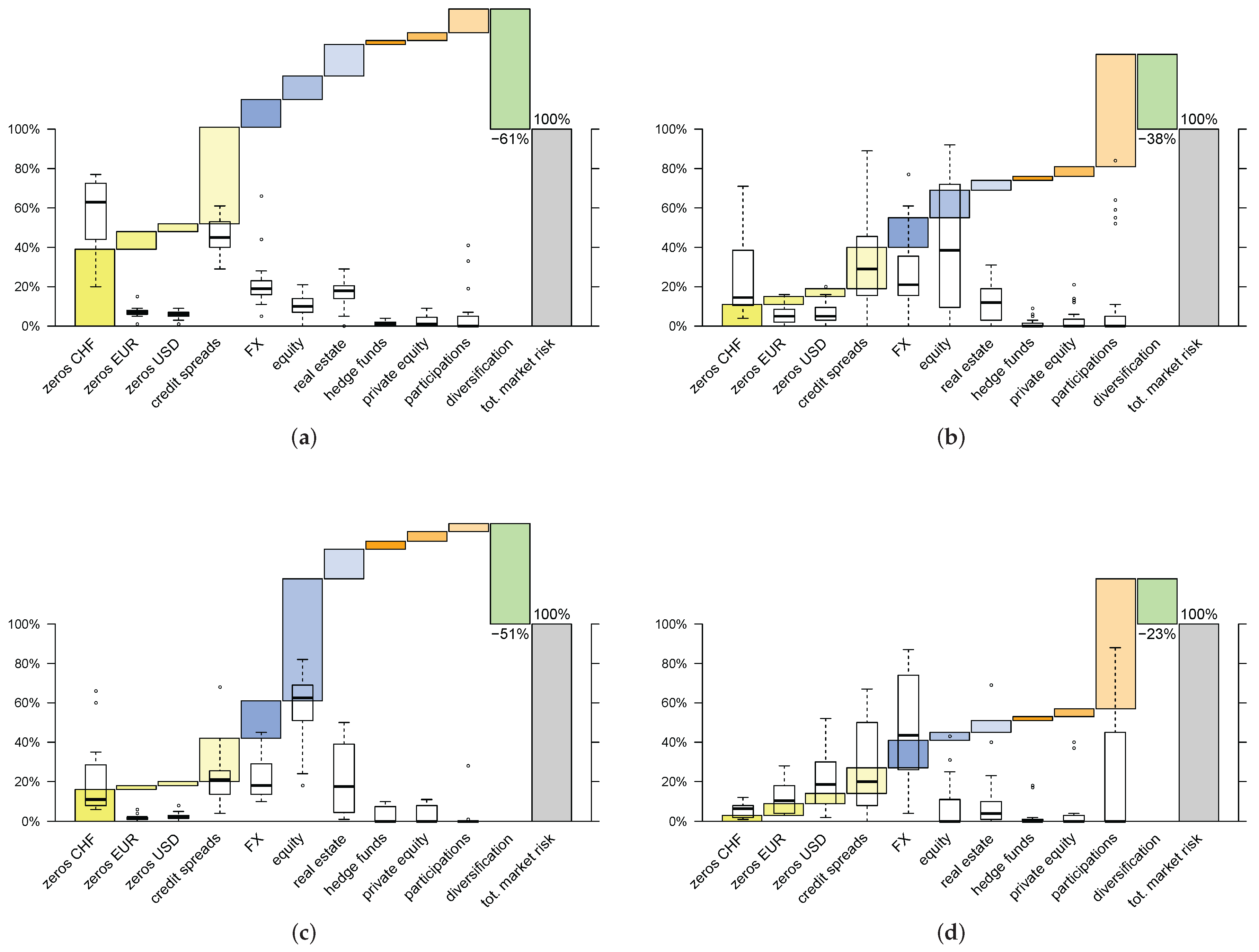
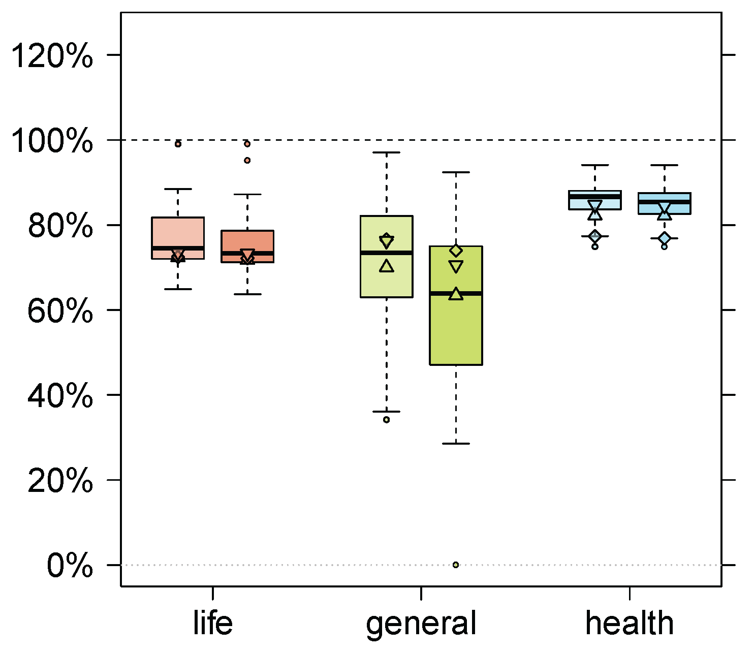
Further, for each stress scenario we present in the same figures box plots summarizing the impact on the CHF insurance market, see for instance Figure 5 (lhs). Each box plot illustrates the impact ratios ${\varrho }_i$ of the companies in a given branch of insurance. The plots colored red correspond to life insurers; we choose green for general insurers, blue for health insurers and we choose orange for reinsurers. Moreover, in each box plot we indicate the impact ratios of the three largest insurers (in terms of balance sheet total) respectively by ▴, ⧫, ▾ in decreasing order, with ▴ indicating the largest insurer.

Decline in risk-free rates. We consider a decrease in each zero-coupon rate by 100 basis points, see green color in Figure 5 (rhs). The market dependencies imply, in particular, an expected increase in credit spreads and an expected decrease in the total values of equity, hedge funds and private equity, see orange color in Figure 5 (rhs). Figure 5 (lhs) illustrates the resulting impact on the CHF insurance market.

The median impact ratio ${\varrho }_i$ for life insurers is $87\%$. The two insurers having almost solely insurance provisions for unit-linked life insurance benefit from this scenario. This is due to the low impact on their respective liability side.

The median impact ratio ${\varrho }_i$ for general insurers is $92\%$. The loss faced by the largest insurer mainly originates from its participation in the life insurer of the CHF insurance network that has an impact ratio of $88\%$. The general insurers with an impact ratio over $100\%$ mainly have insurance provisions for other non-life insurance such as legal protection insurance.

The impact on health insurers and reinsurers is comparably low, with median impact ratios ${\varrho }_i$ of $96\%$ and $97\%$, respectively.

Conclusion. We observe that most of the insurance companies are able to absorb this stress scenario in an adequate way. Therefore, the scenario does not have a severe macroprudential effect on the CHF insurance market.

If, instead, we increase each zero-coupon rate by 100 basis points, we virtually get mirrored plots compared to Figure 5. Note that a considerable rise in interest rates may additionally cascade an increase in lapse rates. This is analyzed separately in Section 5.2.

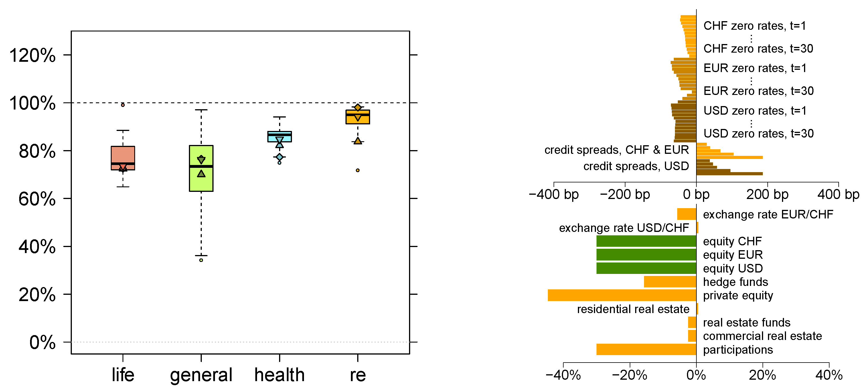
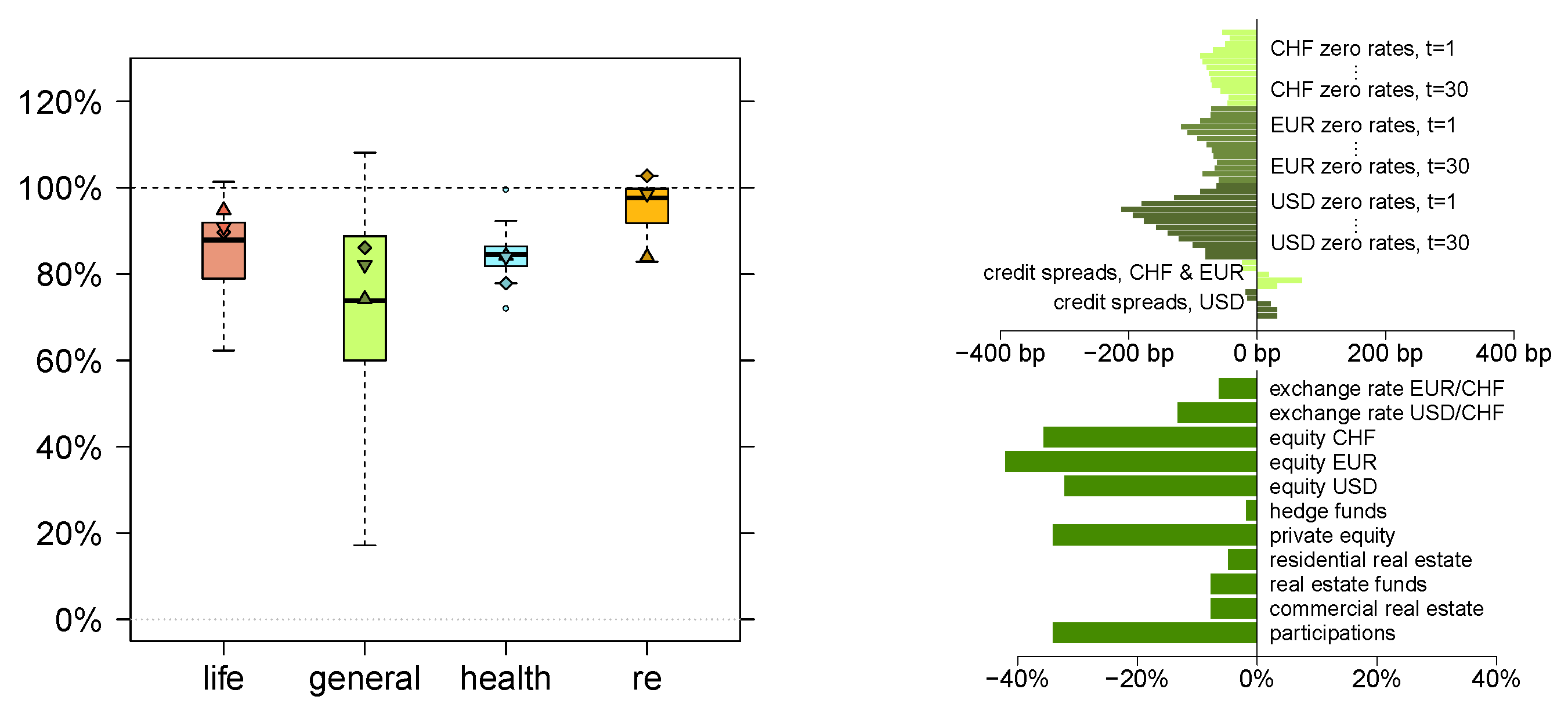
Fall of the equity market. We analyze the impact on the CHF insurance market when the total value in equity drops by $30\%$ for all currencies, see green color in Figure 6 (rhs). The market dependencies imply an expected drop of $45\%$ in total value of private equity, an expected drop of $16\%$ in total value of hedge funds and remarkable changes in risk-free rates and credit spreads, see orange color in Figure 6 (rhs). The impact on the CHF insurance market is illustrated in Figure 6 (lhs).

The median drop in risk bearing capital is $25\%$ for life insurers. This drop is mainly caused by the changes in the risk-free rates and credit spreads. Again, the two life insurers feeling nearly no impact mainly have insurance provisions for unit-linked life insurance.

The median drop in risk bearing capital is $27\%$ for general insurers. This drop mainly stems from losses in equity, collective and alternative investments and, if any, participations in life insurers of the CHF insurance network.

The picture is similar for health insurers, though the corresponding median drop of $13\%$ in own equity is less pronounced. However, the five lowest impact ratios ${\varrho }_i$ belong to the five largest insurers. The impact is low for most reinsurers, with a median impact ratio of $95\%$. The largest reinsurer suffers a loss amounting to $16\%$ of its initial risk bearing capital mainly due to its participations in companies (none of these is part of the CHF insurance network). The outlier with an impact ratio of $72\%$ suffers losses primarily because of its holdings in equity and alternative investments.

Conclusion. This stress scenario has a significant impact on the life insurers of the CHF insurance market. The weighted average of impact ratios is $74\%$ for these insurers. Assuming a weighted average of solvency ratios of $140\%$, this scenario is a severe danger to the life insurance market. Special measures, like a temporary relaxation of solvency requirements, possibly need to be applied in order to ensure the continuous functionality of that market.

The stress scenario has a comparable impact on general insurers and a less severe impact on health insurers and reinsurers. Supported by the high average means of solvency ratios for these branches of insurance, we conclude that the scenario does not pose a great danger to these insurance sectors.

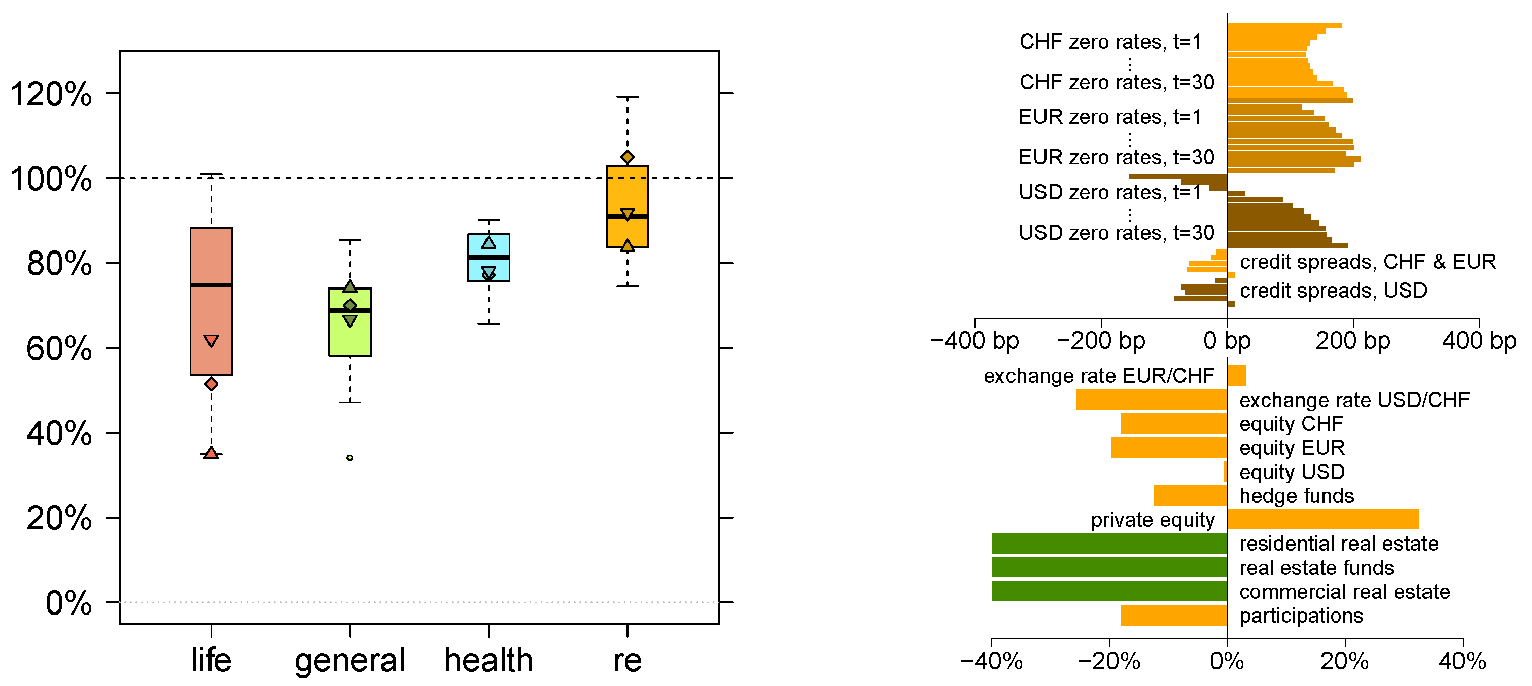
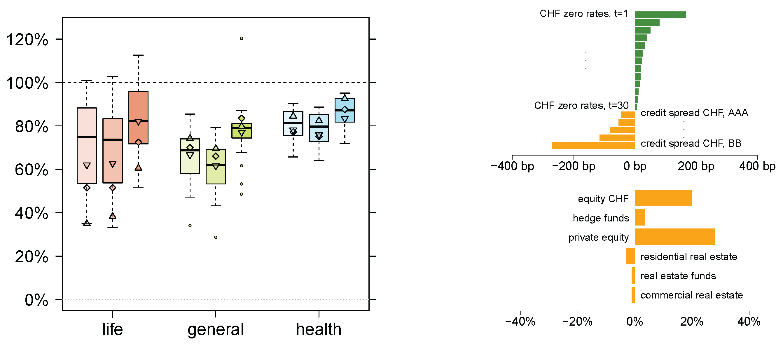
Real estate market crash. Next, we analyze the consequences of a real estate market crash for the CHF insurance market. For this, we set the changes in all real estate related market risk factors to $-40\%$. This decrease can be compared to the real estate crisis in Switzerland in the 1990’s, in which real estate price indexes declined by more than $35\%$, see [36]. The conditionally expected changes in the remaining risk factors and the resulting impact ratios ${\varrho }_i$ are illustrated in Figure 7.

The median impact ratio is $75\%$ for life insurers. In particular the large companies suffer high losses. These losses are mainly caused by real estate related investments. The losses on the asset side and the gains on the liability side due to the changes in interest rates practically compensate each other.

The median impact ratio is $69\%$ for general insurers. These insurers mainly face losses due to their participations (in life insurers of the network) and due to the drawdown of the equity market. For instance, the loss in participations of the largest general insurer contributes 20 percentage points to the drop of $26\%$ in its own equity.

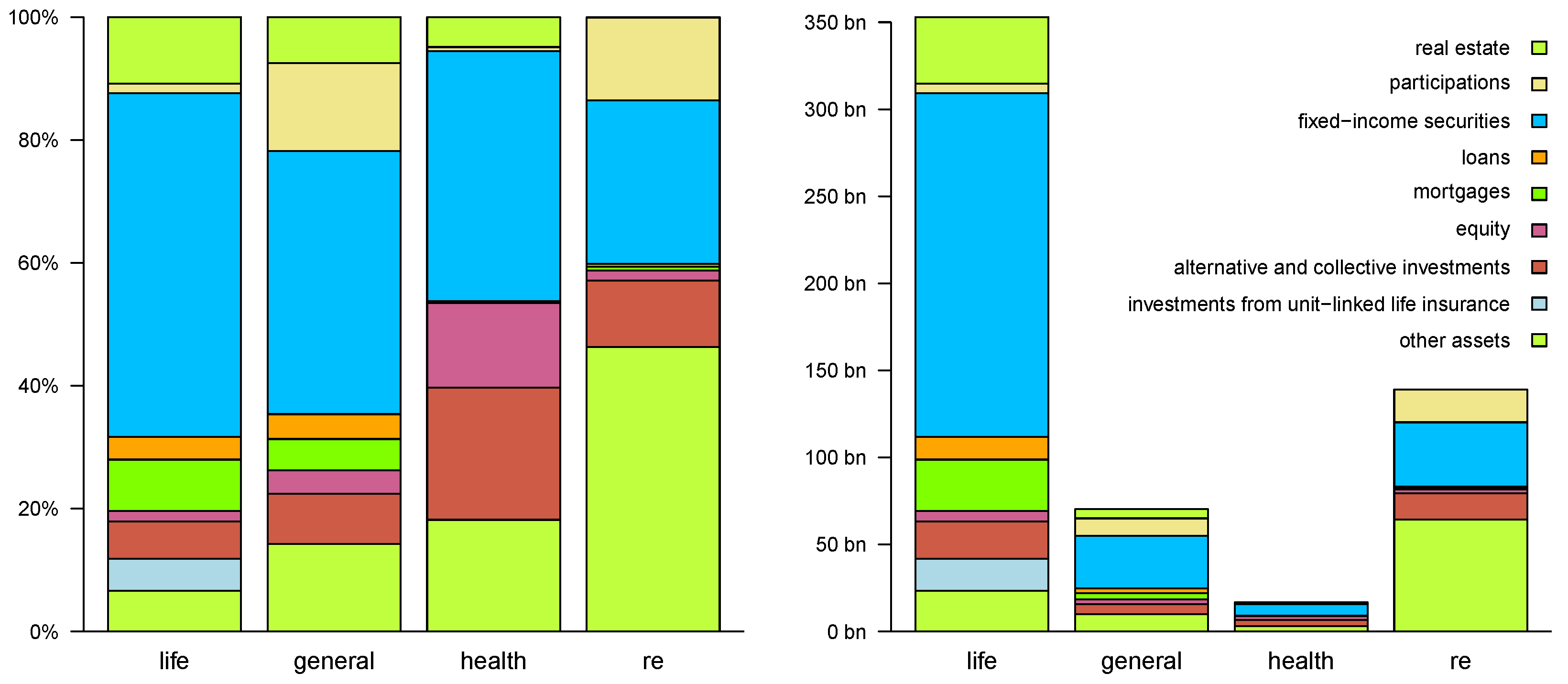
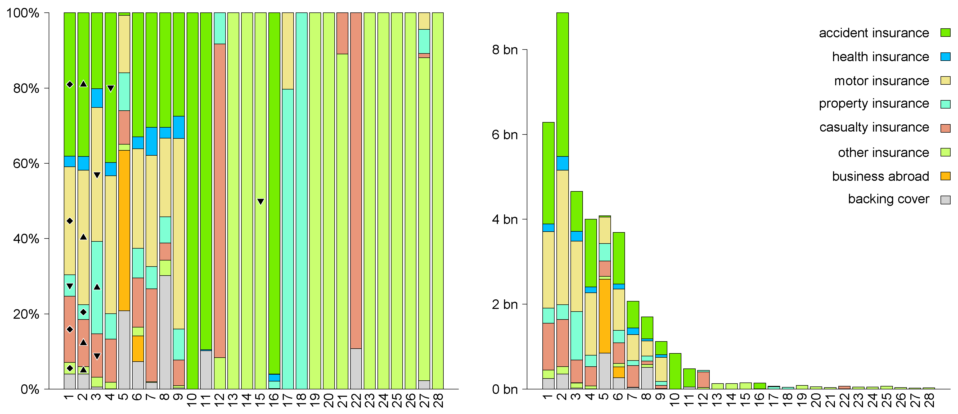
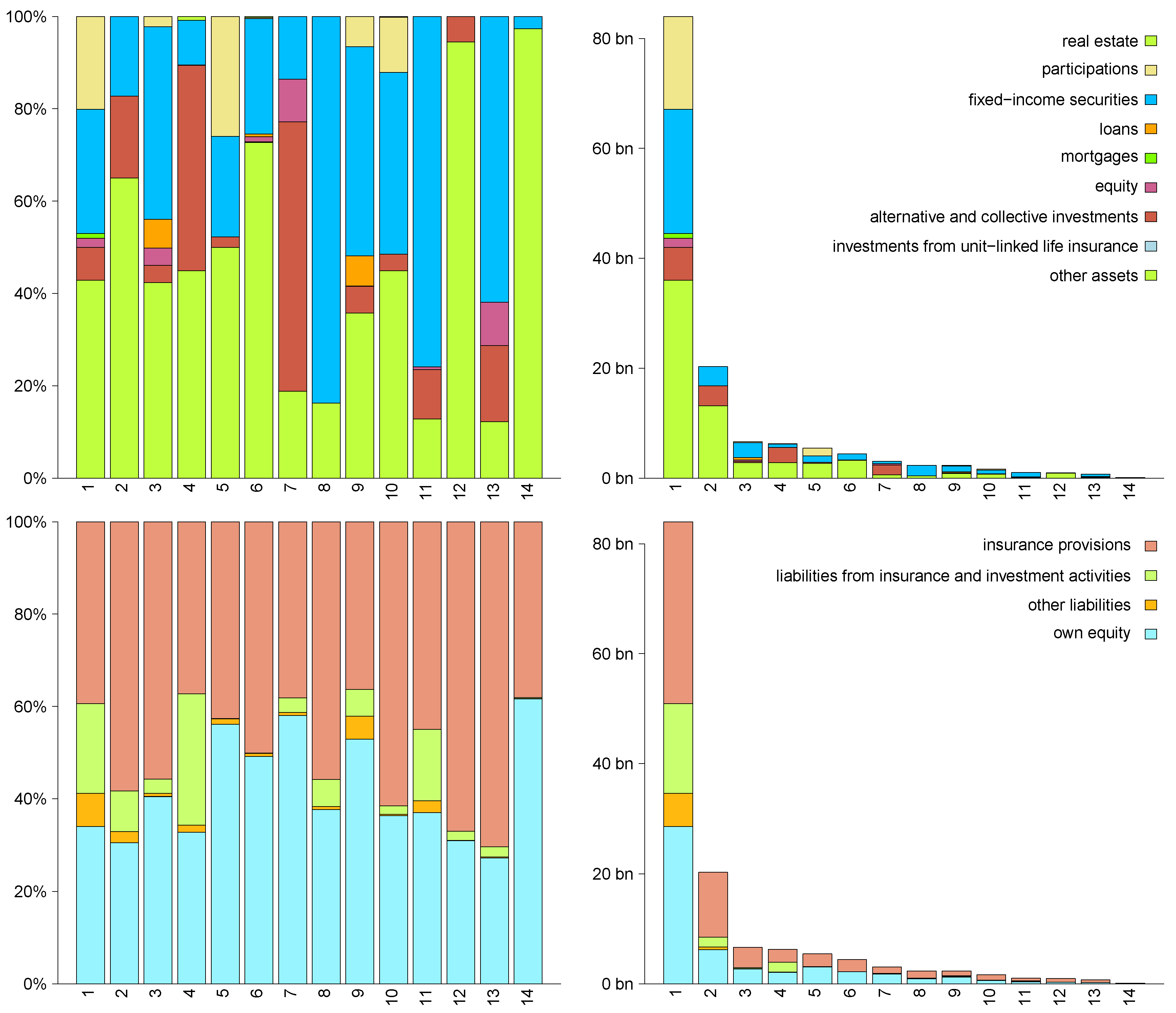
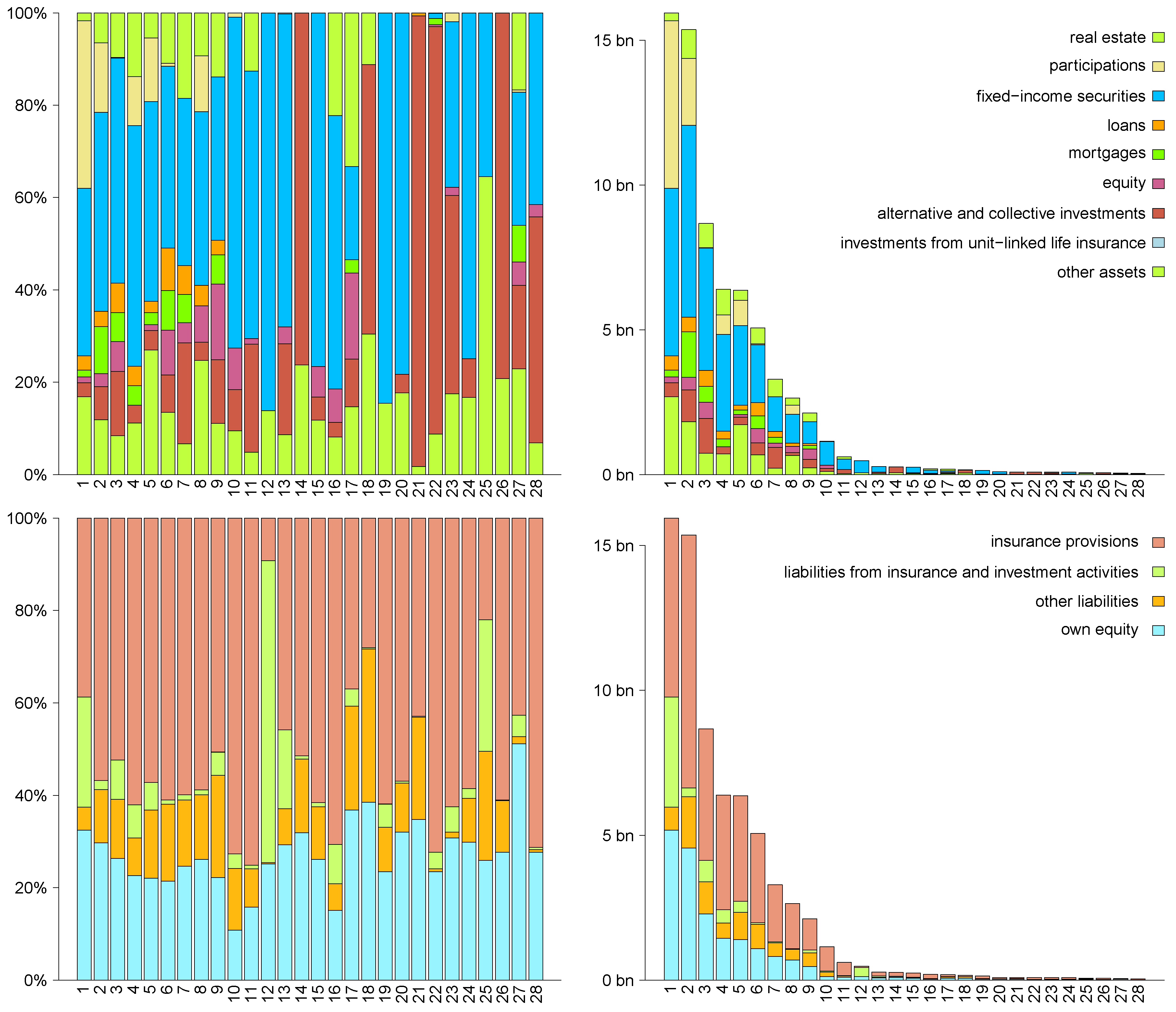
The median impact ratio is $81\%$ for health insurers. The losses primarily originate from real estate related investments and holdings in the equity market. The median impact ratio for reinsurers is $91\%$. Observe that these insurers do not have big investments in real estate, see their balance sheets in Figure A5. Some reinsurers benefit from the scenario due to the increase in risk-free rates.

Conclusion. The real estate market crash defined above has a severe impact on the life insurance sector of the CHF insurance market. Especially the large companies are highly affected by the scenario, the life insurers’ weighted average of impact ratios is $54\%$. Assuming a weighted average of solvency ratios of $140\%$, we conclude that the life insurance market as a whole may not bear a real estate market crash in its current state. The analysis of this stress scenario illustrates that the real estate exposure of (large) life insurers poses a severe danger to the continuous functionality of the life insurance industry.

From a macroprudential point of view a real estate market crash has a severe impact on the general insurance market as well, with a weighted average of impact ratios given by $69\%$. However, the weighted average of solvency ratios for general insurers is sufficiently high in order to appropriately absorb the losses resulting from the scenario.

The impact on health insurers and reinsurers is less pronounced. Additionally, their respective weighted averages of solvency ratios are sufficiently high in order to bear the consequences of a real estate market crash.

Financial crisis as of 2007/2008. We consider a scenario where the market risk factors are stressed according to the financial crisis of 2007/2008. The changes in the risk factors corresponding to this crisis are provided by FINMA [37] and illustrated in Figure 8 (rhs). Credit spreads increase, all other risk factors are negatively shocked. The resulting impact ratios are summarized in Figure 8 (lhs).

The median impact ratio is $28\%$ for life insurers, while three companies face losses larger than their respective risk capacity. For each of these three companies, more than $50\%$ of insurance provisions correspond to reserves in endowment insurance which, in all three cases, increase by roughly $20\%$ due to the decline in risk-free rates. The increase in credit spreads dampen the corresponding gains on the asset side, which finally results in negative own equity for all three insurers. Similar effects hold for the other life insurers, but to a less extent. The two life insurers feeling nearly no impact mainly have insurance provisions for unit-linked life insurance.

The median impact ratio is $45\%$ for general insurers. Three insurers face losses larger than their respective risk bearing capital. For one of these three insurers this is due to the devaluation of holdings in collective investments, which represent $88\%$ of the insurer’s asset side. The other two insurers, as well as a further insurer having an impact ratio of $3\%$, mainly have insurance provisions for (annuities in) accident insurance.

The impact on health insurers is comparably low. However, especially the large companies are highly affected. Generally, health insurers face losses mainly because of their investments in the equity market. The impact on reinsurers is comparably low as well. The loss of the largest reinsurer results from its participations. The outlier having an impact ratio of $45\%$ particularly suffers losses related to its investments in the equity market and holdings in alternative investments.

Conclusion. A financial crisis as of 2007/2008 has a severe impact on most life insurers of the CHF insurance market; the weighted average of impact ratios is $29\%$ for life insurers. Assuming a weighted average of solvency ratios of $140\%$, such a crisis would highly disrupt the continuous functionality of the life insurance industry. We conclude that the life insurance industry in its current state would not survive a financial crisis of size 2007/2008. Of course, we may argue that this scenario is unlikely to happen twice in 10 years. In particular, the current low interest environment does not support another massive decline in the interest rates.

The general insurance market is hit to a less extent. The scenario results in a weighted average of impact ratios of $42\%$. However, assuming a weighted average of solvency ratios of $190\%$, we conclude that a financial crisis of size 2007/2008 is a severe danger to the continuous functionality of the general insurance market.

The impact on health insurers is less pronounced. Although the large insurers are hit particularly by the scenario, the weighted average of solvency ratios for health insurers is sufficiently high in order to appropriately absorb the consequences of a financial crisis as of 2007/2008. This conclusion also holds true for the reinsurance market.

Stock market crash as of 2000/2001. We consider a scenario where the market risk factors are stressed according to the stock market crash of 2000/2001. The changes in the risk factors corresponding to this crash are provided by FINMA [37] and illustrated in Figure 9 (rhs). Note that these changes are similar to the ones corresponding to the financial crisis 2007/2008, see Figure 8 (rhs), but less extreme. Therefore, the losses on the asset side are smaller compared to the previous scenario. The impact ratios in turn look more comforting, see Figure 9 (lhs).

Note that this historical scenario is also similar to the fall of the equity market scenario in Figure 6 (rhs). This supports the choice of the covariance matrix (provided by FINMA) to evaluate Lemma 1, as well as the design of our scenarios.

Conclusion. We observe that the scenario impacts the CHF insurance market similarly to the fall of the equity market scenario, see Figure 6. However, compared to the latter scenario, the life insurance market is hit considerably less extreme (which is due to the rather small changes in credit spreads). We therefore conclude that the CHF insurance market is able to absorb a stock market crash as of 2000/2001 in an adequate way.

5.2. Real Estate Market Crash Together with Cascade Effects

We revisit the real estate market crash scenario from Figure 7. Given both the stressed market situation and the increase in risk-free rates, we additionally consider a cascading increase in lapse rate of 20 percentage points as well as a cascading decline in new business of $50\%$ in life insurance and of $20\%$ in non-life insurance. This first cascade effect implies a further cascade effect. This second cascade effect originates from the sale of assets by life insurers in order to raise the surrender values given by (2). We assume that asset prices are stressed so that they can only be sold at a price which is $\ell =90\%$ of the corresponding value in the balance sheet. Moreover, we assume that each insurer raises the surrender values by selling fixed-income securities with currency CHF. The proportion of assets sold having maturity $t\in \mathcal{T}$ and credit rating $r\in \mathcal{R}$ is according to market liquidity. More precisely, the relative amount of sold fixed-income securities with currency CHF, maturity $t\in \mathcal{T}$ and credit rating $r\in \mathcal{R}$ is given by $A_{\mathrm{bonds}}^{\mathrm{CHF},t,r}/A_{\mathrm{bonds}}^{\mathrm{CHF}}$ (with a small modification if a company has not sufficiently many holdings in these assets). Here, $A_{\mathrm{bonds}}^{\mathrm{CHF}}$ denotes the total market capitalization of fixed-income securities with currency CHF.

Figure 10 (lhs) illustrates the resulting impact ratios for primary insurers. Figure 10 (rhs) shows the changes in the market risk factors in Table 3 implied by the sale of assets (second cascade effect). The changes caused by the price impact are colored green and the changes caused by market dependencies are colored orange.

The cascading surrenders and the cascading decline in new business (first cascade effect) do not substantially change the median impact ratio of $75\%$ (given by the real estate market scenario) for life insurers. The aggregated surrender value in endowment insurance amounts to $78\%$ (median value) of the corresponding insurance provisions. Despite the increase in risk-free rates of the base scenario, this is a peculiarity of the present low interest rate environment. To raise the surrender values, $7.1$ billion CHF are liquidated by selling fixed-income securities with currency CHF. This corresponds to roughly $1.5\%$ of the total market capitalization. The market impact caused by the sale of assets (second cascade effect) implies that some assets gain in value and in turn affect the impact ratios of most life insurers positively. The median impact ratio finally is $82\%$, i.e., we observe an easing of the scenario.

For general insurers, considering the cascading decline in new business and the cascading increase in lapse rates in addition (first cascade effect), the median impact ratio drops to $62\%$. However, due to the sale of assets by life insurers and the resulting changes in market risk factors (second cascade effect), the impact ratios of most general insurers increase again.

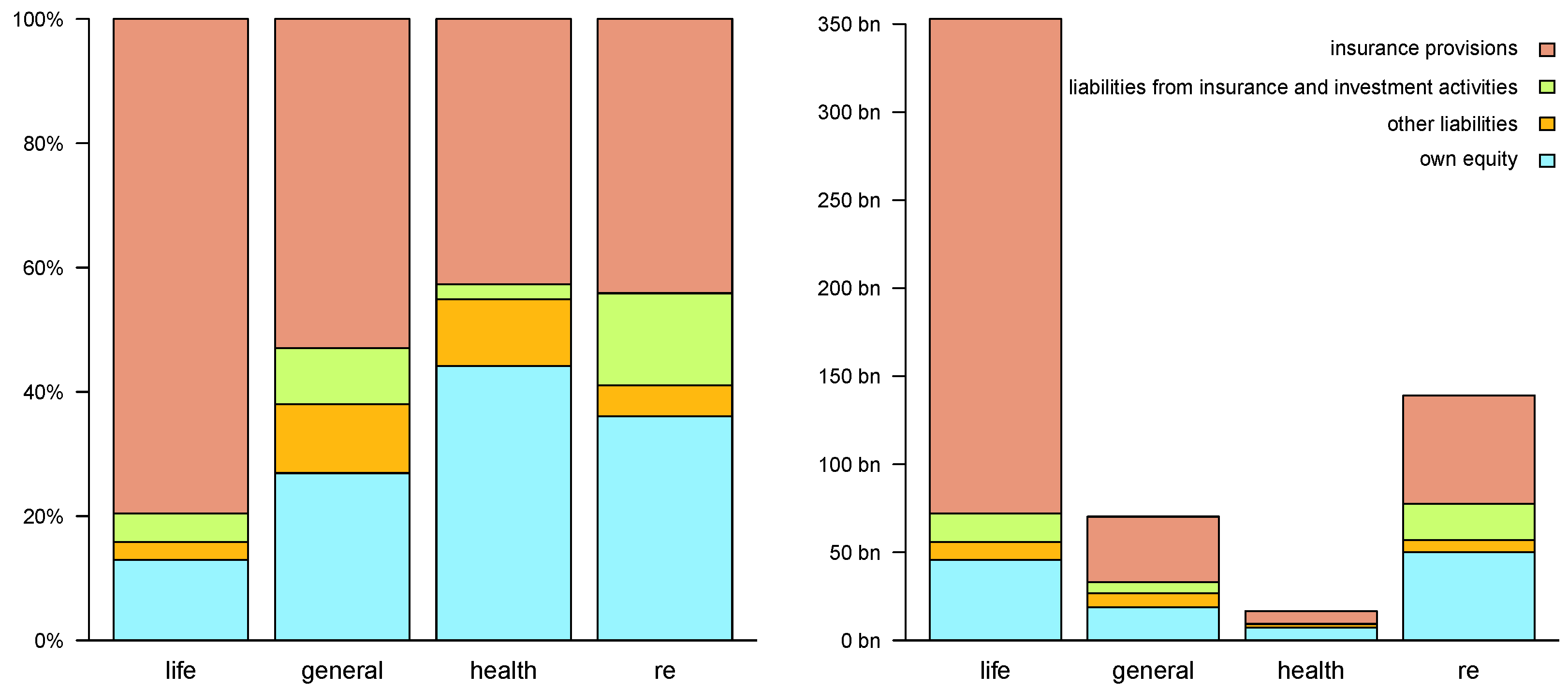
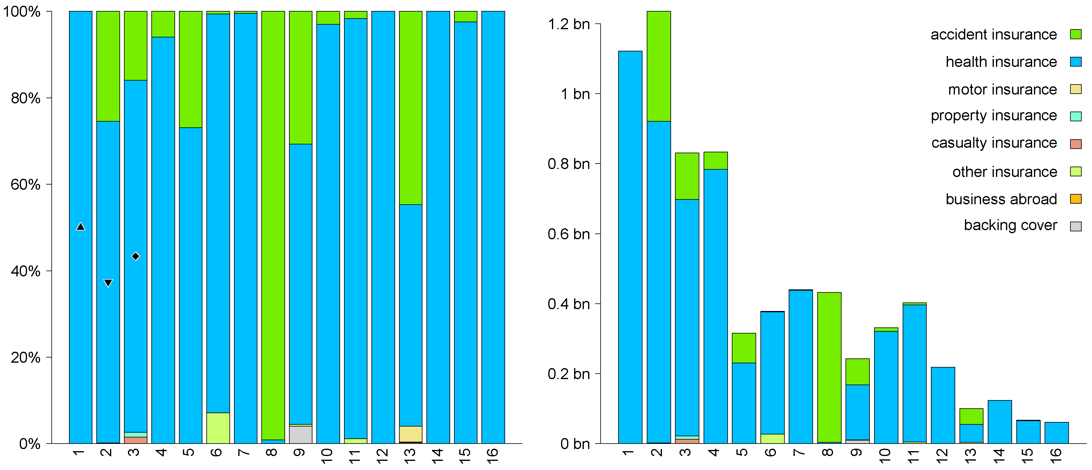
Similarly for health insurers, however, the cascading impact is less pronounced due to their higher risk margins, see their balance sheets in Figure A4. The median impact ratio for these insurers is $87\%$.

Conclusion. The two cascade effects positively influence the solvency results of most life insurers of the CHF insurance market. Especially the market impact (second cascade effect) improves the impact ratios. The resulting weighted average of impact ratios is $73\%$ for life insurers. Recall from Section 5.1 that the real estate market crash without cascade effects results in a weighted average of $54\%$. The cascade effects therefore significantly dampen the impact of a real estate market crash in our model. This is a peculiarity of the present low interest rate environment and should not be generalized to other market environments.

The market impact triggered by the sale of assets by life insurers (second cascade effect) positively affect the solvency results of most general and health insurers. In particular, despite the losses from the decline in new business (first cascade effect), the two cascade effects dampen the impact of a real estate market crash on the general and health insurance sector of the CHF insurance market.

5.3. Failure of Reinsurers in a Stressed Market Situation

In this section we analyze the consequences for the CHF insurance market of a cascading failure of reinsurers, given a disruption of the financial market. We consider the fall of the equity market scenario given in Figure 6 (rhs) as a base scenario. Because of the stressed market situation, we assume that not every reinsurer is able to meet its obligations. As cascade effect we think of the global reinsurer introduced in Section 4 can only cover $50\%$ of the total reinsured liabilities ${\mathcal{V}}_i\left(r\right)$ of each company i. We model the loss faced by primary insurer i by

$$50\%·{\mathcal{V}}_i\left(r\right)+50\%·{\mathcal{V}}_i\left(p_{\mathrm{re}}\right),$$

where $50\%·{\mathcal{V}}_i\left(p_{re}\right)$ models the costs for buying new reinsurance coverages, which we assume to be available on the global reinsurance market. We also assume that there are no other open claims against reinsurers on the asset side of each insurer’s balance sheet. Figure 11 recalls the impact ratios for the fall of the equity market, see also Figure 6 (lhs), and additionally presents the impact ratios after the cascade effect.

The reinsured liabilities only amount to $0.3\%$ of the gross liabilities on average for life insurers. Therefore, the additional impact caused by the cascading failure of reinsurers is rater low. The median impact ratio drops by roughly one percentage point to $73\%$ for life insurers.

When considering the cascading failure of reinsurers additionally, the median of impact ratios drops from $73\%$ to $64\%$ for general insurers. These insurers of the CHF insurance market reinsure $10\%$ of gross liabilities on average. However, there are two insurers with reinsured liabilities that amount to $90\%$ and $80\%$ of gross liabilities, respectively. Their impact ratios of $95\%$ and $97\%$, respectively, given by the base scenario drop to $0\%$ each because of the cascade effect.

Similarly to life insurers, the additional impact from the cascade effect is low for health insurers. This is due to the fact that reinsured liabilities only amount to $0.7\%$ of gross liabilities on average for the health insurers of the CHF insurance market.

Conclusion. This stress scenario illustrates that the failure of reinsurers does not impact the life and health insurance market to a great extent. In particular for the life insurance sector of the CHF insurance market, the cascading failure of reinsurers does not remarkably amplify the threatening impact of a fall of the equity market.

Many general insurers face significant losses caused by the cascading failure of reinsurers. The weighted average of impact ratios is $63\%$ for general insurers. However, assuming a weighted average of solvency ratios of $190\%$, we conclude that a fall of the equity market combined with the cascading failure of reinsurers may still be absorbed by the general insurance industry. This stress scenario in particular illustrates to what extent a cascading failure of reinsurers amplifies the initial impact on the general insurance sector caused by a disruption of the financial market.

5.4. Longevity and Underreserving

In this section we analyze the impact on direct insurers when mortality rates are decreased and when insurance provisions for non-life insurance additionally have to be increased. A joint reserve strengthening may be motivated by changes in legislation. Furthermore, we assume that this reserve strengthening cascades a decline in new business. This might be motivated by mistrust in insurance companies or by an increase in price levels of premiums as a consequence of the reserve strengthening.

In the following we assume that the mortality rates $q_{x,t}$ are changed according to (1) with $\mathrm{\Delta }{Z}^{\lambda }=100\%$ and with ${\lambda }_{x,t}=t\log \left(2\right)/\max \{40,x\}$ for $x\in \mathbb{N}$ and $t\ge 0$, see also [38]. Therefore, the insurance provisions of a company are revalued by using the new mortality rates given by

$${\tilde{q}}_{x,t}=q_{x,0}{e}^{-2{\lambda }_{x,t}}=q_{x,t}{e}^{-{\lambda }_{x,t}},$$

for $x\ge 65$ and $t\ge 1$, and ${\tilde{q}}_{x,t}=q_{x,t}$, else. This change in mortality rates has comparable size to the longevity scenario considered for solvency requirements in the SST, see [39]. Additionally, we increase the insurance provisions in non-life insurance by $10\%$ for each company. As a cascade effect we consider a decline in new business of $25\%$ in all lines of business.

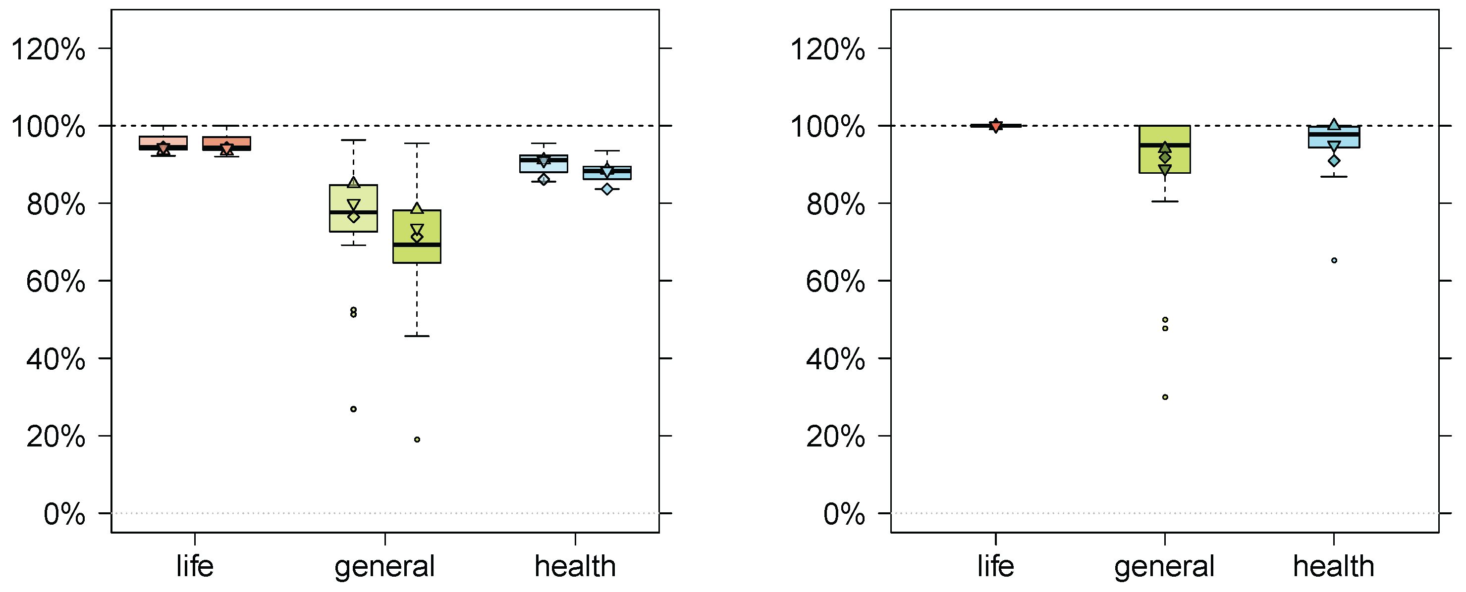
Figure 12 (lhs) illustrates the resulting impact ratios for primary insurers. The left plots only considers the decline in mortality rates and the reserve strengthening. The right plots additionally consider the cascading decline in new business.

For life insurers, the median of impact ratios is $94\%$ for the scenario considering only the decline in mortality rates. The impact of the cascading decline in new business is small. This is because the earned premium in new business is typically low compared to the total earned premium.

For general insurers, the median impact ratio is $78\%$ when considering the reserve strengthening and the decrease in mortality rates only. The lowest three impact ratios in general insurance belong to firms which considerably have insurance provisions for annuities in accident insurance. Hence, they face losses also because of the decrease in mortality rates. Considering the decline in new business as cascade effect, the median impact ratio drops to $69\%$.

Similarly for health insurers, however, the impact is less pronounced due to their higher risk margins, see their balance sheets in Figure A4. The median impact ratio for these insurers is $88\%$.

Conclusion. The life insurers of the CHF insurance market are able to absorb a reserve strengthening caused by a decrease in mortality rates in an appropriate way. The cascading decline in new business has a low additional impact on these insurers.

The reserve strengthening combined with the cascading decline in new business has a significant impact on most general insurers. However, we conclude that from a macroprudential point of view the general insurance market is able to absorb the reserve strengthening and its cascade effect in an adequate way. This is supported by the high solvency ratios of the general insurers.

The impacts of the reserve strengthening and the cascading decline in new business are less extreme for health insurers because of their high capital buffers.

5.5. Terrorist Attack

We consider an event that is motivated by a possible terrorist attack in Switzerland, for example, at Zurich central railway station with roughly 450,000 travelers a day, see [40]. The attack together with the chaotic and disastrous situation results in many deaths as well as injured and disabled people.

We assume that 500 people die, 500 get fully disabled and 2,500 people additionally get injured. $40\%$ of the deaths leave a spouse behind, to which a yearly widow annuity of 32,000 CHF is paid on average. Female spouses are aged 38, while male spouses are aged 42. Moreover, every spouse has $0.75$ children on average, each of these children is aged 16 and receives a yearly orphan’s pension of 12,000 CHF on average. Each disabled person is aged 40 and receives a yearly disability annuity of 64,000 CHF on average. Moreover, we assume that the nominal value of all types of annuities above is increased by $1\%$ every year. Additionally, each injured person costs the corresponding insurance company 20,000 CHF. The resulting costs are then carried by general and health insurers proportional to their market shares in accident insurance, based on earned premiums. Finally, we consider a property damage of 600 million CHF (net of reinsurance) that is covered by these insurers proportional to their market shares in property and casualty insurance. Note that some of the affected people may have life insurance and there might be claims arising from interruption of business, which is not considered for this scenario. Additionally, we assume that the shock at the financial market evaporates quickly with no sustainable effect. Therefore, the total market capitalizations of assets are not affected by this scenario.

This scenario is comparable in size to a similarly motivated catastrophic event considered by the Swiss Federal Office for population protection, see [41]. The total costs of the scenario above amount to $2.14$ billion CHF. Figure 12 (rhs) illustrates the impact ratios for primary insurers. By assumption there is no impact on life insurers. The median impact ratio restricted to those general insurers facing a loss is $90\%$. The three outliers with impact ratios $50\%$, $48\%$ and $30\%$, respectively, have a combined market share in accident insurance of less than $10\%$.

For health insurers, the median impact ratio is $96\%$ when considering only those insurers facing a loss. The lowest impact ratio of $65\%$ belongs to the health insurer with the highest market share in accident insurance ($7\%$) among all health insurers.

Conclusion. The impact of the event described above does not disrupt the CHF insurance market to a great extent. The analysis illustrates that for the absorption of such an impact, the CHF insurance market has a sufficiently low market concentration and its companies have sufficiently high capital buffers. Recall that this is under the assumption that there is no sustainable disruption of the financial market and the economy.

5.6. Pandemic Event and a Big Earthquake

We forgo modeling in detail the impact on the CHF insurance market caused by a pandemic event. To quantify the implied losses faced by an insurer needs detailed knowledge about its contracts underwritten. However, the total loss restricted to Switzerland resulting from an influenza can be estimated, see for instance [42]. In the analysis of [42], roughly $4.5$ million out of $7.2$ million Swiss habitants (as of year 2000) are affected by an influenza, with roughly 20,000 deaths aged between 15 and 65 and roughly 17,300 deaths aged above 65.

The total costs of illness sum up to approximately $2.3$ billion CHF, from which about 400 million CHF correspond to costs to the health care system. Note that a proportion of these latter costs would be carried by health insurance funds, which are not part of the CHF insurance market (recall that we only consider supplementary health insurance companies). The remaining costs of about $1.9$ billion CHF stem from absence from work.

Additionally, a pandemic event would possibly cascade a disruption of the global financial market leading to further losses. FINMA [39] provides changes in the market risk factors caused by a pandemic event. These changes are comparable to the ones corresponding to a fall of the equity market, see Figure 6 (rhs).

We also refrain from detailed modeling of the impact on the CHF insurance market resulting from a severe earthquake. The Swiss Seismological Service estimates that the financial costs caused by an earthquake of magnitude $6.5$ to 7, occurring in Switzerland roughly once every 1500 years, would be around 50 to 100 billion CHF. However, a large proportion of this loss would not be insured, since most insurers in Switzerland do not offer insurance against earthquakes and there does not exist compulsory earthquake insurance. A severe earthquake may also disrupt the whole economy and industry, and recovery can only be managed by a general political initiative of the whole country. For information about the consequences of a big earthquake in Switzerland we refer to [43,44].

6. Conclusions

In this case study we have considered an insurance market, called CHF insurance market, that has features similar to those of the Swiss private insurance market. The basis of this CHF insurance market is publicly available data from the Swiss market. We have analyzed the vulnerability of this market to different risks and shocks from a macroprudential perspective. This analysis is based on stress scenarios related to financial market risks and insurance risks. Additionally, for these scenarios we have considered potential cascade effects arising from policyholder behavior and from the network structure of the insurance market. We have analyzed in detail how these scenarios and cascade effects impact the balance sheets of the insurance companies.

The analysis has shown that the CHF insurance market is able to appropriately absorb scenarios related to insurance risk, such as longevity risk and the risk of underreserving. Therefore, from a macroprudential point of view, these scenarios do not essentially disrupt the CHF insurance market. An exception would be for an event with much wider economic consequences like a severe earthquake.

In particular for the life insurance sector of the CHF insurance market, we have observed a significant sensitivity to disruptions of the financial market. For two of the financial stress scenarios considered the life insurance market is not able to fully absorb the related losses. The continuous functionality of the life insurance industry is most likely not guaranteed under these two scenarios. One of these scenarios is a real estate market crash, in which especially the big companies are highly affected because of their large real estate exposures. Given this event, a temporary relaxation of solvency requirements or other regulatory measures need to be applied in order to support the solvency results of these insurers and, in turn, to ensure the continuous functionality of the life insurance industry. The second scenario which cannot be absorbed by the life insurance market of our model is a financial crisis of size 2007/2008. However, it is likely that a crisis with similar changes in the interest rates does not occur in the current low interest rate situation.

Also the general insurance sector of the CHF insurance market is vulnerable to financial stress scenarios. However, in comparison to the life insurance industry, this sector has a sufficiently high risk capacity to absorb most of the financial scenarios considered. An exception would be for a financial crisis of size 2007/2008 which poses a great danger to the continuous functionality of the general insurance market of our model.

From a macroprudential perspective, the health insurance and reinsurance sector of the CHF insurance market are less exposed to the consequences of financial market stress scenarios. This is supported by the high risk capacities of these insurers.

We have demonstrated that cascading effects may dampen the impact of financial market stress scenarios on the CHF insurance market. Given a disruption of the financial market, we have observed that the sale of assets by life insurers triggered by unexpectedly high lapse rates may cascade a market impact that dampens the initial impact for most companies in all insurance branches. Furthermore, we have observed that the consequences of a failure of reinsurers may be absorbed by the CHF insurance market. However, given a stressed market situation, a cascading failure of reinsurers may amplify the financial distress in such a way that the continuous functionality of the general insurance market is not necessarily guaranteed.

References

1. FINMA. Technisches Dokument zum Swiss Solvency Test. Version 02. Oktober 2006. Bern, Switzerland: Eidgenössische Finanzmarktaufsicht FINMA, 2006. [Google Scholar]
2. A. French, M. Vital, and D. Minot. “Insurance and Financial Stability.” In Quarterly Bulletin 2015 Q3. London, UK: Bank of England, 2015. [Google Scholar]
3. FINMA. “Elektronische Tabellen über den Versicherungsmarkt, 2015.” Eidgenössische Finanzmarktaufsicht FINMA. Available online: http://www.versichererreport.finma.ch (accessed on 12 December 2016).
4. Bank of England. Procyclicality and Structural Trends in Investment Allocation by Insurance Companies and Pension Funds: A Discussion Paper by the Bank of England and the Procyclicality Working Group. London, UK: Bank of England, 2014. [Google Scholar]
5. Swisscanto. Schweizer Pensionskassenstudie 2016. Zurich, Switzerland: Swisscanto Vorsorge AG, 2016. [Google Scholar]
6. M. Eling, and D. Pankoke. Systemic Risk in the Insurance Sector: Review and Directions for Future Research. Working Papers on Finance; St. Gallen, Switzerland: Institute of Insurance Economics, University of St. Gallen, 2014, Volume 21. [Google Scholar]
7. IAIS. Insurance and Financial Stability, 2011. Basel, Switzerland: International Association of Insurance Supervision, 2011. [Google Scholar]
8. R.W. Klein. “Insurance Market Regulation: Catastrophe Risk, Competition, and Systemic Risk.” In Handbook of Insurance. New York, NY, USA: Springer, 2013, pp. 909–939. [Google Scholar]
9. J.D. Cummins, and M.A. Weiss. “Systemic risk and the U.S. insurance sector.” J. Risk Insur. 81 (2014): 489–528. [Google Scholar] [CrossRef]
10. G.N. Weiss, and J. Mühlnickel. “Why do some insurers become systemically relevant? ” J. Financ. Stab. 13 (2014): 95–117. [Google Scholar] [CrossRef]
11. D. Kessler. “Why (re)insurance is not systemic.” J. Risk Insur. 81 (2014): 477–488. [Google Scholar] [CrossRef]
12. T. Adrian, and M.K. Brunnermeier. CoVaR. Working Paper 17454; Cambridge, MA, USA: National Bureau of Economic Research, 2011. [Google Scholar]
13. M. Billio, M. Getmansky, A.W. Lo, and L. Pelizzon. “Econometric measures of connectedness and systemic risk in the finance and insurance sectors.” J. Financ.Econ. 104 (2012): 535–559. [Google Scholar] [CrossRef]
14. C. Brownlees, and R.F. Engle. “SRISK: A conditional capital shortfall measure of systemic risk.” Rev. Financ. Stud., 2016. [Google Scholar] [CrossRef]
15. E. Berdin, and M. Sottocornola. “Insurance Activities and Systemic Risk, 2015.” Available online: https://ssrn.com/abstract=2701821 (accessed on 12 December 2016).
16. I. Alves, J. Brinkhoff, S. Georgiev, J.C. Héam, I. Moldovan, and M. Scotto di Carlo. Network Analysis of the EU Insurance Sector. Frankfurt am Main, Germany: ESRB Occasional Paper, 2015, Number 7. [Google Scholar]
17. K. Nyholm. “Insurance and banking interconnectedness in Europe: The opinion of equity markets.” Econ. Res. Int. 2012 (2012): 525089. [Google Scholar] [CrossRef]
18. T.R. Hurd. Contagion! The Spread of Systemic Risk in Financial Networks. Cham, Switzerland: SpringerBriefs in Quantitative Finance, Springer International Publishing, 2016. [Google Scholar]
19. J. Monkiewicz, and M. Małecki. Macroprudential Supervision in Insurance: Theoretical and Practical Aspects. London, UK: Palgrave Macmillan, 2014. [Google Scholar]
20. A. Jobst, N. Sugimoto, and T. Broszeit. Macroprudential Solvency Stress Testing of the Insurance Sector. IMF Working Papers; Washington, DC, USA: International Monetary Fund, 2014, Volume 24. [Google Scholar]
21. C. Christophersen, and J. Zschiesche. Macroprudential Objectives and Instruments for Insurance—An Initial Discussion. EIOPA Financial Stability Report—May 2015; Frankfurt am Main, Germany: European Insurance and Occupational Pensions Authority, 2015, pp. 72–90. [Google Scholar]
22. S.E. Harrington. “The financial crisis, systemic risk, and the future of insurance regulation.” J. Risk Insur. 76 (2009): 785–819. [Google Scholar] [CrossRef]
23. The Geneva Association. Systemic Risk in Insurance—An Analysis of Insurance and Financial Stability, 2010. Zurich, Switzerland: The Geneva Association, 2010. [Google Scholar]
24. The Geneva Association. Key Financial Stability Issues in Insurance—An Account of The Geneva Association’s Ongoing Dialogue on Systemic Risk with Regulators and Policy-Makers, 2010. Zurich, Switzerland: The Geneva Association, 2010. [Google Scholar]
25. H. Chen, J.D. Cummins, K.S. Viswanathan, and M.A. Weiss. “Systemic risk and the interconnectedness between banks and insurers: An econometric analysis.” J. Risk Insur. 81 (2014): 623–652. [Google Scholar] [CrossRef]
26. M.P. Radice. Assessing the Potential for Systemic Risks in the Insurance Sector: Considerations on Insurance in Switzerland. FINMA Working Paper; Bern, Switzerland: Eidgenössische Finanzmarktaufsicht FINMA, 2010. [Google Scholar]
27. IMF. Germany: Financial Sector Assessment Program: Stress Testing the Banking and Insurance Sectors—Technical Notes. IMF Country Report; Washington, DC, USA: International Monetary Fund, 2016, Volume 16. [Google Scholar]
28. EIOPA. EIOPA Insurance Stress Test 2014. EIOPA–BOS; Frankfurt am Main, Germany: European Insurance and Occupational Pensions Authority, 2014, Volume 203. [Google Scholar]
29. ESRB. Report on Systemic Risks in the EU Insurance Sector, 2015. Frankfurt am Main, Germany: European Systemic Risk Board, 2015. [Google Scholar]
30. FINMA. “Standardmodell Schadenversicherung, 2015.” Eidgenössische Finanzmarktaufsicht FINMA. Latest Version. Available online: https://www.finma.ch/de/ueberwachung/versicherungen/spartenuebergreifende-instrumente/schweizer-solvenztest-sst (accessed on 12 December 2016).
31. FINMA. “Wegleitung zum SST-Marktrisiko-Standardmodell, 2014. Ausgabe vom 23. Dezember 2014.” Eidgenössische Finanzmarktaufsicht FINMA. Latest Version. Available online: https://www.finma.ch/de/ueberwachung/versicherungen/spartenuebergreifende-instrumente/schweizer-solvenztest-sst (accessed on 12 December 2016).
32. A.J. McNeil, R. Frey, and P. Embrechts. Quantitative Risk Management: Concepts, Techniques and Tools. Princeton Series in Finance; Princeton, NJ, USA: Princeton University Press, 2015. [Google Scholar]
33. F. Caccioli, M. Shrestha, C. Moore, and J.D. Farmer. “Stability analysis of financial contagion due to overlapping portfolios.” J. Bank. Financ. 46 (2014): 233–245. [Google Scholar] [CrossRef]
34. J. Blanchet, and Y. Shi. “Stochastic Risk Networks: Modeling, Analysis and Efficient Monte Carlo, 2012.” Available online: https://ssrn.com/abstract=2012987 (accessed on 12 December 2016).
35. FINMA. “SST 2014 survey: FINMA report on the Swiss insurance market, 2014.” Bern, Switzerland: Eidgenössische Finanzmarktaufsicht FINMA, 2014. [Google Scholar]
36. SNB. “Real Estate Price Indices – Total for Switzerland, 2016.” Swiss National Bank Data Portal. Available online: https://data.snb.ch/de/topics/uvo#!/cube/plimoincha (accessed on 12 December 2016).
37. FINMA. “Financial Market Scenarios Template for SST, 2015.” Bern, Switzerland: Eidgenössische Finanzmarktaufsicht FINMA, 2014. [Google Scholar]
38. P. Nolfi. “Die Berücksichtigung der Sterblichkeitsverbesserung in der Rentenversicherung nach der Optimalmethode der Spieltheorie.” Mitt. Ver. Schweiz. Versicher. 59 (1959): 29–48. [Google Scholar]
39. FINMA. “Wegleitung Betreffend Szenarien und Stresstests im SST, 2014. Ausgabe vom 31. Oktober 2014.” Eidgenössische Finanzmarktaufsicht FINMA. Latest Version. Available online: https://www.finma.ch/de/ueberwachung/versicherungen/spartenuebergreifende-instrumente/schweizer-solvenztest-sst (accessed on 12 December 2016).
40. SBB. Die SBB in Zahlen und Fakten, 2015. Bern, Switzerland: Schweizerische Bundesbahnen AG, 2015. [Google Scholar]
41. BABS. “Nationale Gefährdungsanalyse—Gefährdungsdossier Konventioneller Anschlag, 2015.” Schweizer Eidgenossenschaft. Bundesamt für Bevölkerungsschutz. Available online: www.babs.admin.ch/de/aufgabenbabs/gefaehrdrisiken/natgefaehrdanalyse/gefaehrddossier.html (accessed on 12 December 2016).
42. J. Piercy, and A. Miles. The Economics of Pandemic Influenza in Switzerland, 2003. Liebefeld, Switzerland: Swiss Federal Office of Public Health, 2003. [Google Scholar]
43. Schweizerische Rückversicherungs-Gesellschaft Zürich. “Versicherungsdeckungen sind heute unzureichend. Was, wenn in der Schweiz die Erde bebt? ” Zurich, Switzerland: Swiss Re Publishing, 2000. [Google Scholar]
44. SVV. Die Flächendeckende Erdbebenversicherung, 2008. Zurich, Switzerland: Schweizerischer Versicherungsverband, 2008. [Google Scholar]
• 1.Only supplementary health insurance companies are considered, because basic health insurance is run like social insurance in Switzerland.
Figure 1. Market shares based on earned premiums of the three largest Swiss insurers in selected lines of business in year 2014, see [3]. The values shown are additive and different colors reflect different insurers/groups.
Risks 04 00047 g001
Figure 2. Asset allocations of 11 large Swiss life insurers by the end of year 2014, see [3]. The values shown are in percentage (lhs) and in billion Swiss franc (rhs), respectively.
Risks 04 00047 g002
Figure 3. Zero-coupon rates r w , t (lhs) and credit spreads s w , r (rhs) considered for the case study.
Risks 04 00047 g003
Figure 4. Market risk analysis of the CHF insurance market based on the Swiss Solvency Test (SST) guidelines. On the level of a single company, this analysis provides the contributions of selected market risk factors to the total market risk. Each box plot considers all companies in a given branch of insurance individually. The superimposed waterfall diagram illustrates weighted averages over all companies in a given branch of insurance. These diagrams also show the weighted average diversification effect for each branch of insurance. (a) life insurance; (b) general insurance; (c) health insurance; (d) reinsurance.
Risks 04 00047 g004
Figure 5. (rhs) illustrates the changes in market risk factors due to a decline in all zero-coupon rates. The changes colored green are predefined, the changes colored orange result from market dependencies. (lhs) illustrates the resulting impact ratios ϱ i of the insurance companies, where ▴, ⧫ and ▾ correspond to the impact ratios of the first, second and third largest company, respectively, in each branch of insurance.
Risks 04 00047 g005
Figure 6. (rhs) illustrates the changes in market risk factors due to a fall of the equity market. The changes colored green are predefined, the changes colored orange result from market dependencies. (lhs) illustrates the resulting impact ratios ϱ i of the insurance companies, where ▴, ⧫ and ▾ correspond to the impact ratios of the first, second and third largest company, respectively, in each branch of insurance.
Risks 04 00047 g006
Figure 7. (rhs) illustrates the changes in market risk factors due to a real estate market crash. The changes colored green are predefined, the changes colored orange result from market dependencies. (lhs) illustrates the resulting impact ratios ϱ i of the insurance companies, where ▴, ⧫ and ▾ correspond to the impact ratios of the first, second and third largest company, respectively, in each branch of insurance.
Risks 04 00047 g007
Figure 8. (rhs) illustrates the changes in market risk factors corresponding to the financial crisis of 2007/2008, see FINMA [37]. (lhs) illustrates the resulting impact ratios ϱ i of the insurance companies, where ▴, ⧫ and ▾ correspond to the impact ratios of the first, second and third largest company, respectively, in each branch of insurance.
Risks 04 00047 g008
Figure 9. (rhs) illustrates the changes in market risk factors corresponding to the stock market crash of 2000/2001, see FINMA [37]. (lhs) illustrates the resulting impact ratios ϱ i of the insurance companies, where ▴, ⧫ and ▾ correspond to the impact ratios of the first, second and third largest company, respectively, in each branch of insurance.
Risks 04 00047 g009
Figure 10. (lhs) illustrates the impact ratios ϱ i for the real estate market crash scenario (left plots), see Figure 7, together with declined new business and increased lapse rates (first cascade effect) (middle plots) and together with the market impacted triggered by the sale of assets (second cascade effect) (right plots). (rhs) illustrates the changes in market risk factors corresponding to the market impact. The changes colored green are caused by the price impact, the changes colored orange result from market dependencies.
Risks 04 00047 g010
Figure 11. Impact ratios ϱ i caused by a fall of the equity market (left plots), see Figure 6, and combined with the cascading failure of reinsurers (right plots).
Risks 04 00047 g011
Figure 12. (lhs) illustrates the impact ratios ϱ i for longevity risk and a reserve strengthening (left plots) as well as together with a cascading decline new business (right plots); (rhs) illustrates the impact ratios ϱ i resulting from a terrorist attack.
Risks 04 00047 g012