A Markov Chain Model for Contagion

Abstract

We introduce a bivariate Markov chain counting process with contagion for modelling the clustering arrival of loss claims with delayed settlement for an insurance company. It is a general continuous-time model framework that also has the potential to be applicable to modelling the clustering arrival of events, such as jumps, bankruptcies, crises and catastrophes in finance, insurance and economics with both internal contagion risk and external common risk. Key distributional properties, such as the moments and probability generating functions, for this process are derived. Some special cases with explicit results and numerical examples and the motivation for further actuarial applications are also discussed. The model can be considered a generalisation of the dynamic contagion process introduced by Dassios and Zhao (2011).

1. Introduction

A self-exciting point process introduced earlier by Hawkes [1] and Hawkes [2] and later named as a Hawkes process, nowadays becomes a viable mathematical tool for modelling contagion risk and the clustering arrival of events in finance, insurance and economics; see Errais et al. [3], Embrechts et al. [4], Chavez-Demoulin and McGill [5], Bacry et al. [6] and Aït-Sahalia et al. [7]. More recently, Dassios and Zhao [8] introduced a more generalised self-exciting point process, named the dynamic contagion process (DCP), by extending the Hawkes process and the Cox process with exponentially decaying shot-noise intensity; the intensity process includes two types of random jumps—the self-excited and externally-excited jumps—which could be used to model the dynamics of the contagion impact from both the endogenous and exogenous factors of the underlying system in a single consistent framework.

In this paper, we introduce a new bivariate point process named the discretised dynamic contagion process (DDCP) for modelling the clustering arrival of loss claims with delayed settlement for an insurance company. This process in fact generalises the zero-reversion dynamic contagion process (ZDCP), an important special case of DCP with zero-reversion intensity (see Definition A.1). DDCP is a piecewise deterministic Markov process, and some key distributional properties, such as the moments and probability generating functions, have been derived. We also find interesting explicit results for some special cases. By comparing their infinitesimal generators and distribution functions, the transformation formulas between DDCP and ZDCP are obtained, and we find that the two processes are analogous and share some key distributional properties.

This new point process provides a general Markov chain framework. It has the potential to be applicable to modelling the clustering arrival of events such as jumps, bankruptcies, crises, catastrophes in finance, insurance and economics with both internal contagion risk and external common risk. Dassios and Zhao [9] studied the ruin problem for a special case of this model. This was a simple risk model with delayed claims. The claims arrive following a Poisson process, and each of the claims would be settled in an exponentially delayed period of time. Our paper extends this risk model to involve multiple arrivals and delayed settlements of claims with contagion.

The paper is organised as follows. Section 2 describes our model framework and gives a mathematical definition of the associated risk process. In Section 3, we derive the main results: distributional properties of the process, such as the moments and the probability generating functions. Some special cases with explicit results and numerical examples are also discussed in Section 4. The comparison analysis and transformation formulas between DDCP and ZDCP are presented in Appendix A.

2. Model Framework

For an insurance company at any time $t>0$, suppose $N_t$ is the number of cumulative settled claims within the time interval $[0,t]$ and $M_t$ is the number of cumulative unsettled claims within the same time interval $[0,t]$. We assume that the claims arrive in clusters. Multiple claims may arrive simultaneously at the same time point. The clusters follow a Poisson process of constant rate ρ. They contain a random number $K_P$ of claims with the associated probability function $p_k$. Each of the claims then will be settled with exponential delay of constant rate δ. We further assume that at each of the settlement times, only one claim can be settled. In practice, this settlement is partial, as a random number $K_Q$ of new claims with the associated probability $q_k$ are revealed and need further to be settled in the future. For a practical point of view, the assumption that only one claim can be settled appears restrictive, but this can be addressed by adjusting the rate of settlement and the distribution of new claims revealed. The assumption is common in the literature; see Yuen et al. [10] and the references therein.

The joint stochastic process ${\left\{(N_t,M_t)\right\}}_{t\ge 0}$ is a bivariate continuous-time Markov chain point process on state space ${\mathbb{N}}_0\times {\mathbb{N}}_0$ with intensity of $N_t$ given by $\rho p_k$ for a transition from state $(i,j)$ to $(i+k,j)$ and intensity of $M_t$ given by $\delta j{q}_k$ for a transition from state $(i,j)$ to $(i+k-1,j+1)$, i.e., the joint increment distribution of this process is specified by:

$$\begin{array}{ccc}\hfill P\left\{M_{t+\Delta t}-M_t=k,N_{t+\Delta t}-N_t=0\mid {\mathcal{F}}_t\right\}& =& \rho p_k\Delta t+o(\Delta t),k=1,2...,\hfill \\ \hfill P\left\{M_{t+\Delta t}-M_t=k-1,N_{t+\Delta t}-N_t=1\mid {\mathcal{F}}_t\right\}& =& \delta M_t{q}_k\Delta t+o(\Delta t),k=0,1...,\hfill \\ \hfill P\left\{M_{t+\Delta t}-M_t=0,N_{t+\Delta t}-N_t=0\mid {\mathcal{F}}_t\right\}& =& 1-\left(\rho (1-p_0)+\delta M_t\right)\Delta t+o(\Delta t),\hfill \\ \hfill P\left\{\mathrm{Others}\mid {\mathcal{F}}_t\right\}& =& o(\Delta t)\hfill \end{array}$$

where:

• $\delta ,\rho >0$ are constants;
• $\Delta t$ is a sufficient, small time interval and $o(\Delta t)/\Delta t\to 0$ when $\Delta t\to 0$;
• $K_P$ and $K_Q$ follow the probability distributions on ${\mathbb{N}}_0$ by:

  $$p_k=:P\left\{K_P=k\right\},q_k=:P\left\{K_Q=k\right\},k=0,1...$$
• ${\mathcal{F}}_t$ is the filtration generated by the joint process ${\left\{(N_s,M_s)\right\}}_{0\le s\le t}$.

$K_P$ and $K_Q$ are two types of batches of jumps in point process $M_t$: $K_P$ jumps independently of $N_t$, whereas $K_Q$ jumps simultaneously with $N_t$. The first moments and probability generating functions of $K_P$ and $K_Q$ are denoted respectively by:

$${\mu }_{1_P}=:\sum _{k=0}^{\infty }k{p}_k,{\mu }_{1_Q}=:\sum _{k=0}^{\infty }k{q}_k;\widehat{p}\left(\theta \right)=:\sum _{k=0}^{\infty }{\theta }^k{p}_k,\widehat{q}\left(\theta \right)=:\sum _{k=0}^{\infty }{\theta }^k{q}_k$$

We can find that, by transformation, ${\left\{(N_t,M_t)\right\}}_{t\ge 0}$ is the generalisation of a special case of the dynamic contagion process [8], and hence, we name this process as a discretised dynamic contagion process. To understand this new process intuitively, a sample path of ${\left\{(N_t,M_t)\right\}}_{t\ge 0}$ is provided in Figure 1.

The process ${\left\{(N_t,M_t)\right\}}_{t\ge 0}$ could be a useful risk model for modelling the interim payments (claims) in insurance, such as cases of IBNR (incurred, but not reported) and IBNS (incurred, but not settled). This general framework can be also considered as the generalisation of a simpler risk model with delayed settlement used by Dassios and Zhao [9] where they assume that the arrival of claims follows a Poisson process of rate ρ, and each of the claims will be settled with an exponential delay of rate δ; however, there is no cluster arrival of claims nor any new claim revealed. The literature on delayed claims in insurance can also be found in Yuen et al. [10] for instance.

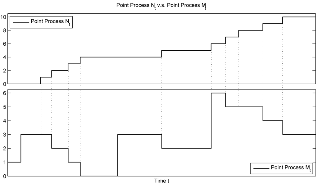
Figure 1. Point process $N_t$vs. Point process $M_t$.

Note that, the point process ${\left\{M_t\right\}}_{t\ge 0}$ is a non-negative process, as if $M_t=0$, there is no joint jump and $M_t$ cannot be brought downward further by one step or more; if $M_t=1,2,...$, $M_t$ is possible downward movement with a maximum of one step. The discrete piecewise non-negative process ${\left\{\delta M_t\right\}}_{t\ge 0}$, in fact, can be considered as the intensity process of the point process $N_t$ (proven later by Equation (4)).

3. Distributional Properties

The infinitesimal generator of a discretised dynamic contagion process $(M_t,N_t,t)$ acting on a function $f(m,n,t)\in \Omega \left(\mathcal{A}\right)$ is given by:

$$\begin{array}{ccc}\hfill \mathcal{A}f(m,n,t)& =& \frac{\partial f}{\partial t}+\rho \left(\sum _{k=0}^{\infty }f(m+k,n,t)p_k-f(m,n,t)\right)\hfill \end{array}$$

$$\begin{array}{ccc}& & +\delta m\left(\sum _{k=0}^{\infty }f(m+k-1,n+1,t)q_k-f(m,n,t)\right)\hfill \end{array}$$

(1)

where $\Omega \left(\mathcal{A}\right)$ is the domain of the generator $\mathcal{A}$, such that $f(m,n,t)$ is differentiable with respect to t, and for all m, n and t,

$$\begin{array}{ccc}\hfill \left|\sum _{k=0}^{\infty }f(m+k,n,t)p_k-f(m,n,t)\right|& <& \infty \hfill \\ \hfill \left|\sum _{k=0}^{\infty }f(m+k-1,n+1,t)q_k-f(m,n,t)\right|& <& \infty \hfill \end{array}$$

Following the methods adopted by Dassios and Embrechts [11] and later by Dassios and Jang [12] and Dassios and Zhao [8], we will use this generator Equation (1) with the aid of some properly selected martingales to find key distributional properties of $(N_t,M_t)$ as below.

3.1. Moments of $M_t$ and $N_t$

We derive the first moments of $M_t$ and $N_t$ by solving systems of ODEs and also discuss the stationarity condition for the process $M_t$.

Theorem 3.1. The expectation of $M_t$ conditional on $M_0$ is given by:

$$\mathbb{E}[M_t\mid M_0]=\left\{\begin{array}{cc}\frac{{\mu }_{1_P}\rho }{\kappa }+\left(M_0-\frac{{\mu }_{1_P}\rho }{\kappa }\right)e^{-\kappa t},\hfill & \kappa \ne 0\hfill \\ M_0+{\mu }_{1_P}\rho t,\hfill & \kappa =0\hfill \end{array}\right.$$

(2)

where $\kappa =\delta (1-{\mu }_{1_Q})$.

Proof. Set $f(m,n,t)=m$ and plug into generator Equation (1); we have:

$$\mathcal{A}m=\rho {\mu }_{1_P}+\delta m\left({\mu }_{1_Q}-1\right)$$

or $\mathcal{A}m=-\kappa m+{\mu }_{1_P}\rho$. Since $M_t-M_0-{\int }_0^t\mathcal{A}{M}_s\mathrm{d}s$ is a martingale, then,

$$\mathbb{E}\left[M_t\right|M_0]=M_0+\mathbb{E}\left[{\int }_0^t\mathcal{A}{M}_s\mathrm{d}s|M_0\right]=M_0-\kappa {\int }_0^t\mathbb{E}\left[M_s\right|M_0]\mathrm{d}s+{\mu }_{1_P}\rho t$$

and we can derive the expectation via the ODE:

$$\frac{\mathrm{d}u\left(t\right)}{\mathrm{d}t}=-\kappa u\left(t\right)+{\mu }_{1_P}\rho$$

where $u\left(t\right)=\mathbb{E}\left[M_t\right|M_0]$ with the initial condition: $u\left(0\right)=M_0$   □

Remark 3.2. The stationarity condition of process $M_t$ is:

$${\mu }_{1_Q}<1$$

(3)

Corollary 3.3. The expectation of $N_t$ conditional on $M_0$ is given by:

$$\mathbb{E}[N_t\mid M_0]=\left\{\begin{array}{cc}\frac{\delta }{\kappa }\left[{\mu }_{1_P}\rho t+\left(M_0-\frac{{\mu }_{1_P}\rho }{\kappa }\right)\left(1-e^{-\kappa t}\right)\right],\hfill & \kappa \ne 0\hfill \\ \delta \left(M_{0}t+\frac{1}{2}{\mu }_{1_P}\rho t^2\right),\hfill & \kappa =0\hfill \end{array}\right.$$

Proof. Set $f(m,n,t)=n$ and plug into generator Equation (1); we have $\mathcal{A}n=\delta m$. Since $N_t-N_0-{\int }_0^t\mathcal{A}{N}_s\mathrm{d}s$ is a martingale, then,

$$\mathbb{E}\left[N_t\right|M_0]=N_0+\mathbb{E}\left[{\int }_0^t\mathcal{A}{N}_s\mathrm{d}s|M_0\right]=\delta {\int }_0^t\mathbb{E}\left[M_s\right|M_0]\mathrm{d}s$$

(4)

where $\mathbb{E}\left[M_t\right|M_0]$ is given by Equation (2).   □

Higher moments of $M_t$ and $N_t$ can also be obtained similarly by this ODE method, and we omit them here.

3.2. Joint Probability Generating Function of $(M_T,N_T)$

Theorem 3.4. For constants $0\le \theta ,\phi \le 1$ and time $0\le t\le T$, we have the joint probability generating function of $(M_T,N_T)$,

$$\mathbb{E}\left[{\theta }^{(N_T-N_t)}{\phi }^{M_T}\mid {\mathcal{F}}_t\right]=e^{-\left(c\right(T)-c(t\left)\right)}{\left[A\left(t\right)\right]}^{M_t}$$

(5)

where $A\left(t\right)$ is determined by the non-linear ODE:

$$A^{\prime }\left(t\right)+\delta \theta \widehat{q}\left(A\left(t\right)\right)-\delta A\left(t\right)=0$$

with boundary condition $A\left(T\right)=\phi$; and $c\left(t\right)$ is determined by:

$$c\left(t\right)=\rho {\int }_0^t\left[1-\widehat{p}\left(A\left(s\right)\right)\right]\mathrm{d}s$$

Proof. Assume the exponential affine form:

$$f(m,n,t)={\left[A\left(t\right)\right]}^m{\theta }^n{e}^{c\left(t\right)}$$

and set $\mathcal{A}f(m,n,t)=0$ in generator Equation (1); then, we have:

$$\left\{\begin{array}{c}{A}^{\prime }\left(t\right)+\delta \theta \widehat{q}\left(A\left(t\right)\right)-\delta A\left(t\right)=0\hfill \\ c^{\prime }\left(t\right)=\rho [1-\widehat{p}\left(A\left(t\right)\right)]\hfill \end{array}\right.$$

Since ${\left[A\left(t\right)\right]}^{M_t}{\theta }^{N_t}{e}^{c\left(t\right)}$ is a martingale, we have:

$$\mathbb{E}\left[{\left[A\left(T\right)\right]}^{M_T}{\theta }^{N_T}{e}^{c\left(T\right)}|{\mathcal{F}}_t\right]={\left[A\left(t\right)\right]}^{M_t}{\theta }^{N_t}{e}^{c\left(t\right)}$$

with boundary conditions $A\left(T\right)=\phi$.   □

3.3. Probability Generating Function of $M_T$

Theorem 3.5. If ${\mu }_{1_Q}<1$, the probability generating function of $M_T$ conditional on $M_0$ is given by:

$$\mathbb{E}[{\phi }^{M_T}\mid M_0]=exp\left(-{\int }_{\phi }^{{\mathcal{Q}}_{\phi ,1}^{-1}\left(T\right)}\frac{\rho [1-\widehat{p}\left(u\right)]}{\delta \widehat{q}\left(u\right)-\delta u}\mathrm{d}u\right)\times {\left[{\mathcal{Q}}_{\phi ,1}^{-1}\left(T\right)\right]}^{M_0}$$

where:

$${\mathcal{Q}}_{\phi ,1}\left(L\right)=:{\int }_{\phi }^L\frac{\mathrm{d}u}{\delta \widehat{q}\left(u\right)-\delta u}$$

(6)

Proof. Set $t=0$, $\theta =1$ and assume $N_0=0$ in Theorem 3.4, and we have:

$$\mathbb{E}\left[{\phi }^{M_T}|M_0\right]=e^{-c\left(T\right)}{\left[A\left(0\right)\right]}^{M_0}$$

(7)

where $A\left(0\right)$ is uniquely determined by the non-linear ODE:

$$A^{\prime }\left(t\right)+\delta \widehat{q}\left(A\left(t\right)\right)-\delta A\left(t\right)=0$$

with boundary condition $A\left(T\right)=\phi$. Under the condition ${\mu }_{1_Q}<1$, it can be solved by the following steps:

• Set $A\left(t\right)=L(T-t)$ and $\tau =T-t$; this is equivalent to the initial value problem:

  $$\frac{\mathrm{d}L\left(\tau \right)}{\mathrm{d}\tau }=\delta \widehat{q}\left(L\left(\tau \right)\right)-\delta L\left(\tau \right)=:f_1\left(L\right)$$

  with initial condition $L\left(0\right)=\phi$; we define the right-hand side as the function $f_1\left(L\right)$.
• Since ${\mu }_{1_Q}<1$, we have:

  $$\begin{array}{c}\hfill \frac{\mathrm{d}{f}_1\left(L\right)}{\mathrm{d}L}=\delta \left(\sum _{k=0}^{\infty }k{L}^{k-1}{p}_k-1\right)\le \delta \left(\sum _{k=0}^{\infty }k{p}_k-1\right)=\delta \left({\mu }_{1_Q}-1\right)<0,0<L\le 1\end{array}$$

  then, $f_1\left(L\right)>0$ for $0<L<1$, since $f_1\left(1\right)=0$.
• Rewrite as:

  $$\frac{\mathrm{d}L}{\delta \widehat{q}\left(L\right)-\delta L}=\mathrm{d}\tau$$

  by integrating both sides from time zero to τ with initial condition $L\left(0\right)=\phi >0$; we have:

  $${\int }_{\phi }^L\frac{\mathrm{d}u}{\delta \widehat{q}\left(u\right)-\delta u}=\tau$$

  where $0<L\le 1$. We define the function on left-hand side as:

  $${\mathcal{Q}}_{\phi ,1}\left(L\right)=:{\int }_{\phi }^L\frac{\mathrm{d}u}{\delta \widehat{q}\left(u\right)-\delta u}$$

  then, ${\mathcal{Q}}_{\phi ,1}\left(L\right)=\tau$. Obviously, $L\to \phi$ when $\tau \to 0$; by convergence test,

  $$\begin{array}{c}\hfill \underset{u\to 1}{lim}\frac{\frac{1}{1-u}}{\frac{1}{\delta \widehat{q}\left(u\right)-\delta u}}=\delta \underset{u\to 1}{lim}\frac{\widehat{q}\left(u\right)-u}{1-u}=\delta \underset{u\to 1}{lim}\frac{{\left(\widehat{q}\left(u\right)-u\right)}^{\prime }}{{(1-u)}^{\prime }}=1-{\mu }_{1_Q}>0\end{array}$$

  and we know that ${\int }_{\phi }^1\frac{1}{1-u}\mathrm{d}u=\infty$; then,

  $${\int }_{\phi }^1\frac{\mathrm{d}u}{\delta \widehat{q}\left(u\right)-\delta u}=\infty$$

  Hence, $L\to 1$ when $\tau \to \infty$; the integrand is positive in the domain $u\in [\phi ,1)$ and also ${\mathcal{Q}}_{\phi ,1}\left(L\right)$ is a strictly increasing function; therefore, ${\mathcal{Q}}_{\phi ,1}\left(L\right):[\phi ,1)\to [0,\infty )$ is a well-defined (monotone) function, and its inverse function ${\mathcal{Q}}_{\phi ,1}^{-1}\left(\tau \right):[0,\infty )\to [\phi ,1)$ exists.
• The unique solution is found by:

  $$L\left(\tau \right)={\mathcal{Q}}_{\phi ,1}^{-1}\left(\tau \right),\mathrm{or},A\left(t\right)={\mathcal{Q}}_{\phi ,1}^{-1}(T-t)$$
• $A\left(0\right)$ is obtained,

  $$A\left(0\right)=L\left(T\right)={\mathcal{Q}}_{\phi ,1}^{-1}\left(T\right)$$

Then, $c\left(T\right)$ is determined by:

$$c\left(T\right)=\rho {\int }_0^T\left[1-\widehat{p}\left({\mathcal{Q}}_{\phi ,1}^{-1}\left(\tau \right)\right)\right]\mathrm{d}\tau$$

by the change of variable ${\mathcal{Q}}_{\phi ,1}^{-1}\left(\tau \right)=u$; we have $\tau ={\mathcal{Q}}_{\phi ,1}\left(u\right)$, and:

$${\int }_0^T\left[1-\widehat{h}\left({\mathcal{Q}}_{\phi ,1}^{-1}\left(\tau \right)\right)\right]\mathrm{d}\tau ={\int }_{{\mathcal{Q}}_{\phi ,1}^{-1}\left(0\right)}^{{\mathcal{Q}}_{\phi ,1}^{-1}\left(T\right)}[1-\widehat{p}\left(u\right)]\frac{\partial \tau }{\partial u}\mathrm{d}u={\int }_{\phi }^{{\mathcal{Q}}_{\phi ,1}^{-1}\left(T\right)}\frac{1-\widehat{p}\left(u\right)}{\delta \widehat{q}\left(u\right)-\delta u}\mathrm{d}u$$

   □

Theorem 3.6. If ${\mu }_{1_Q}<1$, the probability generating function of the asymptotic distribution of $M_T$ is given by:

$$\underset{T\to \infty }{lim}\mathbb{E}[{\phi }^{M_T}\mid M_0]=exp\left(-{\int }_{\phi }^1\frac{\rho [1-\widehat{p}\left(u\right)]}{\delta \widehat{q}\left(u\right)-\delta u}\mathrm{d}u\right)$$

(8)

and this is also the probability generating function of the stationary distribution of process ${\left\{M_t\right\}}_{t\ge 0}$.

Proof. Since ${lim}_{T\to \infty }{\mathcal{Q}}_{\phi ,1}^{-1}\left(T\right)=1$, and by Theorem 3.5, we have the probability generating function of the asymptotic distribution of $M_T$ immediately.

To further prove the stationarity, by Proposition 9.2 of Ethier and Kurtz [13], we need to prove that, for any function $f\in \Omega \left(\mathcal{A}\right)$, we have:

$$\sum _{m=0}^{\infty }\mathcal{A}f\left(m\right){\aleph }_m=0$$

(9)

where $\mathcal{A}f\left(m\right)$ is the infinitesimal generator of the discretised dynamic contagion process acting on $f\left(m\right)$, i.e.,

$$\mathcal{A}f\left(m\right)=\rho \left(\sum _{k=0}^{\infty }f(m+k)p_k-f\left(m\right)\right)+\delta m\left(\sum _{k=0}^{\infty }f(m+k-1)q_k-f\left(m\right)\right)$$

(10)

and ${\left\{{\aleph }_m\right\}}_{k=0,1,2,...}$ are the probabilities of m with the probability generating function given by Equation (8). Now, we try to solve Equation (9).

For the first term of Equation (9), we have:

$$\begin{array}{ccc}& & \sum _{m=0}^{\infty }\left[\rho \left(\sum _{k=0}^{\infty }f(m+k)p_k\right)\right]{\aleph }_m\hfill \\ & =& \rho \sum _{m=0}^{\infty }{\aleph }_m\sum _{k=0}^{\infty }f(m+k)p_k(j=m+k)\hfill \\ & =& \rho \sum _{j=0}^{\infty }f\left(j\right)\sum _{k=0}^j{\aleph }_{j-k}{p}_k\hfill \\ & =& \rho \sum _{m=0}^{\infty }f\left(m\right)\sum _{k=0}^m{\aleph }_{m-k}{p}_k\hfill \end{array}$$

For the second term of Equation (9), we have:

$$\begin{array}{ccc}& & \sum _{m=0}^{\infty }\left[\delta m\left(\sum _{k=0}^{\infty }f(m+k-1)q_k\right)\right]{\aleph }_m\hfill \\ & =& \delta \sum _{m=0}^{\infty }m{\aleph }_m\sum _{k=0}^{\infty }f(m+k-1)q_k\hfill \\ & =& \delta \sum _{m=-1}^{\infty }(m+1){\aleph }_{m+1}\sum _{k=0}^{\infty }f(m+k)q_k\hfill \\ & =& \delta \sum _{m=0}^{\infty }(m+1){\aleph }_{m+1}\sum _{k=0}^{\infty }f(m+k)q_k(j=m+k)\hfill \\ & =& \delta \sum _{j=0}^{\infty }f\left(j\right)\sum _{k=0}^j(j-k+1){\aleph }_{j-k+1}{q}_k\hfill \\ & =& \delta \sum _{m=0}^{\infty }f\left(m\right)\sum _{k=0}^m(m-k+1){\aleph }_{m-k+1}{q}_k\hfill \end{array}$$

Therefore,

$$\begin{array}{ccc}& & \sum _{m=0}^{\infty }\mathcal{A}f\left(m\right){\aleph }_m\hfill \\ & =& \sum _{m=0}^{\infty }f\left(m\right)\left[\rho \left(\sum _{k=0}^m{\aleph }_{m-k}{p}_k-{\aleph }_m\right)+\delta \left(\sum _{k=0}^m(m-k+1){\aleph }_{m-k+1}{q}_k-m{\aleph }_m\right)\right]\hfill \\ & =& 0\hfill \end{array}$$

for any function $f\left(m\right)\in \Omega \left(\mathcal{A}\right)$; then, we have recursive equation:

$$\begin{array}{c}\hfill \rho \left(\sum _{k=0}^m{\aleph }_{m-k}{p}_k-{\aleph }_m\right)+\delta \left(\sum _{k=0}^m(m-k+1){\aleph }_{m-k+1}{q}_k-m{\aleph }_m\right)=0\end{array}$$

and:

$$\begin{array}{c}\hfill \sum _{m=0}^{\infty }{\phi }^m\times \left[\rho \left(\sum _{k=0}^m{\aleph }_{m-k}{p}_k-{\aleph }_m\right)+\delta \left(\sum _{k=0}^m(m-k+1){\aleph }_{m-k+1}{q}_k-m{\aleph }_m\right)\right]=0\end{array}$$

By the Laplace transform:

$$\widehat{\aleph }\left(\phi \right)=:\mathcal{L}\left\{{\aleph }_m\right\}=\sum _{m=0}^{\infty }{\aleph }_m{\phi }^m$$

since:

$$\begin{array}{ccc}& & \sum _{m=0}^{\infty }{\phi }^m\sum _{k=0}^m{\aleph }_{m-k}{p}_k\hfill \\ & =& \sum _{k=0}^{\infty }\sum _{m=k}^{\infty }{\phi }^{m-k}{\aleph }_{m-k}{\phi }^k{p}_k\left(\sum _{m=k}^{\infty }{\phi }^{m-k}{\aleph }_{m-k}=\widehat{\aleph }\left(\phi \right)\right)\hfill \\ & =& \widehat{\aleph }\left(\phi \right)\widehat{p}\left(\phi \right)\hfill \end{array}$$

$$\begin{array}{ccc}& & \sum _{m=0}^{\infty }{\phi }^m\sum _{k=0}^m(m-k+1){\aleph }_{m-k+1}{q}_k\hfill \\ & =& \sum _{m=0}^{\infty }{\phi }^m\sum _{j=1}^{m+1}j{\aleph }_j{q}_{m+1-j}(j=m-k+1)\hfill \\ & =& \frac{1}{\phi }\sum _{m=0}^{\infty }{\phi }^j\sum _{j=1}^{m+1}j{\aleph }_j{q}_{m+1-j}{\phi }^{m+1-j}(i=m+1)\hfill \\ & =& \frac{1}{\phi }\sum _{j=1}^{\infty }\sum _{i=j}^{\infty }{q}_{i-j}{\phi }^{i-j}{\phi }^{j}j{\aleph }_j\left(\sum _{i=j}^{\infty }{q}_{i-j}{\phi }^{i-j}=\widehat{q}\left(\phi \right)\right)\hfill \\ & =& \widehat{q}\left(\phi \right)\sum _{j=0}^{\infty }j{\phi }^{j-1}{\aleph }_j\hfill \\ & =& \widehat{q}\left(\phi \right){\widehat{\aleph }}^{\prime }\left(\phi \right)\hfill \end{array}$$

and:

$$\sum _{m=0}^{\infty }{\phi }^{m}m{\aleph }_m=\phi \sum _{m=0}^{\infty }m{\aleph }_m{\phi }^{m-1}=\phi {\widehat{\aleph }}^{\prime }\left(\phi \right)$$

we have the ODE of $\widehat{\aleph }\left(\phi \right)$,

$$\rho \left(\widehat{\aleph }\left(\phi \right)\widehat{p}\left(\phi \right)-\widehat{\aleph }\left(\phi \right)\right)+\delta \left(\widehat{q}\left(\phi \right){\widehat{\aleph }}^{\prime }\left(\phi \right)-\phi {\widehat{\aleph }}^{\prime }\left(\phi \right)\right)=0$$

then,

$$\widehat{\aleph }\left(\phi \right)=\widehat{\aleph }\left(1\right)exp\left(-{\int }_{\phi }^1\frac{\rho [1-\widehat{p}\left(u\right)]}{\delta \widehat{q}\left(u\right)-\delta u}\mathrm{d}u\right)$$

with the initial condition $\widehat{\aleph }\left(1\right)=1$; hence, we have the unique solution:

$$\widehat{\aleph }\left(\phi \right)=exp\left(-{\int }_{\phi }^1\frac{\rho [1-\widehat{p}\left(u\right)]}{\delta \widehat{q}\left(u\right)-\delta u}\mathrm{d}u\right)$$

which is exactly given by Equation (8).

Since the distribution ℵ is the unique solution to Equation (9), we have the stationarity for the process ${\left\{M_t\right\}}_{t\ge 0}$.   □

Remark 3.7. If ${\mu }_{1_Q}<1$, $M_0\sim \aleph$, then $M_T\sim \aleph$, since by Theorem 3.6 and Theorem 3.5, we have:

$$\begin{array}{ccc}& & \mathbb{E}\left[{\psi }^{M_T}\right]\hfill \\ & =& \mathbb{E}\left[\left[{\psi }^{M_T}|M_0\right]\right]\hfill \\ & =& exp\left(-{\int }_{\phi }^{{\mathcal{Q}}_{\phi ,1}^{-1}\left(T\right)}\frac{\rho [1-\widehat{p}\left(u\right)]}{\delta \widehat{q}\left(u\right)-\delta u}\mathrm{d}u\right)\times \mathbb{E}\left[{\left[{\mathcal{Q}}_{\phi ,1}^{-1}\left(T\right)\right]}^{M_0}\right]\hfill \\ & =& exp\left(-{\int }_{\phi }^{{\mathcal{Q}}_{\phi ,1}^{-1}\left(T\right)}\frac{\rho [1-\widehat{p}\left(u\right)]}{\delta \widehat{q}\left(u\right)-\delta u}\mathrm{d}u\right)\times exp\left(-{\int }_{{\mathcal{Q}}_{\phi ,1}^{-1}\left(T\right)}^1\frac{\rho [1-\widehat{p}\left(u\right)]}{\delta \widehat{q}\left(u\right)-\delta u}\mathrm{d}u\right)\hfill \\ & =& \widehat{\aleph }\left(\phi \right)\hfill \end{array}$$

which also reflects the stationarity of process ${\left\{M_t\right\}}_{t\ge 0}$.

3.4. Probability Generating Function of $N_T$

Theorem 3.8. Suppose ${\mu }_{1_Q}<1$ and $N_0=0$; the probability generating function of $N_T$ conditional on $M_0$ is given by:

$$\mathbb{E}\left[{\theta }^{N_T}\mid M_0\right]=exp\left(-{\int }_{{\mathcal{Q}}_{0,\theta }^{-1}\left(T\right)}^1\frac{\rho [1-\widehat{p}\left(u\right)]}{\delta u-\delta \theta \widehat{q}\left(u\right)}\mathrm{d}u\right)\times {\left[{\mathcal{Q}}_{0,\theta }^{-1}\left(T\right)\right]}^{M_0}$$

where:

$${\mathcal{Q}}_{0,\theta }\left(L\right)=:{\int }_L^1\frac{\mathrm{d}u}{\delta u-\delta \theta \widehat{q}\left(u\right)},0\le \theta <1$$

(11)

Proof. By setting $t=0$, $\phi =1$ and assuming $N_0=0$ in Theorem 3.4, we have:

$$\mathbb{E}\left[{\theta }^{N_T}\mid M_0\right]=e^{-c\left(T\right)}{\left[A\left(0\right)\right]}^{M_0}$$

(12)

where $A\left(0\right)$ is uniquely determined by the non-linear ODE:

$$A^{\prime }\left(t\right)+\delta \theta \widehat{q}\left(A\left(t\right)\right)-\delta A\left(t\right)=0$$

with boundary condition $A\left(T\right)=1$. It can be solved, under the condition ${\mu }_{1_Q}<1$, by the following steps:

• Set $A\left(t\right)=L(T-t)$ and $\tau =T-t$,

  $$\frac{\mathrm{d}L\left(\tau \right)}{\mathrm{d}\tau }=\delta \theta \widehat{q}\left(L\left(\tau \right)\right)-\delta L\left(\tau \right)=:f_2\left(L\right),0\le \theta <1$$

  (13)

  with initial condition $L\left(0\right)=1$; we define the right-hand side as the function $f_2\left(L\right)$.
• There is only one positive singular point in the interval $[0,1]$, denoted by:

  $$0\le {\phi }^{*}\le 1$$

  (14)

  by solving the equation $f_2\left(L\right)=0$. This is because, for the case $0<\theta <1$, the equation $f_2\left(L\right)=0$ is equivalent to:

  $$\widehat{q}\left(u\right)=\frac{1}{\theta }u,0<\theta <1$$

  note that $\widehat{q}(·)$ is a convex function, then it is clear that there is only one positive solution within $[0,1]$ to this equation; in particularly when $\theta \to 0$, ${\phi }^{*}\to 0$. Then, we have $f_2\left(L\right)<0$ for ${\phi }^{*}<L\le 1$.
• Rewrite Equation (13) as:

  $$\frac{\mathrm{d}L}{\delta L-\delta \theta \widehat{q}\left(L\right)}=-\mathrm{d}\tau$$

  and integrate,

  $${\int }_L^1\frac{\mathrm{d}u}{\delta u-\delta \theta \widehat{q}\left(u\right)}=\tau$$

  where ${\phi }^{*}<L\le 1$; we define the function on left-hand side as:

  $${\mathcal{Q}}_{0,\theta }\left(L\right)=:{\int }_L^1\frac{\mathrm{d}u}{\delta u-\delta \theta \widehat{q}\left(u\right)}$$

  then, ${\mathcal{Q}}_{0,\theta }\left(L\right)=\tau$, as $L\to 1$ when $\tau \to 0$ and $L\to {\phi }^{*}$ when $\tau \to \infty$; the integrand is positive in the domain $u\in ({\phi }^{*},1]$ and $L\ge 0$, ${\mathcal{Q}}_{0,\theta }\left(L\right)$ is a strictly decreasing function. Therefore, ${\mathcal{Q}}_{0,\theta }\left(L\right):({\phi }^{*},1]\to [0,\infty )$ is a well-defined function, and its inverse function ${\mathcal{Q}}_{0,\theta }^{-1}\left(\tau \right):[0,\infty )\to ({\phi }^{*},1]$ exists.
• The unique solution is found by $L\left(\tau \right)={\mathcal{Q}}_{0,\theta }^{-1}\left(\tau \right)$, or, $A\left(t\right)={\mathcal{Q}}_{0,\theta }^{-1}(T-t)$.
• $A\left(0\right)$ is obtained,

  $$A\left(0\right)=L\left(T\right)={\mathcal{Q}}_{0,\theta }^{-1}\left(T\right)$$

Then, $c\left(T\right)$ is determined by:

$$c\left(T\right)=\rho {\int }_0^T\left[1-\widehat{p}\left({\mathcal{Q}}_{0,\theta }^{-1}\left(\tau \right)\right)\right]\mathrm{d}\tau$$

where, by the change of variable,

$${\int }_0^T\left[1-\widehat{p}\left({\mathcal{Q}}_{0,\theta }^{-1}\left(\tau \right)\right)\right]\mathrm{d}\tau ={\int }_{{\mathcal{Q}}_{0,\theta }^{-1}\left(T\right)}^1\frac{1-\widehat{p}\left(u\right)}{\delta u-\delta \theta \widehat{q}\left(u\right)}\mathrm{d}u$$

   □

4. Special Cases

In this section, we focus on three important special cases where more explicit results for the distributional properties of the numbers of settled and unsettled claims ${\left\{\left(N_t,M_t\right)\right\}}_{t\ge 0}$ can be derived, and the associated numerical examples are also provided.

4.1. Case $p_1=1$

Case $p_1=1$ is defined as the special case of a discretised dynamic contagion process when:

$$p_1=1,{\left\{p_k\right\}}_{k\ne 1}=0;q_0=1,{\left\{q_k\right\}}_{k\ne 0}=0$$

(15)

This simple case could be applied, for instance, to model the delaying arrival of claims in the ruin problem for an insurance company; see more details in Dassios and Zhao [9].

Theorem 4.1. For any time $t_2>t_1\ge 0$, if $M_{t_1}\sim \mathrm{Poisson}\left(\upsilon \right)$, $\upsilon \ge 0$, then,

$$\begin{array}{ccc}\hfill M_{t_2}& \sim & \mathrm{Poisson}\left(\upsilon e^{-\delta (t_2-t_1)}+\rho \frac{1-e^{-\delta (t_2-t_1)}}{\delta }\right)\hfill \\ \hfill N_{t_2}-N_{t_1}& \sim & \mathrm{Poisson}\left(\upsilon \left(1-e^{-\delta (t_2-t_1)}\right)+\rho \left((t_2-t_1)-\frac{1-e^{-\delta (t_2-t_1)}}{\delta }\right)\right)\hfill \end{array}$$

and they are independent.

Proof. By setting $T=t_2,t=t_1$ in Theorem 3.4, we have:

$$\mathbb{E}\left[{\phi }^{M_{t_2}}{\theta }^{N_{t_2}-N_{t_1}}\mid M_{t_1}\right]={\left[A\left(t_1\right)\right]}^{M_{t_1}}{e}^{-\left(c\left(t_2\right)-c\left(t_1\right)\right)}$$

where $A\left(t\right)$ and $c\left(t\right)$ can be solved explicitly as:

$$\begin{array}{ccc}\hfill A\left(t\right)& =& (\phi -\theta )e^{-\delta (t_2-t)}+\theta ,\hfill \\ \hfill c\left(t_2\right)-c\left(t_1\right)& =& \rho \left((1-\theta )(t_2-t_1)-(\phi -\theta )\frac{1-e^{-\delta (t_2-t_1)}}{\delta }\right)\hfill \end{array}$$

The joint probability generating function of $M_{t_2}$ and $N_{t_2}-N_{t_1}$ is given by:

$$\begin{array}{ccc}& & \mathbb{E}\left[{\phi }^{M_{t_2}}{\theta }^{N_{t_2}-N_{t_1}}\right]\hfill \\ & =& \mathbb{E}\left[\mathbb{E}\left[{\phi }^{M_{t_2}}{\theta }^{N_{t_2}-N_{t_1}}\mid M_{t_1}\right]\right]\hfill \\ & =& \mathbb{E}\left[{\left[A\left(t_1\right)\right]}^{M_{t_1}}\right]e^{-\left(c\left(t_2\right)-c\left(t_1\right)\right)}\hfill \\ & =& e^{-\upsilon \left(1-A\left(t_1\right)\right)}{e}^{-\left(c\left(t_2\right)-c\left(t_1\right)\right)}\hfill \\ & =& exp\left(-\upsilon \left[(1-\theta )-(\phi -\theta )e^{-\delta (t_2-t_1)}\right]-\rho \left[(1-\theta )(t_2-t_1)-(\phi -\theta )\frac{1-e^{-\delta (t_2-t_1)}}{\delta }\right]\right)\hfill \end{array}$$

Set $\theta =1$ and $\phi =1$, respectively; we have Poisson marginal distributions of $M_{t_2}$ and $N_{t_2}-N_{t_1}$, since:

$$\begin{array}{ccc}\hfill \mathbb{E}\left[{\phi }^{M_{t_2}}\right]& =& exp\left(-(1-\phi )\left[\upsilon e^{-\delta (t_2-t_1)}+\rho \frac{1-e^{-\delta (t_2-t_1)}}{\delta }\right]\right),\hfill \end{array}$$

$$\begin{array}{ccc}\hfill \mathbb{E}\left[{\theta }^{N_{t_2}-N_{t_1}}\right]& =& exp\left(-(1-\theta )\left[\upsilon \left(1-e^{-\delta (t_2-t_1)}\right)+\rho \left((t_2-t_1)-\frac{1-e^{-\delta (t_2-t_1)}}{\delta }\right)\right]\right)\hfill \end{array}$$

(16)

Obviously, they are also independent as:

$$\mathbb{E}\left[{\phi }^{M_{t_2}}\times {\theta }^{N_{t_2}-N_{t_1}}\right]=\mathbb{E}\left[{\phi }^{M_{t_2}}\right]\times \mathbb{E}\left[{\theta }^{N_{t_2}-N_{t_1}}\right]$$

   □

Corollary 4.2. If $M_0\sim \mathrm{Poisson}\left(\zeta \right)$, $\zeta \ge 0$, then:

$$\begin{array}{ccc}\hfill M_t& \sim & \mathrm{Poisson}\left(\zeta e^{-\delta t}+\rho \frac{1-e^{-\delta t}}{\delta }\right)\hfill \\ \hfill N_t& \sim & \mathrm{Poisson}\left(\zeta \left(1-e^{-\delta t}\right)+\rho \left(t-\frac{1-e^{-\delta t}}{\delta }\right)\right)\hfill \end{array}$$

and they are independent.

Proof. Set $t_1=0$, $t_2=t>0$ and $\upsilon =\zeta$ in Theorem 4.1; the results follow immediately.   □

Corollary 4.3. If $M_0\sim \mathrm{Poisson}\left(\zeta \right)$, then $N_t$ is a non-homogeneous Poisson process of rate $\rho +\left(\zeta \delta -\rho \right)e^{-\delta t}$.

Proof. For any time $t_2>t_1\ge 0$, by Corollary 4.2, we have:

$$M_{t_1}\sim \mathrm{Poisson}\left(\zeta e^{-\delta t_1}+\rho \frac{1-e^{-\delta t_1}}{\delta }\right)$$

By Theorem 4.1, set $\upsilon =\zeta e^{-\delta t_1}+\rho \frac{1-e^{-\delta t_1}}{\delta }$ in Equation (16), then,

$$\mathbb{E}\left[{\theta }^{N_{t_2}-N_{t_1}}\right]=exp\left(-(1-\theta ){\int }_{t_1}^{t_2}\left[\zeta \delta e^{-\delta s}+\rho \left(1-e^{-\delta s}\right)\right]\mathrm{d}s\right)$$

hence, the increments of $N_t$ follow a Poisson distribution,

$$N_{t_2}-N_{t_1}\sim \mathrm{Poisson}\left({\int }_{t_1}^{t_2}\left[\zeta \delta e^{-\delta s}+\rho \left(1-e^{-\delta s}\right)\right]\mathrm{d}s\right)$$

Based on Theorem 4.1 and Corollary 4.2, we observe that $M_{t_2}$ and $N_{t_2}-N_{t_1}$ are both Poisson distributed and independent. Because of the Markov property, all of the future increments after $N_{t_2}$ only depend on $M_{t_2}$; they are independent of $N_{t_2}-N_{t_1}$, as well, i.e., for any random variable $X\in \sigma \left\{{\mathcal{N}}_s:N_s-N_{t_2},s\ge t_2\right\}$, we have:

$$\begin{array}{ccc}\hfill \mathbb{E}\left[X{\theta }^{N_{t_2}-N_{t_1}}\right]& =& \mathbb{E}\left[\mathbb{E}\left[X{\theta }^{N_{t_2}-N_{t_1}}|M_{t_2}\right]\right]\hfill \\ & =& \mathbb{E}\left[\mathbb{E}\left[X|M_{t_2}\right]\times \mathbb{E}\left[{\theta }^{N_{t_2}-N_{t_1}}|M_{t_2}\right]\right]\hfill \\ & =& \mathbb{E}\left[\mathbb{E}\left[X|M_{t_2}\right]\right]\times \mathbb{E}\left[\mathbb{E}\left[{\theta }^{N_{t_2}-N_{t_1}}|M_{t_2}\right]\right]\hfill \\ & =& \mathbb{E}\left[X\right]{\theta }^{N_{t_2}-N_{t_1}}\hfill \end{array}$$

The increments of the point process $N_t$ follow a Poisson distribution and also they are independent; therefore, $N_t$ is a non-homogeneous Poisson process of rate $\zeta \delta e^{-\delta t}+\rho \left(1-e^{-\delta t}\right)$.   □

In particular, if and only if $\zeta =\frac{\rho }{\delta }$, $N_t$ is a Poisson process with a rate of ρ. Corollary 4.3, in fact, recovers the result obtained earlier by Mirasol [14], i.e., a delayed (or displaced) Poisson process is still a (non-homogeneous) Poisson process; see also Newell [15] and Lawrance and Lewis [16].

4.2. Case $q_1=q$

Case $q_1=q$ is defined as the special case of a discretised dynamic contagion process when:

$$p_1=1,{\left\{p_k\right\}}_{k\ne 1}=0;q_0=1-q,q_1=q,{\left\{q_k\right\}}_{k=2,3,...}=0;0\le q<1$$

(17)

Corollary 4.4. The stationary distribution of $M_t$ is a Poisson distribution specified by:

$${\left\{M_t\right\}}_{t\ge 0}\sim \mathrm{Poisson}\left(\frac{\rho }{\delta (1-q)}\right)$$

Proof. The stationarity condition holds as ${\mu }_{1_Q}=q<1$; then, by Theorem 3.6, we have:

$$\widehat{\aleph }\left(\phi \right)=e^{-\frac{\rho }{\delta (1-q)}(1-\phi )}$$

which is the probability generating function of a Poisson distribution with constant intensity $\frac{\rho }{\delta (1-q)}$.   □

Corollary 4.5 The probability generating function of $N_T$ is given by:

$$\mathbb{E}\left[{\theta }^{N_T}\mid M_0\right]=exp\left(-\frac{\rho }{\delta }\frac{1-\theta }{1-\theta q}\left[\delta T-\frac{1-e^{-(1-\theta q)\delta T}}{1-\theta q}\right]\right){\left[\frac{\theta (1-q)+(1-\theta )e^{-(1-\theta q)\delta T}}{1-\theta q}\right]}^{M_0}$$

(18)

if $M_0\sim \mathrm{Poisson}\left(\frac{\rho }{\delta (1-q)}\right)$, then,

$$\mathbb{E}\left[{\theta }^{N_T}\right]=exp\left(-\rho T\left(1-\frac{1-q}{1-\theta q}\theta \right)\right)exp\left(-\frac{\rho }{\delta }\frac{q}{1-q}{\left(1-\frac{1-q}{1-\theta q}\theta \right)}^2\left(1-e^{-(1-\theta q)\delta T}\right)\right)$$

(19)

Proof. The stationarity condition holds as ${\mu }_{1_Q}=q<1$. By Theorem 3.8, the results follow, since:

$${\mathcal{Q}}_{0,\theta }^{-1}\left(T\right)=\frac{\theta (1-q)+(1-\theta )e^{-(1-\theta q)\delta T}}{1-\theta q},0\le \theta <1$$

   □

Note that the first term of $\mathbb{E}\left[{\theta }^{N_T}\right]$ of Equation (19) is the probability generating function of a compound Poisson distribution $N_1$ with point ${\stackrel{°}{N}}_T\sim \mathrm{Poisson}\left(\rho T\right)$ and underlying $X_1\sim \mathrm{Geometric}(1-q)$ where:

$$P\{X_1=j\}=q^{j-1}(1-q),j=1,2,...,\mathbb{E}\left[{\theta }^{X_1}\right]=\frac{1-q}{1-\theta q}\theta$$

The second term is the the probability generating function of a proper random variable $\tilde{O}$. Hence, $N_T=N_1+\tilde{O}$, and $N_T$ is stochastically larger than $N_1$, i.e., $N_T\succ N_1$.

Given the probability generating function of $N_T$ in Corollary 4.5, the probability distribution of the number of the cumulative settled claims at time T can be obtained explicitly by the basic property:

$$P\{N_T=n\mid M_0\}=\frac{\partial n}{\partial {\theta }^n}\mathbb{E}\left[{\theta }^{N_T}\mid M_0\right]{|}_{\theta =0}$$

Numerical examples with the specified parameters $(\rho ,\delta ,q)=(1,1,0.5)$ are provided in Table 1.

Table 1. Numerical examples for case $q_1=q$ based on Corollary 4.5: the probability distribution of the number of cumulative settled claims at time T with parameters $(\rho ,\delta ,q)=(1,1,0.5)$.

	$P\{N_T=n|M_0=0\}$ (%)			$P\{N_T=n|M_0=5\}$ (%)
n	$T=1$	$T=2$	$T=5$	$T=1$	$T=2$	$T=5$
0	69.2201	32.1314	1.8193	0.4664	0.0015	0.0000
1	21.8777	27.7829	4.5175	3.3169	0.0319	0.0000
2	6.6404	18.9572	7.3929	10.3724	0.2956	0.0000
3	1.7365	10.9172	9.7336	18.9468	1.5260	0.0001
4	0.4113	5.6055	11.1254	22.8201	4.8543	0.0047
5	0.0906	2.6432	11.4776	19.6109	10.1416	0.0852
6	0.0188	1.1655	10.9392	12.8517	14.9512	0.3778
7	0.0037	0.4865	9.7807	6.8021	17.0146	1.0198
8	0.0007	0.1939	8.2921	3.0379	15.9371	2.0730
9	0.0001	0.0742	6.7191	1.1825	12.8316	3.4803
10	0.0000	0.0275	5.2352	0.4109	9.1512	5.0745
Sum	100.0000	99.9850	87.0325	99.8186	86.7366	12.1154

Table 1. Numerical examples for case $q_1=q$ based on Corollary 4.5: the probability distribution of the number of cumulative settled claims at time T with parameters $(\rho ,\delta ,q)=(1,1,0.5)$.

	$P\{N_T=n|M_0=0\}$ (%)			$P\{N_T=n|M_0=5\}$ (%)
n	$T=1$	$T=2$	$T=5$	$T=1$	$T=2$	$T=5$
0	69.2201	32.1314	1.8193	0.4664	0.0015	0.0000
1	21.8777	27.7829	4.5175	3.3169	0.0319	0.0000
2	6.6404	18.9572	7.3929	10.3724	0.2956	0.0000
3	1.7365	10.9172	9.7336	18.9468	1.5260	0.0001
4	0.4113	5.6055	11.1254	22.8201	4.8543	0.0047
5	0.0906	2.6432	11.4776	19.6109	10.1416	0.0852
6	0.0188	1.1655	10.9392	12.8517	14.9512	0.3778
7	0.0037	0.4865	9.7807	6.8021	17.0146	1.0198
8	0.0007	0.1939	8.2921	3.0379	15.9371	2.0730
9	0.0001	0.0742	6.7191	1.1825	12.8316	3.4803
10	0.0000	0.0275	5.2352	0.4109	9.1512	5.0745
Sum	100.0000	99.9850	87.0325	99.8186	86.7366	12.1154

4.3. Case $q_0=1$

Case $q_0=1$ is defined as the special case of a discretised dynamic contagion process when:

$$q_0=1,{\left\{q_k\right\}}_{k\ne 0}=0$$

(20)

Indeed, this is a special case which corresponds to a Cox process with shot-noise intensity via transformation, as given by Appendix A.

Corollary 4.6. If ${\left\{p_k\right\}}_{k=0,1,2,...}\sim \mathrm{Geometric}\left(p\right)$, $0\le p<1$, then, the stationary distribution of $M_t$ is given:

$${\left\{M_t\right\}}_{t\ge 0}\sim \mathrm{NegBin}\left(\frac{\rho }{\delta },1-p\right)$$

Proof. If ${\left\{p_k\right\}}_{k=0,1,2,...}\sim \mathrm{Geometric}\left(p\right)$, then,

$$\widehat{p}\left(u\right)=\frac{p}{1-(1-p)u}$$

(21)

The stationarity condition holds as ${\mu }_{1_Q}=0<1$; then, by Theorem 3.6, we have:

$$\widehat{\aleph }\left(\phi \right)={\left(\frac{p}{1-(1-p)\phi }\right)}^{\frac{\rho }{\delta }}$$

which is the probability generating function of a negative binomial distribution with the parameters $\left(\frac{\rho }{\delta },1-p\right)$.   □

Corollary 4.7. If ${\left\{p_k\right\}}_{k=0,1,2,...}\sim \mathrm{Geometric}\left(p\right)$, then,

$$\mathbb{E}\left[{\theta }^{N_T}\mid M_0\right]=e^{-\rho T\left(1-\widehat{p}\left(\theta \right)\right)}{\left(\frac{p_T}{1-\left(1-p_T\theta \right)}\right)}^{-\frac{\rho }{\delta }\widehat{p}\left(\theta \right)}{\left[(1-\theta )e^{-\delta T}+\theta \right]}^{M_0}$$

where $\widehat{p}\left(u\right)$ is specified by Equation (21) and

$$p_T=:\frac{p}{1-(1-p)e^{-\delta T}}$$

if $M_0\sim \mathrm{NegBin}\left(\frac{\rho }{\delta },1-p\right)$, then,

$$\mathbb{E}\left[{\theta }^{N_T}\right]=e^{-\rho T\left(1-\widehat{p}\left(\theta \right)\right)}{\left(\frac{p_T}{1-\left(1-p_T\theta \right)}\right)}^{\frac{\rho }{\delta }\left(1-\widehat{p}\left(\theta \right)\right)}$$

(22)

Proof. By Theorem 3.8, the results follow, since:

$${\mathcal{Q}}_{0,\theta }^{-1}\left(T\right)=(1-\theta )e^{-\delta T}+\theta ,0\le \theta <1$$

(23)

   □

Note that the first term of $\mathbb{E}\left[{\theta }^{N_T}\right]$ of Equation (22) is the probability generating function of a compound Poisson distribution $N_2$ with point ${\stackrel{°}{N}}_T\sim \mathrm{Poisson}\left(\rho T\right)$ and underlying $X_2\sim \mathrm{Geometric}\left(p\right)$, where:

$$P\{X_2=j\}={(1-p)}^{j}p,j=0,1,2,...,\mathbb{E}\left[{\theta }^{X_2}\right]=\frac{p}{1-(1-p)\theta }$$

the second term of Equation (22) is the probability generating function of a proper random variable $\tilde{O}$. Hence, we have $N_T=N_2+\tilde{O}$, and $N_T$ is stochastically larger than $N_2$, i.e., $N_T\succ N_2$.

Given the probability generating function of $N_T$ in Corollary 4.7, the probability distribution of the number of the cumulative settled claims at time T can be obtained explicitly by expansion, and numerical examples with the specified parameters $(\rho ,\delta ,p)=(1,0.5,0.5)$ are provided in Table 2.

Table 2. Numerical examples for case $q_0=1$ based on Corollary 4.7: the probability distribution of the number of cumulative settled claims at time T with parameters $(\rho ,\delta ,p)=(1,0.5,0.5)$

	$P\{N_T=n|M_0=0\}$ (%)			$P\{N_T=n|M_0=5\}$ (%)
$n$	$T=1$	$T=2$	$T=5$	$T=1$	$T=2$	$T=5$
0	84.5182	60.0424	15.7432	6.9377	0.4046	0.0001
1	11.2858	21.4735	17.2706	23.4295	3.6204	0.0033
2	3.0271	10.0735	16.3053	32.4498	13.2556	0.0770
3	0.8397	4.6412	13.8000	23.7139	25.4106	0.9043
4	0.2360	2.1013	10.8740	9.9613	27.2604	5.5660
5	0.0668	0.9376	8.1400	2.6542	16.8608	16.2074
6	0.0189	0.4134	5.8596	0.6155	7.1872	16.7767
7	0.0054	0.1805	4.0889	0.1710	3.3097	15.2520
8	0.0015	0.0781	2.7816	0.0481	1.4993	12.6134
9	0.0004	0.0336	1.8522	0.0136	0.6694	9.7828
10	0.0001	0.0143	1.2111	0.0039	0.2953	7.2381
Sum	100.0000	99.9895	97.9265	99.9985	99.7733	84.4212

Table 2. Numerical examples for case $q_0=1$ based on Corollary 4.7: the probability distribution of the number of cumulative settled claims at time T with parameters $(\rho ,\delta ,p)=(1,0.5,0.5)$

	$P\{N_T=n|M_0=0\}$ (%)			$P\{N_T=n|M_0=5\}$ (%)
$n$	$T=1$	$T=2$	$T=5$	$T=1$	$T=2$	$T=5$
0	84.5182	60.0424	15.7432	6.9377	0.4046	0.0001
1	11.2858	21.4735	17.2706	23.4295	3.6204	0.0033
2	3.0271	10.0735	16.3053	32.4498	13.2556	0.0770
3	0.8397	4.6412	13.8000	23.7139	25.4106	0.9043
4	0.2360	2.1013	10.8740	9.9613	27.2604	5.5660
5	0.0668	0.9376	8.1400	2.6542	16.8608	16.2074
6	0.0189	0.4134	5.8596	0.6155	7.1872	16.7767
7	0.0054	0.1805	4.0889	0.1710	3.3097	15.2520
8	0.0015	0.0781	2.7816	0.0481	1.4993	12.6134
9	0.0004	0.0336	1.8522	0.0136	0.6694	9.7828
10	0.0001	0.0143	1.2111	0.0039	0.2953	7.2381
Sum	100.0000	99.9895	97.9265	99.9985	99.7733	84.4212

References

- A.G. Hawkes. “Point spectra of some mutually exciting point processes.” J. R. Stat. Soc. Ser. B 33 (1971): 438–443. [Google Scholar]
- A.G. Hawkes. “Spectra of some self-exciting and mutually exciting point processes.” Biometrika 58 (1971): 83–90. [Google Scholar] [CrossRef]
- E. Errais, K. Giesecke, and L.R. Goldberg. “Affine point processes and portfolio credit risk.” SIAM J. Financ. Math. 1 (2010): 642–665. [Google Scholar] [CrossRef]
- P. Embrechts, T. Liniger, and L. Lin. “Multivariate Hawkes processes: An application to financial data.” J. Appl. Probab. 48A (2011): 367–378. [Google Scholar] [CrossRef]
- V. Chavez-Demoulin, and J. McGill. “High-frequency financial data modeling using Hawkes processes.” J. Bank. Financ. 36 (2012): 3415–3426. [Google Scholar] [CrossRef]
- E. Bacry, S. Delattre, M. Hoffmann, and J.F. Muzy. “Modelling microstructure noise with mutually exciting point processes.” Quant. Financ. 13 (2013): 65–77. [Google Scholar] [CrossRef]
- Y. Aït-Sahalia, J. Cacho-Diaz, and R.J. Laeven. “Modeling financial contagion using mutually exciting jump processes.” J. Financ. Econ., 2014. [Google Scholar] [CrossRef]
- A. Dassios, and H. Zhao. “A dynamic contagion process.” Adv. Appl. Probab. 43 (2011): 814–846. [Google Scholar] [CrossRef]
- A. Dassios, and H. Zhao. “A risk model with delayed claims.” J. Appl. Probab. 50 (2013): 686–702. [Google Scholar] [CrossRef]
- K.C. Yuen, J. Guo, and K.W. Ng. “On ultimate ruin in a delayed-claims risk model.” J. Appl. Probab. 42 (2005): 163–174. [Google Scholar] [CrossRef]
- A. Dassios, and P. Embrechts. “Martingales and insurance risk.” Stoch. Models 5 (1989): 181–217. [Google Scholar] [CrossRef]
- A. Dassios, and J. Jang. “Pricing of catastrophe reinsurance and derivatives using the Cox process with shot noise intensity.” Financ. Stoch. 7 (2003): 73–95. [Google Scholar] [CrossRef]
- S.N. Ethier, and T.G. Kurtz. Markov Processes: Characterization and Convergence. Hoboken, NJ, USA: Wiley, 1986. [Google Scholar]
- N.M. Mirasol. “The output of an M/G/∞ queuing system is poisson.” Oper. Res. 11 (1963): 282–284. [Google Scholar] [CrossRef]
- G. Newell. “The M/G/∞ Queue.” SIAM J. Appl. Math. 14 (1966): 86–88. [Google Scholar] [CrossRef]
- A. Lawrance, and P.A. Lewis. “Properties of the bivariate delayed Poisson process.” J. Appl. Probab. 12 (1975): 257–268. [Google Scholar] [CrossRef]
- A. Dassios, and H. Zhao. “Ruin by dynamic contagion claims.” Insur. Math. Econ. 51 (2012): 93–106. [Google Scholar] [CrossRef]
© 2014 by the authors; licensee MDPI, Basel, Switzerland. This article is an open access article distributed under the terms and conditions of the Creative Commons Attribution license (http://creativecommons.org/licenses/by/4.0/).