Article

How Do Asymmetric Oil Prices and Economic Policy Uncertainty Shapes Stock Returns Across Oil Importing and Exporting Countries? Evidence from Instrumental Variable Quantile Regression Approach

1
Department of Management Sciences, Shaheed Zulfikar Ali Bhutto Institute of Science and Technology (SZABIST University), Islamabad 44000, Pakistan
2
Department of Management Sciences, Hitec University, Taxila 47080, Pakistan
3
Department of Maritime Studies, Faculty of Maritime and Industrial Studies, University of Piraeus, 185-33 Piraeus, Greece
*
Author to whom correspondence should be addressed.
Risks 2025, 13(5), 93; https://doi.org/10.3390/risks13050093 (registering DOI)
Submission received: 17 January 2025 / Revised: 20 February 2025 / Accepted: 13 March 2025 / Published: 9 May 2025

Abstract

:
This study employs asymmetric quantile regression to investigate the asymmetric impact of WTI crude oil prices and economic policy uncertainty (EPU) on stock market returns from May 2014 to December 2024 in oil-importing (China, India, Germany, Italy, Japan, USA, and South Korea) and oil-exporting (Saudi Arabia, Russia, Iraq, Canada, and the United Arab Emirates) countries. The findings reveal that an increase in oil prices significantly impacts the returns of all countries. For oil-importing countries, an increase in oil prices consistently exhibits a positive impact, with insignificant effects in lower and medium quantiles and significant effects in higher quantiles. Conversely, a decrease in oil prices generally decreases stock market returns across all quantiles. This study offers valuable insights for investors to manage risks and improve the predictability of oil price fluctuations. It also provides strategies and policy implications for capitalists and decision-makers. By addressing contemporary issues and using up-to-date data, the study supports financial institutions and portfolio managers in formulating effective strategies.

1. Introduction

The study examines the influence of oil prices and economic policy uncertainty (hereafter EPU) on the stock market return of oil-importing and exporting countries. The focus is on five specific importing countries: China, India, Germany, Italy, and Japan. These countries have been selected based on their status as prominent oil importers, as indicated by their inclusion in the list of largest oil importers. The EPU index utilized in this research derives from the EPU Platform, a reliable and authorized source for measuring and analyzing policy-related uncertainty. Moreover, countries are selected based on their economic performance and annual oil consumption. Similarly, countries with a large proportion of oil exported to the world are selected by the current study, such as Saudi Arabia, Russia, Iraq, Canada, and the United Arab Emirates, and depicted on the EPU index. In addition, these countries belong to the Organization of Petroleum Exporting Countries (OPEC). These countries rely heavily on oil exports to generate revenue and fuel their economies. The amount of oil each country exports varies depending on the size of its oil reserves, the efficiency of its oil production processes, and the global oil demand.
Oil is considered one of the important raw materials used for the production of goods and services, and its demand is increasing day by day; approximately 3% of the GDP is spent by various oil-importing countries within a year. The increase in oil prices has a serious impact on micro and macro levels. At the micro level, it increases the cost of production and prices of products, resulting in a consumption level decline, and at the macro level, it declines the productivity and growth of the overall economy, and a rise in import bills leads to a deficit balance of payments (Nazir and Qayyum 2014).
Previous studies have mixed findings regarding the relationship between oil prices and stock returns, its direction, and sensitivity. Studies such as Alamgir and Amin’s (2021) and Diaz et al. (2016) have found a positive correlation between oil price swings and stock rates. However, other sources, such as Civcir and Akkoc (2021), have documented a considerable adverse effect. Contrary to these findings, Henriques and Sadorsky (2008) explored the minimal impact of oil prices on stock rates. In addition, it has been noted that the effects of oil price shocks vary depending on whether the economy is oil-exporting or oil-importing. Hamilton (2009), Kilian (2009), Kilian and Park (2009), and Wang et al. (2013) specifically address the variation of impact on both economies. Similarly, the effects of demand and supply shocks are different for oil-importing and oil-exporting countries (Wang et al. 2013).
However, some of the incidents had critical effects on oil prices and stock returns, as an attack on the World Trade Center on September 11 led to a heavy decrease of 20% in oil prices, and as a result of this change, stock markets crashed (Synergen 2020). Along the same lines, when the US economy was recovering from the recession during 2014–2015, oil prices increased from USD 100 to USD 125 per barrel; consequently, this change had a significant impact on the US economy and other economies of the world as well. Once again, the stock markets were also affected by a massive fall in oil prices of USD 19.20 per barrel during the COVID-19 epidemic (Synergen 2020). So, it is required to examine the impact of these factors along with other relevant factors affecting oil price shocks and their effects on stock returns.
The EPU index is used as a barometer to measure uncertainty about future economic policy that can impact investment decisions and economic activity in general. A rise in EPU leads to a reduction in investment, economic activity, and profitability, and as a result, the demand for and import of oil falls rapidly. Nusair and Al-Khasawneh (2022) and Batabyal and Killins (2021) documented the inverse effect of EPU on stock prices and stock returns. Moreover, it is widely recognized that EPU, along with fluctuations in oil prices, plays a significant role in influencing various commercial, economic, and monetary variables. These two factors are regarded as key determinants that can have profound effects on financial markets, investment decisions, and economic conditions. The interplay between EPU and oil price fluctuations creates a complex dynamic that shapes market sentiments and investor behavior, ultimately impacting share prices and other related variables. Thus, it is important to determine the factors behind the EPU index and how these factors can be managed to reduce the level of uncertainty in a country to boost the level of productivity and efficiency of the overall economy.
Previous studies have not primarily focused on examining the oil price shocks on global EPU asymmetric effects and have not explored the co-integration relationship between these variables. Some studies have incorporated a short sample period of less than two months, which may not accurately capture potential nonlinearities in the data. It is important to consider longer timeframes to ensure a more comprehensive analysis of possible nonlinear relationships (Jeris and Nath 2020). Expanding the scope of analysis to include the examination of uncertainty arising from global economic policy is crucial. This can be accomplished by incorporating global uncertainty indices such as the global economic policy uncertainty (EPU) index. By doing so, researchers can gain a broader understanding of the impact and dynamics of uncertainty on various aspects of the global economy (Degiannakis et al. 2018).
The current study contributes in different ways. The core objective of the study is to investigate how changes in oil prices and EPU indices impact the stock returns of selected oil-exporting and importing countries and develop an understanding of various factors and how they affect stock returns. Hence, it provides significant information for investors to manage the risks and predictability of oil prices. Categorizing fluctuations in the prices of oil and EPU into positive and negative highlights the asymmetries that arise due to the variations in oil prices. Determining the effect of the modifications in oil prices and EPU on oil-importing and oil-exporting countries will provide strategy-creating associations and suggestions for capitalists, investors, and decision-makers about making policies.
Moreover, the study provides very useful findings to investors and policymakers to know where to pay close attention and how to respond to such changes. Also, it will provide notable information that will help policymakers determine and evaluate the consequences of oil prices and EPU indices on oil-importing and oil-exporting countries and how we should analyze these variables to avoid such destructive adverse impacts. Additionally, understanding the impact of changes in oil prices and EPU indices on the stock return of selected oil-exporting and importing countries is important for investors and policymakers in asset pricing, risk management, policy formulation, and portfolio diversification. Along with these, the present study’s results support researchers, economists, and policymakers to moderate the impact of changes in oil prices and EPU indices on stock market returns, capital formation, and economic stability.
Likewise, the study evaluates the impact of changes in oil prices and EPU on stock market returns of oil-importing and oil-exporting countries; these factors not only affect stock markets, but they also have a strong influence on the cost and prices of manufactured products, per capita income and purchasing power, employment level, and other economic factors as well.
Furthermore, the comprehensive outcomes afford insights to researchers and policymakers, as the study used asymmetric quantile regression to analyze and find out the results of oil prices and EPU on the stock market returns to identify the distributional heterogeneity of stock returns, which will help the researchers evaluate different market conditions. Similarly, the study is significant for investors and guides better asset allocation; on the same lines, it will help U.S. policy-making authorities adjust their energy patterns, which helps to manage the condition of the national economy.
The structure of this study is as follows. The second portion includes a review of previous research on the relationship between oil price changes and the EPU on the return of both importing and exporting nations, as well as the conceptual and theoretical framework. The third section assesses the methodology of the research. The fourth section shows the results and analysis of the data. The fifth section includes the conclusion, limitations, and future recommendations.

2. Literature Review

Previous studies related to economic research did not examine the non-linear and asymmetric dynamic relationship between the volatility of global monetary policy and the price of oil. Crude oil is the most important energy source because it produces fuel for industry, powers vehicles, and delivers energy. Because of its value as a commodity, crude oil is in high demand and has a thriving financial trading market. Fluctuations in crude oil prices are eventually attached to changes in EPU. The influence of variations in oil prices on stock market returns has been a significant area of study, especially given the essential function of oil in the global economy. Furthermore, Hamilton (1983) explored the importance of oil as a vital input in various sectors, including transportation, manufacturing, and energy production. As oil prices rise, the cost of goods and services tends to increase, which can erode consumer purchasing power and dampen overall economic activity. His findings have been instrumental in shaping economic policy and forecasting, as they provide valuable insights into how external shocks, such as oil price spikes, can disrupt economic stability.
Likewise, based on the monthly data analysis from 1973 to 2011, focusing on 12 oil-importing European nations, including Italy, Germany, France, and the UK, Cunado and Perez de Gracia (2014) identified a significant negative impact of oil price shocks on stock returns. Furthermore, they observed that oil supply shocks generally had more pronounced effects than demand shocks, suggesting that changes in oil supply exerted a greater influence on stock market performance. Along the same lines, Herrera et al. (2015) empirically investigated that there is an asymmetric affiliation between the oil price shock and economic activity by collecting a long sample of monthly facts on industrial production and oil prices of countries including G-7, OECD-Europe, and OECD countries.
Economic policy uncertainty refers to the uncertainty surrounding government policies and their potential impacts on the economy. High levels of EPU can create uncertainty among investors and businesses, leading to cautious investment decisions and potential market volatility. When economic policies are unclear or uncertain, businesses may delay investment decisions, impacting corporate earnings and ultimately affecting stock prices. Some of the fresh past studies focus close attention on the effects of EPU and stock returns, and the majority of them discover that EPU and the American stock market have unfavorable correlations (Kang and Ratti 2013), G7 stock markets (Chiang 2019), and six Pacific Rim countries stock markets (Christou et al. 2017). The literature has also examined the interplay between fluctuations in oil prices and economic policy uncertainty (EPU) on stock market returns. Kang and Ratti (2013) identified that oil price shocks and EPU interact in a manner that affects stock market performance, noting that the detrimental impacts of EPU frequently surpass the advantages associated with positive oil price changes. In a similar vein, Antonakakis et al. (2014) illustrated that during times of elevated EPU, the effects of oil price shocks on stock markets are intensified, as heightened uncertainty contributes to increased market volatility and a rise in investor pessimism.
Similarly, employing a linear ARDL model and analyzing month-wise data from 1985 to 2016, a group of countries including Canada, Japan, the UK, and the USA, Bahmani-Oskooee and Saha (2019a) discovered that EPU had a short-run negative impact on stock prices. They also found that EPU did not have a significant long-run effect on stock prices. In other words, the negative effect of EPU on stock prices was observed in the short term, but it did not persist in the long run.
In contrast to previous findings, Bahmani-Oskooee and Saha (2019b) employed a nonlinear Autoregressive Distributed Lag model and analyzed monthly data covering from 1985 to 2018. Their study revealed that EPU exhibited a short-run effect on stock prices in Canada, the UK, and the US, but not in Japan asymmetrically. Additionally, they saw a major negative asymmetric long-run effect of EPU on stock prices across all the nations included in the study. This implies that the impact of EPU on stock prices was more pronounced and persistent in the long term, exhibiting a stronger negative relationship. EPU also harms purchasing power and some of the important economic decisions any oil-importing country makes (Al-Thaqeb et al. 2022). Moreover, Managi et al. (2022) found a negative association between oil price shocks and US stock returns by applying daily data from January 2018 to December 2020 and using a wavelet approach. They also noticed that the implementation of lockdown policies due to the outbreak of the COVID-19 pandemic, coupled with the subsequent oil price shock, led to an increase in the level of uncertainty. This suggests that these factors had a detrimental impact on the US stock market, contributing to decreased returns and heightened uncertainty.
The economic theory is a pertinent theory regarding the effects of oil prices. This theory proposes that variations in oil prices have an impact on supply and demand, which in turn affects economic activity. Oil’s influence on the supply as a significant production component results in decreased output of businesses due to decreased productivity of other production input variables. Similar to the supply channel, the demand channel is equally impacted by changes in oil prices, which cause changes in consumption as a surge in oil prices moves money from oil-importing countries to oil-exporting countries. Moreover, Lin and Bai (2021) argued that the economic theory, which suggests that the economy becomes more unreliable and then attracts the government’s attention owing to such violent increases in crude oil prices, has a detrimental influence on the economic policy uncertainty. Moreover, it will lead to a surge in economic policy uncertainty; also, the consumers become very sensitive to the news that spreads to them when this oil price shock hits (Lin and Bai 2021).
According to Rehman (2018), global oil price fluctuations affect every economy irrespective of the economic status of any nation; the energy demand is increasing day by day. There is an evident claim that the economic policy uncertainty of India, Spain, and Japan responds highly to the price. However, oil is one of the most essential production elements; hence, any increase in oil prices would result in increased production costs for countries that import oil (Backus and Crucini 2000), and accordingly, stock markets would respond depressingly (Sadorsky 1999). As a consequence, the overall economic environment in oil-importing countries can become strained, leading to slower economic growth and potentially lower stock market performance. Basher and Sadorsky (2006) documented the interconnectedness of global oil markets and emerging economies, illustrating how external shocks, such as rising oil prices, can reverberate through local markets and impact investor sentiment and stock returns. Their work emphasizes the need for investors and policymakers in emerging markets to closely monitor oil price trends and consider their potential implications for economic stability and market performance. As a result, EPU has an inverse effect on stock returns, and fluctuations influence the price of oil. Aloui et al. (2016) analyzed the influence of uncertainty on oil returns and discovered that a rise in EPU indices had a positive effect on oil returns before the shocks of the financial crisis. This finding was obtained using the structural vector autoregression framework (Rehman 2018).
Later, Qin et al. (2020) examined the time-varying interactions between the variables: oil price, monetary EPU, fiscal EPU, and trade EPU. The results depicted through the equilibrium model and wavelet analysis have depicted a certain impression of EPU on the prices of oil and further shown that there is a progressive result of oil prices on the EPU, which indicates that the policy uncertainty increases when there is an oil bull market.

3. Methodology

3.1. Data and Variables

In this study, the sample end date for all countries is December 2024. The start dates vary, with the longest sample beginning in January 1997 for Canada, Germany, China, and Japan, and the shortest starting in April 2014 for Iraq. The dataset includes stock market price indexes obtained from Investing.com, representing start-of-month closing prices. Economic uncertainty is measured using the Economic Policy Uncertainty (EPU) index, developed by Baker et al. (2016) and Arbatli et al. (2019). The EPU index data is sourced from its official website, www.policyuncertainty.com, which provides reliable and up-to-date information on economic policy uncertainty. Crude oil price data is obtained from a trusted financial platform, such as Investing.com, which offers accurate and comprehensive data on various financial instruments, including crude oil prices. Table 1 summarizes the variables and their data sources.

3.2. Asymmetric Quantile Regression Model

We employ asymmetric quantitative regression analysis. QR analysis, developed by Koenker and Bassett (1978), serves as a supplement to ordinary least squares (OLS) regression analysis. Unlike OLS, which only depicts the average relationship between a dependent variable and a set of independent factors based on the conditional median of the dependent variable’s value, QR analysis reveals this relationship across multiple quantiles of the dependent variable. By representing the complete conditional distribution of the dependent variable, QR analysis overcomes the limitations of OLS analysis, which provides only a partial perspective, and offers a comprehensive viewpoint. Therefore, under various market situations, the impacts of the oil price and Economic Policy Uncertainty (EPU) on stock returns are shown using QR analysis. It records effects during periods of bullish market activity at the upper quantiles, bearish market activity at the lower quantiles, and normal market activity at the intermediate quantiles. In addition, QR analysis exhibits resilience to outliers, non-normal errors, deviation, and heterogeneity in the dependent variable, which makes it an important analytical tool (Naifar 2015; Mensi et al. 2014; Zhu et al. 2016).
To perform the analysis, we adopt a methodology employed in previous studies (e.g., Arouri et al. 2016; Das and Kannadhasan 2020; You et al. 2017) and estimate a sequence of models, commencing with the conventional ordinary least squares (OLS) model.
rst = α1 + α2rot + α3eput + 𝜖t
We utilize various variables to analyze the relationship between oil price shocks, Economic Policy Uncertainty (EPU), and stock returns, where rst represents the real stock market return, calculated as the first difference of the natural logarithm of the real aggregate stock market price index. Specifically, it is obtained using the formula (rst = ln(SPt/SPt-1), where SPt refers to the aggregate stock price index at time t, and rot is a variable that represents the real oil return. It is figured out by taking the natural logarithm of the current real West Texas Intermediate (WTI) crude oil price and subtracting it first. While EPU, which stands for the uncertainty policy index, is a different variable in the study and aids in capturing the percentage change in the oil price over time, this transformation helps to capture it. The initial difference in the natural logarithm is used to calculate it. This index reflects changes in policy uncertainty over time and provides insights into the volatility or unpredictability of policy-related factors. The equation also contains the random error component, indicated by the letter ϵtt.
The main focus of this study revolves around the parameters α2 and α3, which measure the effects of changes in oil price (rot) and EPU on stock returns (rst), respectively. The inclusion of the lagged stock return (rst-1) enables us to investigate whether there is predictability in the stock markets of oil-importing and exporting countries based on previous returns, as explored in prior research (Arouri et al. 2016). Lastly, RST-1 is included as a control variable to account for its potential influence on the relationship under investigation.
In Equation (1), the assumption is that changes in the price of oil and EPU have a linear or symmetrical effect on stock returns. It implies that changes in oil prices and/or the EPU have different but similar effects on stock returns. Nevertheless, several studies have discovered empirical evidence supporting the notion that changes in oil prices exhibit an asymmetric impact on various economic and financial variables. (Cologni and Manera 2008; Hamilton 1996; Lee et al. 1995; Mork 1989). Mork (1989) research reveals the economic activity response of the US in an asymmetric manner to changes in oil prices. Specifically, it shows that the consequences of rising oil prices on the economy are different from those of falling prices. Sadorsky (1999). The findings suggest that favorable oil price movements have a greater impact on US stock returns than negative ones.
Similar to EPU, changes in stock returns could have an unbalanced impact. This disparity can be explained in part by traders’ perceptions of how long-lived or short-lived fluctuations in EPU are. (Bahmani-Oskooee and Saha 2019b). When economic policy uncertainty (EPU) decreases, it may lead traders to make minimal or no adjustments to their stock portfolios by moving only a small portion of their investments into safer assets. However, if the decline in EPU is anticipated to be prolonged, traders may opt to allocate a significant portion of their holdings towards equities.
This behavior contributes to the existence of asymmetries in the impact of economic policy uncertainty (EPU) on stock returns. Additionally, another factor influencing these asymmetries is how traders respond to both good and bad market news. Growing research indicates that good and bad news exert uneven effects on individuals’ perspectives, with bad news exerting a considerably stronger influence compared to good news. (Soroka 2006). For example, Zhou (2015) reveals that stock prices respond more strongly to unfavorable news updates than to good news, and Laakkonen and Lanne (2008) discover that negative news tends to boost volatility more than positive news.
We divide the effects of changes in the oil price and EPU into good and bad changes to account for asymmetry:
rot+ = max(rot,0), rot− =min(rot,0), epu+ = max(eput,0), and eput− = min(eput,0), and include these changes in Equation (1). This yields the asymmetric OLS model:
rst =𝛽1 + 𝛽2rot+ + 𝛽2rot− + 𝛽3eput+ + 𝛽3eput− + 𝜖t
where β2, β2, β3, and β3 evaluate the impact on stock returns of good and bad changes in the oil price and EPU, respectively.
Whereas the symmetric OLS model in Equation (1) can give perceptivity on the impact of changes in oil return prices and profitable policy queries on stock request returns, it cannot determine whether these goods differ for requests with lower returns compared to those with advanced returns. Furthermore, it cannot ascertain how the state of the stock market, such as bearish, bullish, or normal conditions, influences the relationship between these changes and their impact on stock returns.
The asymmetric OLS model raises the same issues. (2); that is, while model (2) can answer the question of “whether changes in the oil price and the energy price index are significant for stock returns”, it is unable to answer the question of “whether these changes in the oil price and the energy price index affect stock market returns differently for markets with low returns than for markets with high returns”. Utilizing QR analysis, these problems are addressed. (Nusair and Al-Khasawneh 2018; Nusair and Olson 2019).
On the basis of the QR analysis modeling the unconfirmed rth quantile of the dependent variable for some value of r ∈ (0,1):
Qrst (𝑟∕x) = 𝛼𝑟 + xt 𝛽𝑟
where Qrst (r∕x) is the uncertain factor of the rth quantile of the variable factor of the (rst), αr is the intercept, which is dependent on the ′ r, βr is a vector of the coefficients associated with the factor rth quantile, and the factor x changes in EPU, lagged real stock return, and oil return prices make up the vector of explicatory factors. We employ QR analysis to look at how changes in real stock return, oil return price, and EPU affect stock returns.
We use two QR models:
Qrst (𝑟/x) = 𝛼𝑟1+ 𝛼𝑟2 rot + 𝛼𝑟3 eput                                           
Qrst (𝑟/x) = 𝛽𝑟1 + 𝛽𝑟2 ort+ + 𝛽𝑟2 ort− + 𝛽𝑟3 eput+ + 𝛽𝑟3 eput−
where Equations (4) and (5) are the nine quantiles, which are estimated symmetric and asymmetric QR models. (=0.10, 0.90).
These quantiles are then separated into three commands: low (r = 0.10/0.20/0.30) equivalent to a bear-type market; medium (r = 0.40/0.50/0.60), consistent with a normal market; and high (r = 0.70/0.80/0.90), which corresponds to a strong market (Nusair and Olson 2019).
We pay attention to α2r and α3r in the symmetric QR model (4), which measure the dependence quality and degree of stock returns at the rth quantile to variations in oil return price and EPU in each nation. In the asymmetric QR model (5), we pay attention to β2r+, β2r−, β3r+, and β3r− we impose the grade to which changes in the oil return price and EPU have an approving and hostile concussion on stock returns at the rth quantile, independently.

4. Empirical Results

4.1. Descriptive Statistics

Table 2 provides descriptive statistics of returns and provides important insights about GEPU, changes in crude oil prices, and returns of oil importing and exporting countries. The Global GEPU shows a positive mean (5.3170) but exhibits substantial variability, as indicated by its low standard deviation (0.3517) and wide range, suggesting fluctuating uncertainty levels globally. Crude oil prices display notable volatility with a standard deviation (0.3105) and extreme kurtosis (4.2546), reflecting large price swings and susceptibility to major shocks. Among the countries, developed economies such as Japan and Canada exhibit relatively stable returns, with lower standard deviations and narrower ranges, while emerging markets such as the UAE and India demonstrate higher volatility, wider ranges, and extreme kurtosis, pointing to greater investment risks. Countries such as Germany and Japan generally experienced positive mean returns, indicating steady performance, while the UAE and Iraq showed negative averages, highlighting underperformance. The data underscores the volatile nature of crude oil prices and economic uncertainty, the relative stability of developed markets, and the heightened risks in emerging economies, providing a comprehensive snapshot of variability, risks, and trends across global markets. In Table 3, the correlation between independent variables is less than 0.80, indicating the absence of multicollinearity.

4.2. Asymmetric Quantile Regression

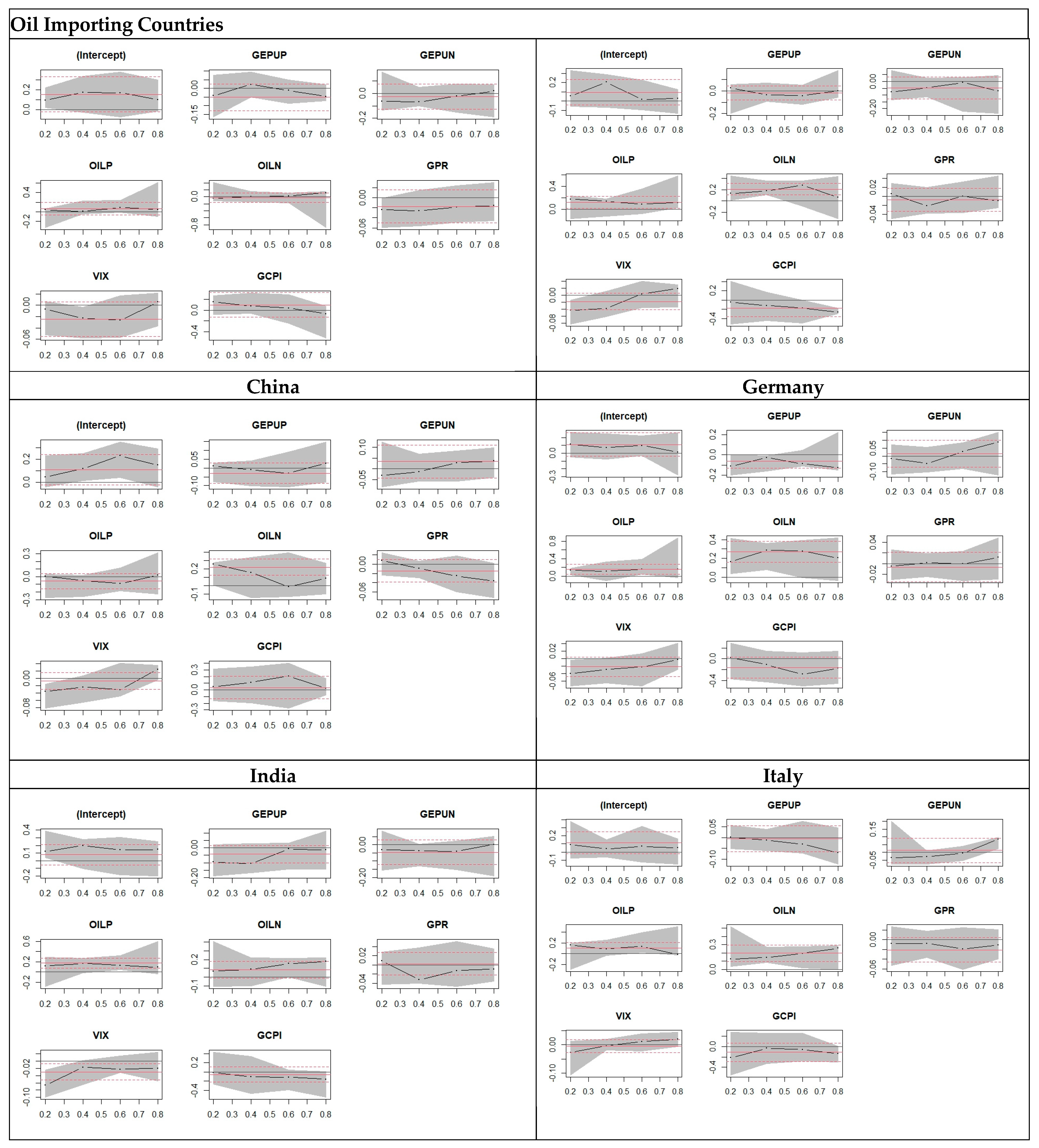
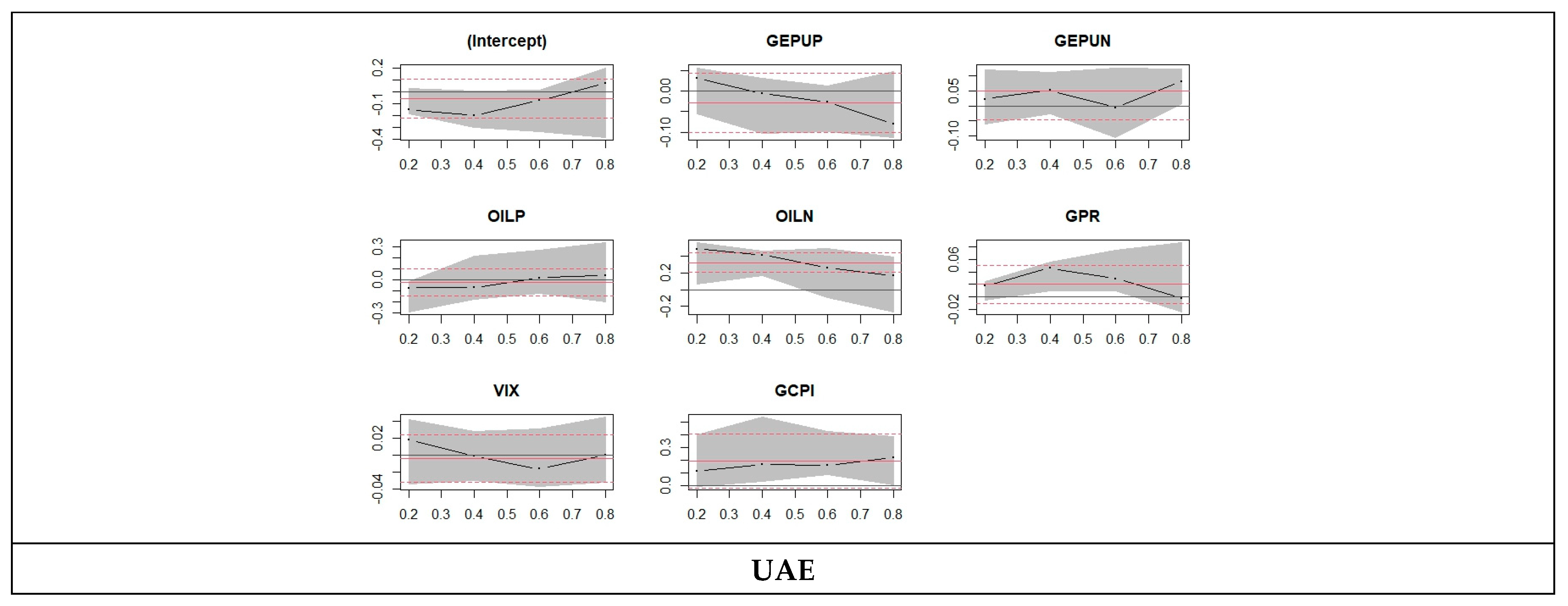
The results of oil-importing countries for asymmetric quantile regression are shown in Table 4. Where for the results of China, the GEPUp shocks show a decreasing trend, which shows that when GEPUp is at a high quantile, we can see lower market return, and when GEPUp is at a low quantile, we see higher market return. GEPUn shows an increasing trend, which indicates a higher market return at a high quantile and a lower market return at a low quantile. Coming to OILp (positive oil shocks), it shows a decreasing trend, which indicates a lower market return at high quantile and higher market return for lower quantile. Coming to OILn (negative oil shocks), an increasing trend is witnessed, which indicates a higher return at a higher quantile and a lower return at a lower quantile. In asymmetric quantile regression of Germany, the GEPUp shocks show a decreasing trend from 0.001 at the 0.2 quantile to −0.017 at the 0.8 quantile, which shows that when GEPUp is at a high quantile, we can see a low market return, and when GEPUp is at a low quantile, we see a high market return. GEPUn shows a decreasing trend. At the 0.2 quantile, GEPUn is −0.062, which shows that when GEPUn is at a lower quantile, we see a higher market return. At the 0.8 quantile, GEPUn is −0.072, which shows that when GEPUn is at a higher quantile, we see lower market return. Coming to OILp (positive oil shocks), it shows a constant trend moving from 0.079 at the 0.2 quantile to 0.079 at the 0.8 quantile, which indicates a lower return at a low quantile and higher market return for a higher quantile. Coming to OILn (negative oil shocks), an increasing trend from −0.025 at the 0.2 quantile to 0.152 at the 0.8 quantile is observed. This indicates a higher market return at a higher quantile and a lower market return at a lower quantile.
In asymmetric quantile regression of India, the GEPUp shocks show an increasing trend, which shows that when GEPUp is at a high quantile, we can see a higher market return, and when GEPUp is at a low quantile, we see a lower market return. GEPUn shows a decreasing trend, which indicates a lower market return at high quantile and a higher market return at low quantile. Coming to OILp (positive oil shocks), it shows an increasing trend, which indicates a higher market return at a high quantile and a lower market return for a lower quantile. Coming to OILn (negative oil shocks), a decreasing trend is witnessed, which indicates a lower return at a higher quantile and a higher return at a lower quantile.
In asymmetric quantile regression of Italy, the GEPUp shocks show an increasing trend from −0.095 at 0.2 quantile to −0.079 at 0.8 quantile, which shows that when GEPUp is at a high quantile, we can see higher market return, and when GEPUp is at a low quantile, we see lower market return. GEPUn shows an increasing trend. At the 0.2 quantile, GEPUn is −0.022, which shows that when GEPUn is at a lower quantile, we see lower market returns. At 0.8 quantile, GEPUn is 0.068, which shows that when GEPUn is at a higher quantile, we see a higher market return. Coming to OILp (positive oil shocks), it shows a decreasing trend moving from 0.075 at the 0.2 quantile to 0.051 at the 0.8 quantile, which indicates a higher return at the lower quantile and a lower market return for the higher quantile. Coming to OILn (negative oil shocks), an increasing trend from 0.116 at the 0.2 quantile to 0.289 at the 0.8 quantile is observed. This indicates a higher market return at a higher quantile and a lower market return at a lower quantile.
In asymmetric quantile regression of Japan, the GEPUp shocks show an increasing trend, which shows that when GEPUp is at a high quantile, we can see a higher market return, and when GEPUp is at a low quantile, we see a lower market return. GEPUn shows an increasing trend, which indicates a lower market return at low quantile and a higher market return at high quantile. Coming to OILp (positive oil shocks), it shows a decreasing trend, which indicates a higher market return at low quantiles and a lower market return for higher quantiles. Coming to OILn (negative oil shocks), an increasing trend is witnessed, which indicates a lower return at a lower quantile and a higher return at a higher quantile.
In asymmetric quantile regression of South Korea, the GEPUp shocks show an increasing trend, which shows that when GEPUp is at a high quantile, we can see higher market return, and when GEPUp is at a low quantile, we see lower market return. GEPUn shows an increasing trend, which indicates a lower market return at low quantile and a higher market return at high quantile. Contrary to these findings, in the asymmetric quantile regression of the USA, the GEPUp shocks show a decreasing trend, which shows that when GEPUp is at a high quantile, we can see lower market returns and when GEPUp is at a low quantile, we see higher market returns. GEPUn shows an increasing trend, which indicates a lower market return at low quantile and a higher market return at high quantile.
Figure 1 shows the asymmetric quantile regression of oil importing and exporting countries, and the horizental red lines are OLS regression cofficients that does not change accross quantile. Wheras the dashed lines sourrounding OLS regression line are the confidence interval. Whereas the black lines are quantile regression cofficients that changes over quantiles. From these figures we can compare the quantile cofficents at lower and upper quantile with ols regression cofficients.

4.3. Robustness Check: Standard Quantile Regression Model

The results in Table 5 show that at the 0.20 quantile of Canada, the GEPU value is 0.023, which is highly significant, and is greater than −0.010 at the 0.80 quantile, which is also highly significant. For Canada, we can see that according to stock market returns, the GEPU shows a decreasing effect from 0.20 quantile to 0.80, and we witness the same for oil as well. It shows a decreasing trend from 0.041 at the 0.20 quantile to 0.042 at the 0.80 quantile, both values being highly significant. At the 0.20 quantile of Iraq, the GEPU value is 0.093, which is highly significant and is greater than −0.018 at the 0.80 quantile, which is also highly significant. For Iraq, we can see that according to stock market returns, the GEPU shows a decreasing effect from 0.20 quantile to 0.80. Oil shows a decreasing trend from 0.040 at the 0.20 quantile to −0.008 at the 0.80 quantile. Both of the values are insignificant, showing that it has no real effect. At 0.20 quantile of Russia, the GEPU value is 0.099, which is highly significant and is less than 0.028 at the 0.80 quantile, which is insignificant, showing no effect. For Russia, we can see that according to stock market returns, the GEPU shows a decreasing effect from 0.20 quantile to 0.80. Oil shows an increasing trend from 0.013 at the 0.20 quantile to 0.616 at the 0.80 quantile. Both of the values are highly significant, showing that it has an effect.
At the 0.20 quantile of Saudia, the GEPU value is 0.019, which is insignificant and is less than 0.054 at the 0.80 quantile, which is significant, showing no effect. For Saudia, we can see that according to stock market returns, the GEPU shows an increasing effect from 0.20 quantile to 0.80. Oil shows an increasing trend from 0.025 at the 0.20 quantile to 0.295 at the 0.80 quantile. Both of the values are highly significant, showing that it has an effect. At the 0.20 quantile of UAE, the GEPU value is 0.051, which is more than −0.068 at the 0.80 quantile, both being insignificant and showing no effect. For the UAE, we can see that according to stock market returns, the GEPU shows a decreasing effect from the 0.20 quantile to the 0.80. Oil shows an increasing trend from −0.148 at the 0.20 quantile to 0.016 at the 0.80 quantile. Both of the values are insignificant, showing that it has no effect.
The results in Table 6 Show that at the 0.20 quantile of China, the GEPU value is −0.009, which is less than −0.062 at the 0.80 quantile; the value is insignificant at the 0.20 quantile, and it is significant at the 0.80 quantile. For China, we can see that according to stock market returns, the GEPU shows an increasing effect from 0.20 quantile to 0.80, and we witness the same for oil as well. It shows an increasing trend from −0.010 at the 0.20 quantile to 0.015 at the 0.80 quantile, both values are insignificant, showing no true effect. At the 0.20 quantile of Germany, the GEPU value is 0.035, which is significant, which is greater than −0.009 at the 0.80 quantile, which is insignificant. For Germany, we can see that according to stock market returns, the GEPU shows a decreasing effect from 0.20 quantile to 0.80. Oil shows a decreasing trend from 0.035 being insignificant at the 0.20 quantile to 0.031 at the 0.80 quantile, being significant and showing a true effect. At the 0.20 quantile of India, the GEPU value is 0.008, which is less than 0.025 at the 0.80 quantile, both of which are insignificant values. For India, we can see that according to stock market returns, the GEPU shows an increasing effect from 0.20 quantile to 0.80. Oil shows a decreasing trend from 0.039 at the 0.20 quantile to 0.017 at the 0.80 quantile, showing a significant effect at the 0.20 quantile while having no significant effect at the 0.80 quantile.
At the 0.20 quantile of Italy, the GEPU value is 0.015, which is greater than −0.004 at the 0.80 quantile; both of these values are insignificant. For Italy, we can see that according to stock market returns, the GEPU shows a decreasing effect from 0.20 quantile to 0.80. Oil shows a decreasing trend from 0.018 at the 0.20 quantile to 0.023 at the 0.80 quantile; both values are insignificant. At the 0.20 quantile of Japan, the GEPU value is −0.016, which is less than −0.012 at the 0.80 quantile; both values are insignificant. For Japan, we can see that according to stock market returns, the GEPU shows a decreasing effect from 0.20 quantile to 0.80. Oil shows a decreasing trend from 0.015 at the 0.20 quantile to 0.008 at the 0.80 quantile, both values are insignificant.
Likewise, 
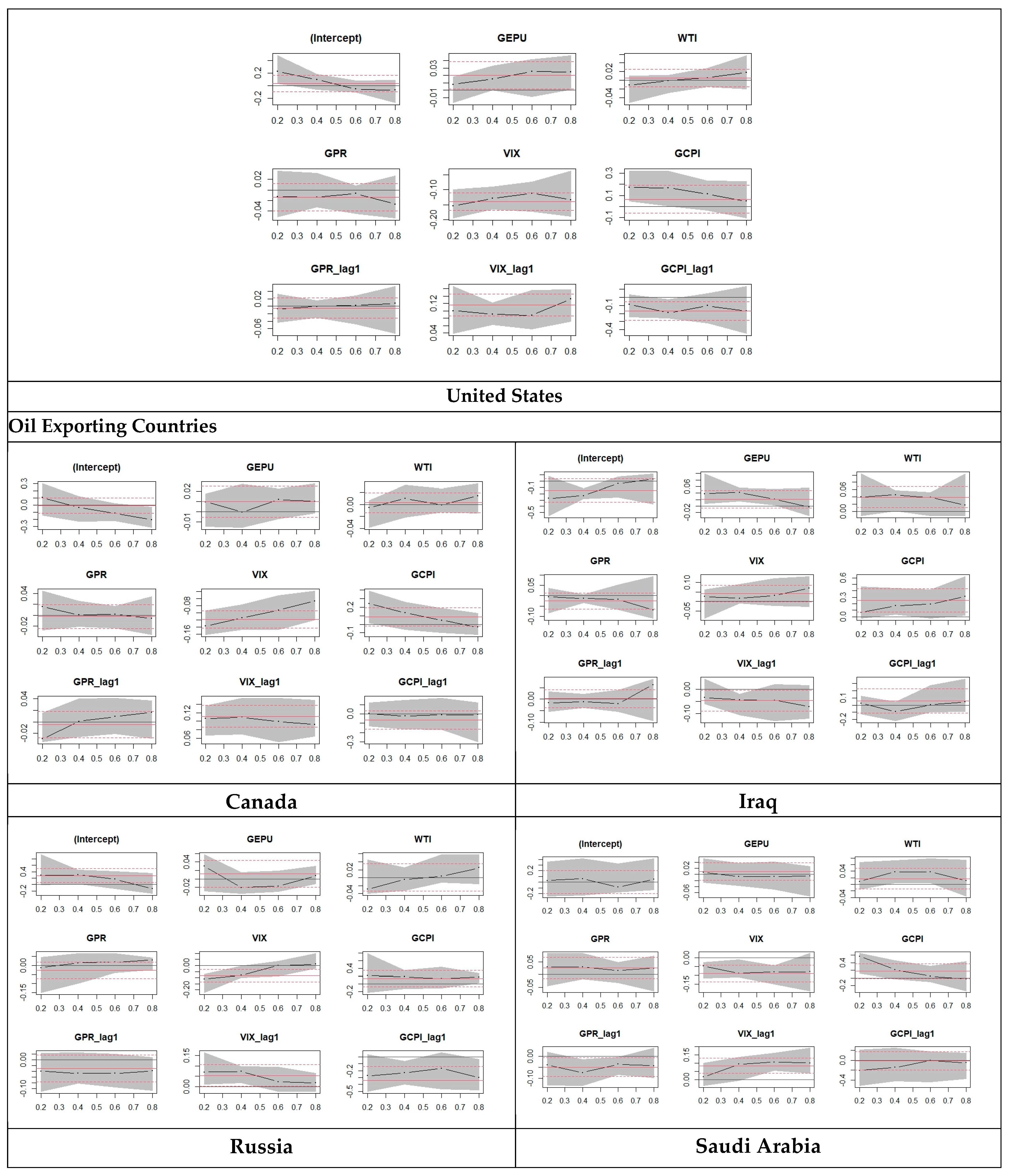
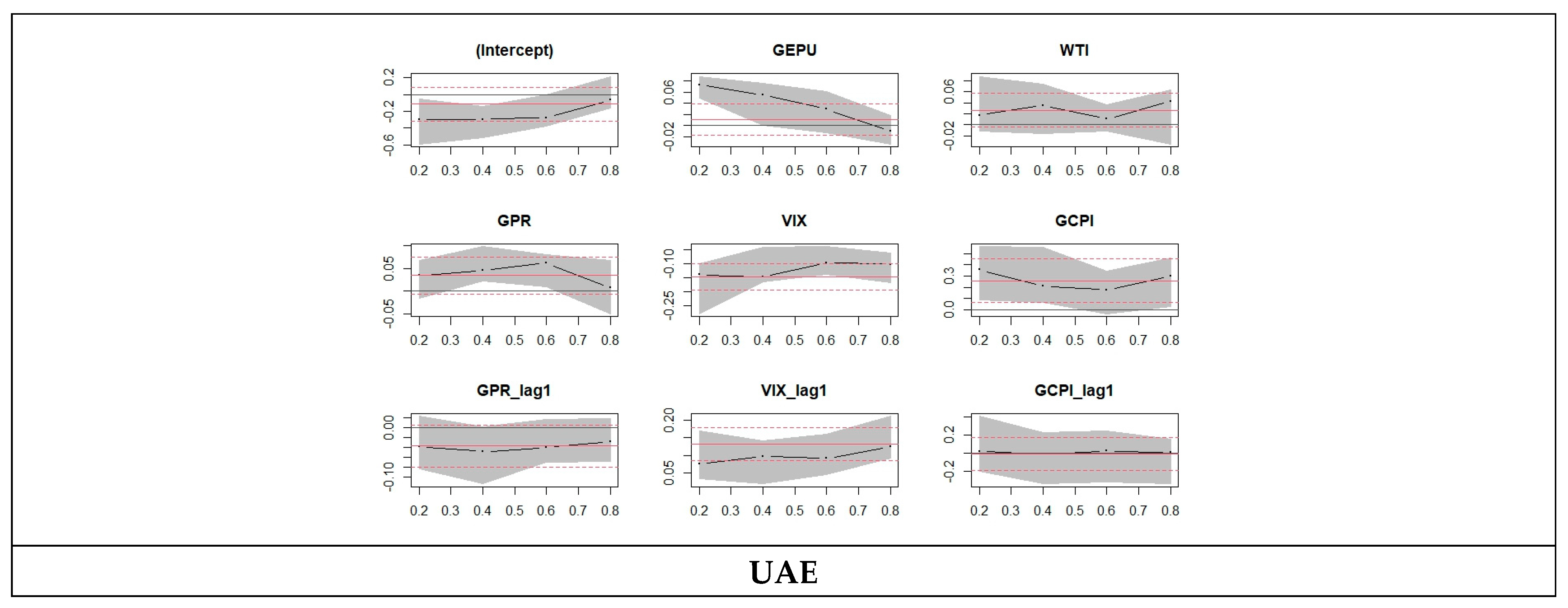
Table 7 depicts the quintile regression of oil exporting countries at lower and higher quintile regression, and there are mixture of trends, increasing as well as decreasing shown in various countries.
Figure 2 depicts the findings of quantile regression of oil exporting and importing countris in pictorial form, and the horizental red lines are OLS regression cofficients that does not change accross quantile. Wheras the dashed lines sourrounding OLS regression line are the confidence interval. Whereas the black lines are quantile regression cofficients that changes over quantiles. From these figures we can compare the quantile cofficents at lower and upper quantile with ols regression cofficients.

5. Conclusions

We employ quantile regression (QR) analysis to study the asymmetric effects of changes in oil price and EPU on the stock market returns of the major oil importing and exporting countries. QR analysis provides information on the co-movement between stock returns and changes in oil price and EPU. We allow for asymmetries by differentiating between positive and negative changes in oil prices and EPU. We used monthly data from May 2014 to December 2024 and estimated four models for each country: symmetric and asymmetric OLS and QR models.
The symmetric OLS model for oil-exporting countries shows that while changes in EPU hurt the stock returns in all countries except Iraq, where it shows a positive but insignificant effect, oil price changes have a positive effect in all countries, whereas for oil-exporting countries they show that while changes in EPU have an inverse impact on the stock market returns in all countries, moreover, for oil price changes they have a positive effect on the stock returns in all countries and a negative but insignificant effect in Iraq and the UAE. In contrast, the asymmetric OLS model shows that while positive changes in EPU have an inverse effect on the stock returns in all the countries, negative changes are insignificant in all the countries, and these findings align with the results of the study conducted by Managi et al. (2022) during the COVID-19 pandemic.
This indicates that positive and negative changes in EPU have asymmetric effects on stock returns since rising EPU lowers stock returns, whereas falling EPU is insignificant. We find that positive oil price changes have an insignificant effect for both oil-importing and oil-exporting countries, except Canada and Russia, where they show a significant effect. Moreover, we find that negative oil price changes have a significant effect on all major oil-importing and -exporting countries except for Iraq, Russia, and China. Similarly, the symmetric QR model for oil-importing countries shows that while EPU harms the stock returns of all the countries except for Iraq, across the entire quantile distribution, the stock returns and oil price changes have a positive significant effect on the stock returns in all countries and an insignificant effect in Iraq. Whereas for oil-exporting countries, it shows that while EPU has a negative effect on the stock returns of all the countries across the entire quantile distribution on the stock returns and for oil price changes, it also shows a positive significant effect on the stock returns in all oil-importing countries.
On the other hand, for oil-exporting countries, the asymmetric QR models show that while positive changes in EPU have a negative effect on stock returns in Canada, Russia, Saudi Arabia, and UAE across all of the quantiles, except for Iraq, where it shows a positive effect. Negative changes are significant, while positive changes in Iraq are insignificant. This shows that changes in EPU have an asymmetric effect on the stock market returns since rising EPU reduces stock market returns, however, decreasing EPU is insignificant in most of the quantile for all the countries, except it shows low and medium significance in the medium quantile of Iraq, Russia, and UAE. As for oil, it shows that while positive changes in oil prices show a positive effect in all countries except for Iraq, negative changes show a positive but insignificant effect in all oil-exporting countries. We find the decreasing oil prices reduce the stock market returns in all countries during almost all quantiles.
In contrast to that, for oil-importing countries, the asymmetric QR models show that positive changes in EPU have a negative effect on stock returns in all countries across all of the quantiles, where changes are significant. This shows that changes in EPU have an asymmetric effect on the stock market returns since rising EPU reduces stock market returns; however, decreasing EPU is insignificant in all of the quantiles for all the countries. As for oil, it shows that while positive changes in oil prices show a positive effect in all countries with insignificant values in low and medium quantiles while significant values in the high qauntile moreover, we can see that some negative effects in the high quantile for China. The negative changes show a positive effect in all oil-importing countries, except China, whereas all positive effects are significant and negative effects are insignificant.

6. Implications

Our research findings have some important policy implications. First, because the impacts of changes in oil price and EPU are not the same and changes throughout the distribution of the stock returns, policy recommendations can be drawn based on the results of OLS since it can be misleading. Second, our results show that changes in oil price and EPU have massive effects on the stock returns of oil-importing and oil-exporting countries, which seem to be asymmetric and change according to the conditions of the market. Thus, policymakers should pay close attention to variations in oil price and EPU. They should be able to know how to respond to these changes in order to avoid adverse consequences. For instance, EPU shows a decreasing trend for Italy and India, which means that the stock market return is affected and decreases when there are fluctuations in the EPU, so investors are required to give full attention to such countries, whereas countries such as Canada and the USA show an increasing trend, which gives insights to investors and policymakers not to respond to falling EPU. Also, our results show that the influence of positive changes in EPU is more significant and larger than that of the negative changes. This indicates that policymakers and investors should devote more attention to rising EPU than to falling EPU.
Lastly, positive changes in oil prices appear to carry more significance in most countries compared to negative changes. The resulting impact is generally positive, especially in the midst of extreme market conditions. As a consequence, policymakers are encouraged to allocate greater attention to the ascent of oil prices rather than their decline. It is advisable for policymakers to steer clear of uncertain information related to oil price shifts, as such ambiguity has the potential to induce heightened volatility in stock markets. A balanced approach to addressing both positive and negative changes in oil prices is crucial for comprehensive economic management. In addition, they may need to coordinate efforts internationally to manage the effects of oil price fluctuations on a global scale. To conclude, investors and policymakers need to come up with a holistic approach that takes into account both short-term responses to extreme market conditions and long-term strategies for managing oil price fluctuations.

7. Limitations and Future Recommendations

This research has its own limitations, as it is only restricted to the context of selected oil-importing and exporting countries. Future researchers can opt for conducting the same study for other oil-importing countries such as the UK, France, Spain, and Nigeria, and oil-exporting countries such as Malaysia, Norway, Brazil, and Kuwait that are not selected in this research for comparative analysis. Another limitation of the study is that the insufficient data of 2023 makes it difficult for us to interpret the conclusion for the 2023 time period. In addition, as this study only focuses on macroeconomic factors such as market returns, oil prices, oil returns, and economic policy uncertainty, future researchers may add more factors such as unemployment rates and political risk to generalize the findings.

Author Contributions

Conceptualization, S.A. and H.Z.; methodology, A.B.; software, M.H.N.; validation, E.T. and A.B.; formal analysis, H.Z.; investigation, S.A.; resources, A.B.; data curation, E.T.; writing—original draft preparation, A.B.; writing—review and editing, H.Z.; visualization, E.T.; supervision, M.H.N.; project administration, S.A.; funding acquisition, A.B. All authors have read and agreed to the published version of the manuscript.

Funding

This research received no external funding.

Data Availability Statement

The original contributions presented in this study are included in the article. Further inquiries can be directed to the corresponding author(s).

Acknowledgments

We thank the editors of the journal for their guidance.

Conflicts of Interest

The authors declare no conflict of interest.

References

  1. Alamgir, Farzana, and Sakib Bin Amin. 2021. The nexus between oil price and stock market: Evidence from South Asia. Energy Reports 7: 693–703. [Google Scholar] [CrossRef]
  2. Aloui, Riadh, Rangan Gupta, and Stephen M. Miller. 2016. Uncertainty and crude oil returns. Energy Economics 55: 92–100. [Google Scholar] [CrossRef]
  3. Al-Thaqeb, Saud Asaad, Barrak Ghanim Algharabali, and Khaled Tareq Alabdulghafour. 2022. The pandemic and economic policy uncertainty. International Journal of Finance & Economics 27: 2784–94. [Google Scholar] [CrossRef]
  4. Antonakakis, N., I. Chatziantoniou, and G. Filis. 2014. Dynamic spillovers between oil and stock markets in the Gulf Cooperation Council Countries. Energy Economics 36: 28–42. [Google Scholar]
  5. Arbatli, Elif C., Steven J. Davis, Arata Ito, and Naoko Miake. 2019. Policy Uncertainty in Japan (August 5, 2019). Becker Friedman Institute for Research in Economics Working Paper No. 2017-09. Available online: https://ssrn.com/abstract=2972891 (accessed on 23 March 2022).
  6. Arouri, Mohamed, Christophe Estay, Christophe Rault, and David Roubaud. 2016. Economic policy uncertainty and stock markets: Longrun evidence from the US. Finance Research Letters 18: 136–41. [Google Scholar]
  7. Backus, David K., and Mario J. Crucini. 2000. Oil prices and the terms of trade. Journal of International Economics 50: 185–213. [Google Scholar]
  8. Bahmani-Oskooee, Mohsen, and Sujata Saha. 2019a. On the effects of policy uncertainty on stock prices. Journal of Economics and Finance 43: 764–78. [Google Scholar]
  9. Bahmani-Oskooee, Mohsen, and Sujata Saha. 2019b. On the effect of policy uncertainty on stock prices: An asym- metric analysis. Quantitative Finance and Economics 3: 412–24. [Google Scholar] [CrossRef]
  10. Baker, Scott R., Nicholas Bloom, and Steven J. 2016. Measuring economic policy uncertainty. The Quarterly Journal of Economics 131: 1593–636. [Google Scholar] [CrossRef]
  11. Basher, Syed A., and Perry Sadorsky. 2006. Oil price risk and emerging stock markets. Global Finance Journal 17: 224–51. [Google Scholar]
  12. Batabyal, Sourav, and Robert Killins. 2021. Economic policy uncertainty and stock market returns: Evidence from Canada. The Journal of Economic Asymmetries 24: e00215. [Google Scholar] [CrossRef]
  13. Chiang, Thomas C. 2019. Economic Policy Uncertainty, Risk and Stock Returns: Evidence from G7 Stock Markets. Finance Research Letters 29: 41–49. [Google Scholar] [CrossRef]
  14. Christou, Christina, Juncal Cunado, Rangan Gupta, and Christis Hassapis. 2017. Economic Policy Uncertainty and Stock Market Returns in PacificRim Countries: Evidence Based on a Bayesian Panel VAR Model. Journal of Multinational Financial Management 40: 92–102. [Google Scholar] [CrossRef]
  15. Civcir, Irfan, and Ugur Akkoc. 2021. Non-linear ARDL approach to the oil-stock nexus: Detailed sectoral analysis of the Turkish stock market. Resources Policy 74: 102424. [Google Scholar] [CrossRef]
  16. Cologni, Alessandro, and Matteo Manera. 2008. Oil price, infation and interest rates in a structural cointegrated VAR model for the G-7 countries. Energy Economics 30: 856–88. [Google Scholar]
  17. Cunado, Juncal, and Fernando Perez de Gracia. 2014. Oil price shocks and stock market returns: Evidence for some European countries. Energy Economics 42: 365–77. [Google Scholar] [CrossRef]
  18. Das, Debojyoti, and M. Kannadhasan. 2020. The asymmetric oil price and policy uncertainty shock exposure of emerging market sectoral equity returns: A quantile regression approach. International Review of Economics & Finance 9: 563–81. [Google Scholar]
  19. Degiannakis, Stavros, George Filis, and Vipin Arora. 2018. Oil prices and stock markets: A review of the theory and empirical evidence. The Energy Journal 39: 85–130. [Google Scholar]
  20. Diaz, Elena Maria, Juan Carlos Molero, and Fernando Perez De Gracia. 2016. Oil price volatility and stock returns in the G7 economies. Energy Economics 54: 417–30. [Google Scholar]
  21. Hamilton, James D. 1983. Oil and the macro economy since World War II. Journal of Political Economy 91: 228–48. [Google Scholar]
  22. Hamilton, James D. 1996. This is what happened to the oil price-macroeconomy relationship. Journal of Monetary Economics 38: 215–20. [Google Scholar]
  23. Hamilton, James D. 2009. Causes and Consequences of the Oil Shock of 2007-08 (No. w15002). Cambridge, MA: National Bureau of Economic Research, pp. 215–61. Available online: https://www.nber.org/papers/w15002 (accessed on 23 March 2022).
  24. Henriques, Irene, and Perry Sadorsky. 2008. Oil prices and the stock prices of alternative energy companies. Energy Economics 30: 998–1010. [Google Scholar]
  25. Herrera, Ana María, Latika Gupta Lagalo, and Tatsuma Wada. 2015. Asymmetries in the Response of Economic Activity to Oil Price Increases and Decreases? Journal of International Money and Finance 50: 108–33. [Google Scholar]
  26. Jeris, Saeed Sazzad, and Ridoy Deb Nath. 2020. COVID-19, oil price and UK economic policy uncertainty: Evidence from the ARDL approach. Quantitative Finance and Economics 4: 503–14. [Google Scholar]
  27. Kang, Wensheng, and Ronald A. Ratti. 2013. Oil shocks, policy uncertainty, and stock market returns. Journal of International Financial Markets, Institutions and Money 26: 305–18. [Google Scholar]
  28. Kilian, Lutz. 2009. Not all oil price shocks are alike: Disentangling demand and supply shocks in the crude oil market. American Economic Review 99: 1053–69. [Google Scholar]
  29. Kilian, Lutz, and Cheolbeom Park. 2009. The impact of oil price shocks on the US stock market. International Economic Review 50: 1267–87. [Google Scholar]
  30. Koenker, Roger, and Gilbert Bassett. 1978. Regression quantiles. Econometrica 46: 33–50. [Google Scholar]
  31. Laakkonen, Helinä, and Markku Lanne. 2008. Asymmetric News Efects on Volatility: Good vs. Bad News in Good vs. Bad Times. Discussion Paper No. 207. Helsinki: Helsinki Center of Economic Research. ISSN 1795–0562. [Google Scholar]
  32. Lee, Kiseok, Shawn Ni, and Ronald A. Ratti. 1995. Oil shocks and the macroeconomy: The role of price variability. The Energy Journal 16: 39–56. [Google Scholar]
  33. Lin, Boqiang, and Rui Bai. 2021. Oil prices and economic policy uncertainty: Evidence from global, oil importers, and exporters’ perspective. Research in International Business and Finance 56: 101–357. [Google Scholar]
  34. Managi, Shunsuke, Mohamed Yousfi, Younes Ben Zaied, Nejah Ben Mabrouk, and Béchir Ben Lahouel. 2022. Oil price, US stock market and the US business conditions in the era of COVID-19 pandemic outbreak. Economic Analysis and Policy 73: 129–39. [Google Scholar] [PubMed]
  35. Mensi, Walid, Shawkat Hammoudeh, Juan Carlos Reboredo, and Duc Khuong Nguyen. 2014. Do global factors impact BRICS stock markets? A quantile regression approach. Emerging Markets Review 19: 1–17. [Google Scholar] [CrossRef]
  36. Mork, Knut Anton. 1989. Oil and the macroeconomy when prices go up and down: An extension of Hamilton’s results. Journal of Political Economy 97: 740–44. [Google Scholar]
  37. Naifar, Nader. 2015. Do global risk factors and macroeconomic conditions affect global Islamic index dynamics? A quantile regression approach. The Quarterly Review of Economics and Finance 61: 29–39. [Google Scholar]
  38. Nazir, Sidra, and Abdul Qayyum. 2014. Impact of Oil Price and Shocks on Economic Growth of Pakistan: Multivariate Analysis. Munich: Munich Personal RePEc Archive. [Google Scholar]
  39. Nusair, Salah A., and Dennis Olson. 2019. The effects of oil price shocks on Asian exchange rates: Evidence from quantile regression analysis. Energy Economics 78: 44–63. [Google Scholar]
  40. Nusair, Salah A., and Jamal A. Al-Khasawneh. 2018. Oil price shocks and stock market returns of the GCC countries: Empirical evidence from quantile regression analysis. Economic Change and Restructuring 51: 339–72. [Google Scholar]
  41. Nusair, Salah A., and Jamal A. Al-Khasawneh. 2022. Impact of economic policy uncertainty on the stock markets of the G7 Countries: A nonlinear ARDL approach. The Journal of Economic Asymmetries 26: e00251. [Google Scholar]
  42. Qin, Meng, Chi-Wei Su, Lin-Na Hao, and Ran Tao. 2020. The stability of US economic policy: Does it really matter for oil price? Energy 198: 117315. [Google Scholar]
  43. Rehman, Mobeen Ur. 2018. Do oil shocks predict economic policy uncertainty? Physica A: Statistical Mechanics and Its Applications 498: 123–36. [Google Scholar]
  44. Sadorsky, Perry. 1999. Oil price shocks and stock market activity. Energy Economics 21: 449–69. [Google Scholar]
  45. Soroka, Stuart N. 2006. Good news and bad news: Asymmetric responses to economic information. The Journal of Politics 68: 372–85. [Google Scholar]
  46. Synergen. 2020. Top 6 Events That Impacted Global Oil Prices. SynergenOG. Available online: https://synergenog.com/top-6-events-that-impacted-global-oil-prices/ (accessed on 23 March 2022).
  47. Wang, Yudong, Chongfeng Wu, and Li Yang. 2013. Oil price shocks and stock market activities: Evidence from oil-importing and oil-exporting countries. Journal of Comparative Economics 41: 1220–39. [Google Scholar]
  48. You, Wanhai, Yawei Guo, Huiming Zhu, and Yong Tang. 2017. Oil price shocks, economic policy uncertainty and industry stock returns in China: Asymmetric efects with quantile regression. Energy Economics 68: 1–18. [Google Scholar]
  49. Zhou, John. 2015. The Good, the Bad, and the Ambiguous: The Aggregate Stock Market Dynamics Around mac-Roeconomic News. Available online: https://papers.ssrn.com/sol3/papers.cfm?abstract_id=2555050 (accessed on 24 January 2015).
  50. Zhu, Huiming, Yawei Guo, Wanhai You, and Yaqin Xu. 2016. The heterogeneity dependence between crude oil price changes and industry stock market returns in China: Evidence from quantile regression approach. Energy Economics 55: 30–41. [Google Scholar]
Figure 1. Plot for asymmetric quantile regression.
Risks 13 00093 g001aRisks 13 00093 g001bRisks 13 00093 g001c
Figure 2. Plot for quantile regression.
Risks 13 00093 g002aRisks 13 00093 g002bRisks 13 00093 g002c
Table 1. Description of variables.
VariablesSymbolsMeasurementMeasurement
Oil Importing CountriesChina, Germany, India, Italy, Japan, South Korea, United States
Oil Exporting CountriesCanada, Iraq, Russia, Saudi Arabia, UAE
Data FrameMonthly data from May 2014 to Dec 2024
Dependent Variable
Logarithmic returns of major index prices of each importing and exporting countryRiln(Current period value/previous period value)Investing.com
Independent Variables
Global Economic Policy UncertaintyGEPUln(GEPU)Policy uncertainty.com
Crude Oil WTIWTIln(WTI)Investing.com
Control Variables
Global Geopolitical Risk IndexGPRln(GPR)Policy uncertainty.com
CBOE Volatility IndexVIXln(VIX)Investing.com
Global Price Index of All CommoditiesGCPIln(Current period value/previous period value)fred.stlouisfed.org
We have included three control variables to address omitted variable bias and their lagged terms as instrumental variables to address the possibility of endogeneity issues. Therefore, our model is now an instrumental variable quantile regression model with the asymmetric effect of global economic policy uncertainty (GEPU) and crude oil WTI (WTI). These three variables include the Global Geopolitical Risk Index (GPR), the CBOE Volatility Index (VIX), and the Global Price Index of All Commodities (GCPI). We included these three control variables because of their global impact on returns, which are not related to returns of a specific market but impact all markets globally.
Table 2. Descriptive statistics.
MeanStdMaxMinSkewnessKurtosisJBADF
CHINA0.00390.05830.1871−0.2568−0.20376.619570.2048 ***−9.6160 ***
GERMANY0.00550.04940.1399−0.1796−0.36514.00898.2077 **−11.6052 ***
INDIA0.00930.04690.1370−0.2646−1.374010.9448373.9653 ***−11.7018 ***
ITALY0.00670.05650.2075−0.2540−0.58746.692079.4342 ***−12.1937 ***
JAPAN0.00790.04660.1401−0.1112−0.46753.28495.0557 *−11.4191 ***
SK0.00150.04750.1337−0.1436−0.48494.395315.2785 ***−12.2577 ***
US0.00740.04350.1306−0.1478−0.33804.11098.9485 **−12.6762 ***
CANADA0.00410.03720.0997−0.1952−1.15278.8138206.9849 ***−12.6196 ***
IRAQ0.00050.05160.1394−0.13460.14413.56772.1448−10.2206 ***
RUSSIA0.00550.06240.1653−0.3570−1.805211.5956459.9428 ***−12.1135 ***
SA0.00160.05680.1521−0.1902−0.54273.870110.2401 ***−10.7098 ***
UAE0.00010.06680.2036−0.3799−1.554312.0476484.3104 ***−13.6840 ***
GEPU5.31700.35176.06794.4621−0.36832.45784.4268−3.2681 **
GEPUP0.07140.12280.62810.00002.546510.1314406.3795 ***−13.6092 ***
GEPUN−0.06130.09320.0000−0.5000−1.83256.4980135.8266 ***−13.2468 ***
WTI4.10340.31054.74212.9360−0.64254.254617.0659 ***−2.7112 *
OILP0.04150.07310.63330.00004.678135.57456078.1981 ***−10.4512 ***
OILN−0.04430.08800.0000−0.7819−5.110040.49437991.8453 ***−9.1578 ***
GPR4.63830.27055.76504.06770.72794.554924.0071 ***−4.6778 ***
VIX2.84000.31054.05592.31510.75163.877916.0344 ***−3.8529 ***
GCPI−0.00010.04770.1644−0.1673−0.33124.629316.3681 ***−7.6459 ***
JB is the Jarque–Bera test for normality. Std is the standard deviation, and ADF is the Augmented Dickey-Fuller test for checking stationarity. *, **, *** indicates significance at 10%, 5%, and 1% respectively.
Table 3. Correlation matrix.
GEPUGEPUPGEPUNWTIOILPOILNGPRVIXGCPI
GEPU1
GEPUP0.26141
GEPUN0.14470.38521
WTI−0.0133−0.11500.02411
OILP0.1670−0.0248−0.0436−0.07531
OILN−0.0537−0.2357−0.19480.33360.28871
GPR−0.03670.07730.02280.4584−0.20180.02491
VIX0.52230.19100.0810−0.17920.1210−0.3345−0.07961
GCPI0.0921−0.0871−0.21740.16130.36720.5745−0.0559−0.13611
Table 4. Asymmetric quantile regression (oil importing countries).
q = 0.20q = 0.40q = 0.60q = 0.80
CountryVariablesCoefficientsSigCoefficientsSigCoefficientsSigCoefficientsSig
CHINA(Intercept)0.1130.1760.1900.0830.2380.030−0.0310.875
GEPUP0.0010.9810.0560.2080.0220.616−0.0220.784
GEPUN−0.0370.405−0.0570.326−0.0400.4880.0460.659
OILP−0.0540.351−0.0550.4670.0390.6090.0910.504
OILN−0.1700.006−0.0490.532−0.0360.646−0.1320.346
GPR−0.0410.035−0.0300.232−0.0030.908−0.0110.813
VIX−0.1300.000−0.0870.006−0.0880.005−0.1530.007
GCPI0.1840.0930.0780.5870.0680.6330.0410.873
GPR_lag10.0110.592−0.0020.937−0.0330.2100.0220.630
VIX_lag10.1260.0000.0670.0250.0640.0320.1590.003
GCPI_lag1−0.0970.258−0.1460.191−0.1710.1260.0840.671
GERMANY(Intercept)0.2130.0490.0110.9010.0270.838−0.0020.983
GEPUP0.0010.9830.0120.742−0.0160.767−0.0170.716
GEPUN−0.0620.277−0.0420.368−0.0420.553−0.0720.226
OILP0.0790.292−0.0100.876−0.0030.9700.0790.312
OILN−0.0250.7430.0680.2830.0820.3890.1520.062
GPR−0.0250.3260.0090.6620.0160.6000.0370.153
VIX−0.1740.000−0.1390.000−0.1410.000−0.1380.000
GCPI−0.0640.646−0.0070.952−0.0730.671−0.2460.094
GPR_lag1−0.0170.515−0.0180.403−0.0190.555−0.0320.231
VIX_lag10.1540.0000.1490.0000.1420.0000.1440.000
GCPI_lag1−0.0320.771−0.1790.048−0.1480.275−0.1820.114
INDIA(Intercept)0.1400.2050.1430.2570.1220.3220.2420.069
GEPUP−0.0680.1310.0020.974−0.0010.9800.0640.237
GEPUN0.0110.857−0.0160.8090.0350.5890.0680.330
OILP−0.0480.534−0.1090.217−0.1380.109−0.0080.932
OILN0.1470.0650.2200.0170.1570.0790.1740.070
GPR0.0060.8230.0060.8450.0050.862−0.0090.773
VIX−0.0910.004−0.0940.010−0.0970.006−0.1160.003
GCPI−0.0300.834−0.0780.6370.0020.990−0.0490.778
GPR_lag1−0.0270.300−0.0280.349−0.0230.437−0.0440.169
VIX_lag10.0740.0140.0840.0150.0960.0050.1350.000
GCPI_lag10.0900.425−0.0610.633−0.0120.923−0.0290.832
ITALY(Intercept)0.2130.0380.0990.3810.1070.2030.0970.436
GEPUP−0.0950.023−0.0310.500−0.0290.394−0.0790.123
GEPUN−0.0220.690−0.0370.5380.0640.1510.0680.308
OILP0.0750.2920.0230.7700.1180.0450.0510.556
OILN0.1160.1150.1990.0170.1860.0030.2980.001
GPR−0.0060.8150.0120.6480.0230.245−0.0040.903
VIX−0.1300.000−0.1120.001−0.1380.000−0.0840.019
GCPI−0.1610.230−0.1300.382−0.0730.505−0.0980.549
GPR_lag1−0.0320.187−0.0240.384−0.0260.193−0.0180.543
VIX_lag10.1100.0000.0970.0020.1160.0000.1080.002
GCPI_lag1−0.0400.698−0.1180.310−0.1930.025−0.1950.128
JAPAN(Intercept)0.0970.1660.1190.1880.2090.016−0.0200.767
GEPUP−0.0690.016−0.0740.044−0.0400.2480.0250.375
GEPUN−0.0380.300−0.0160.733−0.0100.8230.0050.892
OILP0.1190.0150.0860.1730.0800.1830.0700.146
OILN0.0020.975−0.0240.7150.0760.2180.0570.252
GPR0.0340.0350.0050.817−0.0230.251−0.0030.834
VIX−0.1920.000−0.1140.000−0.0960.000−0.1130.000
GCPI−0.1900.039−0.0610.602−0.1370.222−0.0460.610
GPR_lag1−0.0380.025−0.0240.263−0.0180.3850.0190.255
VIX_lag10.1550.0000.1030.0000.0960.0000.1080.000
GCPI_lag1−0.0630.373−0.1510.103−0.2100.018−0.0490.486
SOUTH KOREA(Intercept)0.2120.1020.0630.512−0.0450.5120.0140.897
GEPUP0.0050.931−0.0190.6330.0060.8390.0140.751
GEPUN−0.0450.512−0.0060.9120.0150.6710.0590.300
OILP0.0380.6710.0850.2100.1120.0190.1940.010
OILN0.1440.1240.1410.0440.1510.0020.0890.247
GPR−0.0130.665−0.0060.782−0.0020.902−0.0260.297
VIX−0.0970.010−0.0630.024−0.0540.006−0.1060.001
GCPI−0.1820.282−0.1330.295−0.0750.397−0.0830.552
GPR_lag1−0.0290.356−0.0120.611−0.0080.6380.0200.445
VIX_lag10.0810.0220.0690.0090.0900.0000.1240.000
GCPI_lag1−0.2530.057−0.1490.133−0.1810.010−0.0480.663
UNITED STATES(Intercept)0.2120.0180.1800.0080.0690.2570.0890.329
GEPUP0.0820.0250.0500.0660.0690.0060.0410.266
GEPUN−0.0440.349−0.0030.932−0.0050.8780.0710.148
OILP0.0380.540−0.0070.8770.1360.0020.0240.709
OILN0.0250.6960.1240.0120.1070.0160.2010.003
GPR0.0000.9930.0040.8210.0030.860−0.0070.736
VIX−0.1480.000−0.1320.000−0.1180.000−0.0840.002
GCPI0.1820.1190.0330.708−0.0470.557−0.1370.254
GPR_lag1−0.0210.325−0.0240.135−0.0140.336−0.0090.693
VIX_lag10.0990.0000.1020.0000.1160.0000.0940.000
GCPI_lag1−0.0770.395−0.1450.036−0.1580.012−0.1260.180
Table 5. Asymmetric quantile regression (oil exporting countries).
q = 0.20q = 0.40q = 0.60q = 0.80
CountryVariablesCoefficientsSigCoefficientsSigCoefficientsSigCoefficientsSig
CANADA(Intercept)0.0750.120−0.0090.843−0.0500.484−0.1020.195
GEPUP0.0230.2360.0320.0870.0080.793−0.0100.762
GEPUN−0.0070.7830.0160.5030.0410.2780.0400.337
OILP0.0410.2190.0570.079−0.0220.6550.0420.441
OILN0.1150.0010.1120.0010.1670.0020.1220.034
GPR0.0040.7060.0130.2420.0110.5230.0140.455
VIX−0.0840.000−0.1130.000−0.1040.000−0.0650.004
GCPI0.0360.563−0.0200.744−0.1400.135−0.1010.330
GPR_lag1−0.0150.210−0.0100.357−0.0040.834−0.0030.891
VIX_lag10.0690.0000.1120.0000.1180.0000.0940.000
GCPI_lag10.0960.0540.0480.3130.0250.7280.0160.843
IRAQ(Intercept)−0.1700.2170.0330.7860.0660.5110.0920.620
GEPUP0.0930.0980.0560.2670.0440.282−0.0180.812
GEPUN−0.0220.760−0.0130.844−0.0580.2730.0320.747
OILP0.0400.675−0.1060.216−0.1440.040−0.0080.948
OILN0.0020.9850.0170.8460.1260.0810.1060.426
GPR−0.0320.322−0.0190.511−0.0150.514−0.0480.271
VIX0.0280.4760.0300.3980.0420.1460.0600.255
GCPI0.3370.0630.3880.0170.1370.2970.3170.192
GPR_lag10.0560.0930.0140.6390.0000.9850.0500.265
VIX_lag1−0.0240.517−0.0380.260−0.0330.224−0.0790.116
GCPI_lag1−0.0630.6520.0520.6800.0530.6060.0130.947
RUSSIA(Intercept)0.2790.1270.2800.0020.1220.248−0.0400.719
GEPUP0.0990.1830.0270.458−0.0060.8910.0280.534
GEPUN−0.0720.457−0.0170.729−0.0110.8510.0380.521
OILP0.0130.9180.1160.0670.0370.6160.1800.022
OILN−0.0320.8070.1080.1000.2190.0050.0980.224
GPR−0.0420.3220.0210.3190.0440.0760.0430.099
VIX−0.1450.006−0.0740.004−0.0040.8880.0270.394
GCPI0.2900.224−0.1110.348−0.1120.4150.0450.757
GPR_lag10.0030.949−0.0730.001−0.0690.007−0.0530.049
VIX_lag10.0940.0590.0590.0170.0120.6870.0180.541
GCPI_lag1−0.2150.249−0.2390.011−0.2320.033−0.2340.042
SAUDI ARABIA(Intercept)0.0500.7650.2910.0020.0630.5280.0250.879
GEPUP0.0190.7770.0170.6570.0070.8620.0540.412
GEPUN0.0040.9600.0830.0940.0320.547−0.0170.840
OILP0.0250.8310.1720.0090.1770.0120.2950.010
OILN0.1330.2700.2790.0000.2500.0010.2760.020
GPR0.0350.3620.0390.0720.0310.1750.0570.133
VIX−0.0220.643−0.0160.546−0.0290.314−0.0640.170
GCPI0.4070.064−0.0490.686−0.1860.155−0.3720.081
GPR_lag1−0.0450.266−0.0970.000−0.0540.024−0.0490.211
VIX_lag10.0070.8850.0090.7230.0500.0630.0540.216
GCPI_lag1−0.0490.773−0.1530.110−0.0320.749−0.0240.884
UAE(Intercept)−0.0130.921−0.0180.830−0.0370.7280.0530.577
GEPUP0.0510.3420.0120.716−0.0240.573−0.0680.080
GEPUN0.0050.9410.0410.3610.0240.6760.1000.048
OILP−0.1480.112−0.1330.025−0.1270.0870.0160.814
OILN0.4150.0000.3810.0000.2850.0000.2770.000
GPR0.0350.2530.0820.0000.0530.0330.0240.283
VIX−0.0600.117−0.0910.000−0.0930.003−0.1040.000
GCPI0.1180.4980.0420.7030.0250.8580.1190.336
GPR_lag1−0.0430.174−0.0750.000−0.0440.085−0.0320.164
VIX_lag10.0730.0440.0910.0000.1020.0010.1180.000
GCPI_lag1−0.1490.272−0.0140.8710.1210.2670.0870.371
Table 6. Quantile regression (oil importing countries).
q = 0.20q = 0.40q = 0.60q = 0.80
CountryVariablesCoefficientsSigCoefficientsSigCoefficientsSigCoefficientsSig
CHINA(Intercept)0.1500.2790.2390.1040.3470.0070.3550.021
GEPU−0.0090.664−0.0050.823−0.0230.204−0.0620.005
WTI−0.0100.635−0.0120.611−0.0010.9420.0150.530
GPR0.0050.864−0.0190.526−0.0310.239−0.0500.113
VIX−0.1280.000−0.0920.007−0.0560.058−0.0470.176
GCPI0.0140.9190.0260.8550.0180.884−0.0180.903
GPR_lag1−0.0210.481−0.0070.821−0.0100.7110.0170.601
VIX_lag10.1200.0000.0720.0340.0490.0940.0870.014
GCPI_lag1−0.0740.560−0.1550.246−0.0970.4010.0480.727
GERMANY(Intercept)−0.0430.400−0.0470.6610.0840.5040.0310.697
GEPU0.0350.0000.0110.463−0.0020.930−0.0090.408
WTI0.0120.1360.0020.901−0.0010.9560.0310.014
GPR−0.0180.0860.0000.9850.0120.647−0.0030.837
VIX−0.1720.000−0.1580.000−0.1730.000−0.1510.000
GCPI−0.0290.5590.1070.3070.0500.681−0.1690.028
GPR_lag1−0.0060.608−0.0020.920−0.0200.438−0.0180.270
VIX_lag10.1340.0000.1520.0000.1670.0000.1620.000
GCPI_lag1−0.0270.560−0.1610.104−0.1830.110−0.0530.461
INDIA(Intercept)−0.0370.7860.0590.548−0.0100.905−0.0280.862
GEPU0.0080.6640.0250.0720.0350.0040.0250.280
WTI0.0390.0660.0010.9580.0070.6100.0170.499
GPR0.0040.889−0.0070.7140.0020.919−0.0220.503
VIX−0.1150.000−0.1150.000−0.0940.000−0.1140.003
GCPI0.1190.3700.0540.5710.0160.8430.0870.578
GPR_lag1−0.0140.619−0.0020.924−0.0230.189−0.0160.642
VIX_lag10.0640.0440.0620.0070.0650.0010.1320.001
GCPI_lag1−0.0960.442−0.0720.421−0.0090.910−0.1510.306
ITALY(Intercept)−0.0520.662−0.0630.570−0.0450.6440.0280.894
GEPU0.0150.3810.0250.1140.0150.282−0.0040.886
WTI0.0180.3330.0370.0350.0470.0020.0230.486
GPR−0.0110.656−0.0130.577−0.0130.531−0.0020.959
VIX−0.1870.000−0.1790.000−0.1660.000−0.0970.047
GCPI0.0510.6550.0800.4530.0130.8890.0150.943
GPR_lag10.0080.758−0.0100.679−0.0200.336−0.0130.768
VIX_lag10.1480.0000.1360.0000.1420.0000.1020.038
GCPI_lag1−0.0770.471−0.1350.183−0.2340.009−0.2840.142
JAPAN(Intercept)0.2000.0320.1710.0120.1060.212−0.0160.757
GEPU−0.0160.235−0.0070.457−0.0110.342−0.0120.117
WTI0.0150.293−0.0040.7180.0310.0220.0080.333
GPR0.0030.8780.0080.542−0.0270.124−0.0140.202
VIX−0.2080.000−0.1170.000−0.0980.000−0.1160.000
GCPI−0.1120.2120.0640.3220.0880.2830.0810.105
GPR_lag1−0.0230.231−0.0250.080−0.0120.5100.0230.038
VIX_lag10.1690.0000.1020.0000.1080.0000.1300.000
GCPI_lag1−0.1180.164−0.2840.000−0.2170.006−0.0750.114
SOUTH KOREA(Intercept)0.2600.0030.0360.677−0.1840.046−0.0820.598
GEPU−0.0130.2890.0020.8820.0290.0270.0190.391
WTI−0.0350.010−0.0110.395−0.0010.9330.0170.476
GPR−0.0140.437−0.0010.939−0.0080.684−0.0210.505
VIX−0.1060.000−0.0950.000−0.1020.000−0.1110.002
GCPI0.1250.1280.1450.0860.0160.8540.0000.999
GPR_lag10.0040.8240.0020.9290.0140.4580.0030.937
VIX_lag10.0930.0000.0930.0000.1070.0000.1220.001
GCPI_lag1−0.1450.062−0.0800.312−0.1010.228−0.1310.357
UNITED STATES(Intercept)0.2310.0610.0980.299−0.0580.453−0.0680.693
GEPU0.0080.6460.0150.2550.0250.0210.0250.320
WTI−0.0110.547−0.0010.9470.0060.6410.0180.516
GPR−0.0120.620−0.0140.459−0.0070.668−0.0270.443
VIX−0.1540.000−0.1300.000−0.1120.000−0.1340.001
GCPI0.1690.1530.1670.0680.1120.1340.0480.775
GPR_lag1−0.0070.7770.0000.9930.0030.8690.0080.833
VIX_lag10.1000.0010.0910.0000.0880.0000.1320.001
GCPI_lag1−0.0890.423−0.1920.027−0.1030.144−0.1720.278
Table 7. Quantile regression (oil exporting countries).
q = 0.20q = 0.40q = 0.60q = 0.80
CountryVariablesCoefficientsSigCoefficientsSigCoefficientsSigCoefficientsSig
CANADA(Intercept)0.1070.100−0.0330.682−0.1150.176−0.2070.016
GEPU0.0100.2950.0000.9740.0120.3250.0100.406
WTI−0.0060.5780.0100.430−0.0010.9550.0140.283
GPR0.0160.2400.0010.9640.0010.944−0.0060.735
VIX−0.1370.000−0.1140.000−0.0920.000−0.0660.001
GCPI0.2420.0000.1330.0920.0470.562−0.0340.680
GPR_lag1−0.0300.0310.0010.9600.0090.6100.0170.349
VIX_lag10.1060.0000.1090.0000.0990.0000.0920.000
GCPI_lag10.0060.922−0.0220.766−0.0110.891−0.0070.925
IRAQ(Intercept)−0.2760.057−0.2310.002−0.0390.7620.0280.851
GEPU0.0380.0650.0420.0000.0210.255−0.0030.877
WTI0.0400.0780.0460.0000.0380.0560.0170.468
GPR−0.0050.856−0.0130.381−0.0190.477−0.0690.024
VIX0.0260.4360.0160.3400.0310.2950.0690.043
GCPI0.0680.6250.1680.0200.1930.1210.3120.030
GPR_lag1−0.0170.578−0.0110.469−0.0200.4540.0620.047
VIX_lag1−0.0340.305−0.0440.011−0.0450.126−0.0720.036
GCPI_lag10.0220.864−0.0910.1790.0030.9810.0440.747
RUSSIA(Intercept)0.2850.0900.3010.0060.1640.114−0.1340.278
GEPU0.0300.210−0.0200.181−0.0170.2490.0080.667
WTI−0.0290.265−0.0050.7850.0040.8230.0250.196
GPR−0.0130.7160.0140.5160.0180.4000.0300.240
VIX−0.1110.004−0.0810.0010.0000.9920.0100.728
GCPI0.2100.1950.1820.0790.1330.1840.1780.139
GPR_lag1−0.0390.263−0.0470.037−0.0480.030−0.0390.137
VIX_lag10.0700.0710.0730.0040.0240.3120.0180.535
GCPI_lag1−0.2760.071−0.2330.018−0.1690.074−0.3020.008
SAUDI ARABIA(Intercept)0.0270.8310.0590.706−0.0870.5970.0490.833
GEPU0.0070.714−0.0070.755−0.0060.786−0.0060.857
WTI0.0090.6670.0380.1190.0380.1370.0110.751
GPR0.0290.2720.0300.3620.0160.6380.0250.597
VIX−0.0460.123−0.0880.016−0.0810.035−0.0790.137
GCPI0.5740.0000.2200.1500.0450.777−0.0230.917
GPR_lag1−0.0400.137−0.0740.027−0.0370.294−0.0440.371
VIX_lag10.0160.5990.0940.0110.1070.0060.1010.059
GCPI_lag1−0.2080.078−0.1450.314−0.0060.967−0.0540.799
UAE(Intercept)−0.2960.031−0.2940.004−0.2740.006−0.0630.594
GEPU0.0730.0000.0550.0000.0290.038−0.0100.564
WTI0.0170.4160.0350.0260.0110.4920.0430.020
GPR0.0340.2260.0460.0280.0620.0030.0070.758
VIX−0.1390.000−0.1470.000−0.0970.000−0.1010.000
GCPI0.3550.0080.2090.0320.1770.0640.2990.009
GPR_lag1−0.0380.186−0.0480.023−0.0400.054−0.0270.271
VIX_lag10.0760.0180.0970.0000.0920.0000.1240.000
GCPI_lag10.0150.906−0.0130.8850.0220.8100.0050.962
Disclaimer/Publisher’s Note: The statements, opinions and data contained in all publications are solely those of the individual author(s) and contributor(s) and not of MDPI and/or the editor(s). MDPI and/or the editor(s) disclaim responsibility for any injury to people or property resulting from any ideas, methods, instructions or products referred to in the content.

