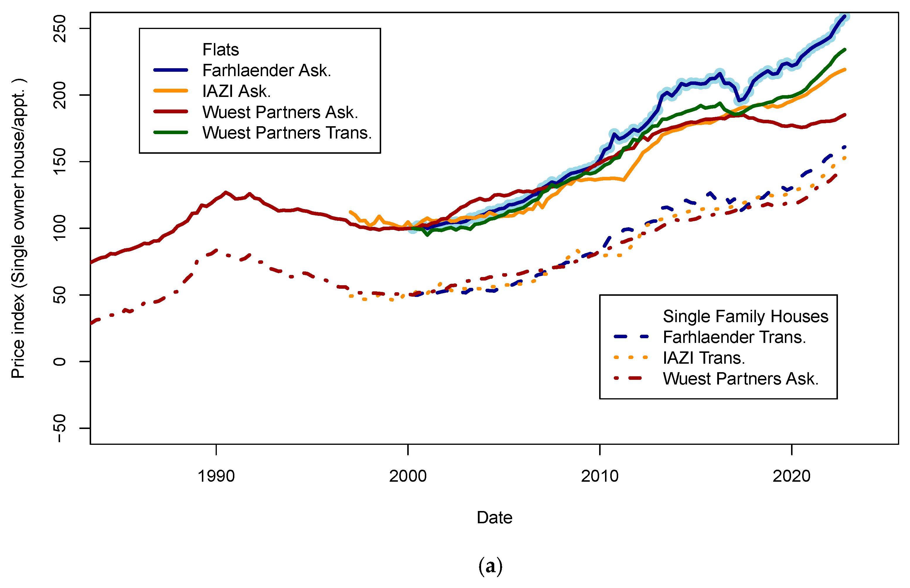
Figure 1.
Real estate prices as published on the SNB data portal. (
a) Ask and transaction prices for flats and single-family houses in Switzerland. Prices for single-family houses have been shifted by minus 50 points for visibility. It is visible that indices are less scattered for house prices (±5%) than for flats (±15%). Those differences may be explained by various reasons, such as geographic sampling, range of asset quality, etc. (
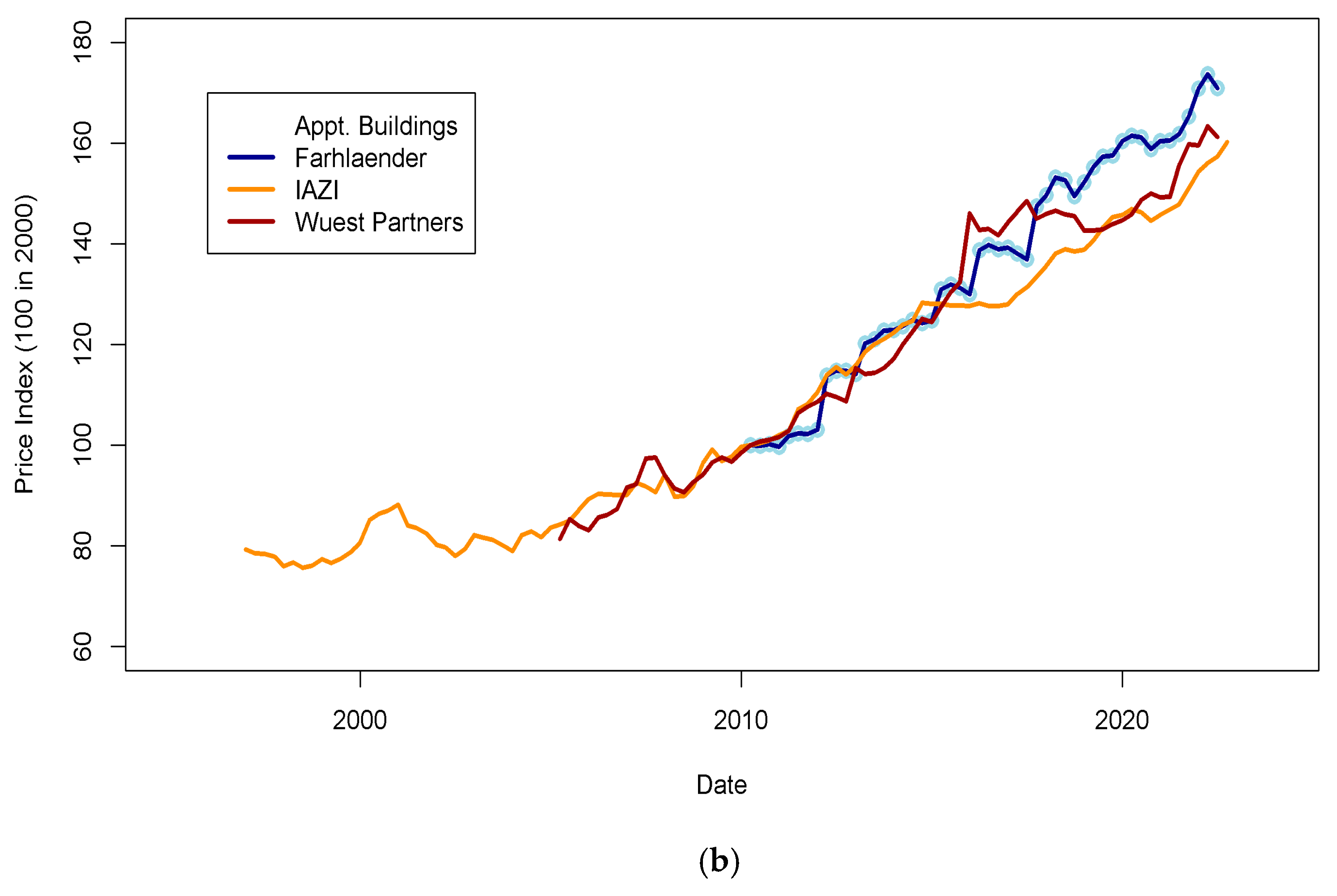
b) Transaction prices for apartment buildings in Switzerland in different indices. The standard deviation of index prices is close to ±5%. Data sources: IAZI (
https://www.iazicifi.ch/, accessed on 6 January 2023), Wuest Partners (
https://www.wuestpartner.com/ch-en/, accessed on 6 January 2023) and Fahrlender (
https://en.fpre.ch/, accessed on 6 January 2023).
Figure 1.
Real estate prices as published on the SNB data portal. (
a) Ask and transaction prices for flats and single-family houses in Switzerland. Prices for single-family houses have been shifted by minus 50 points for visibility. It is visible that indices are less scattered for house prices (±5%) than for flats (±15%). Those differences may be explained by various reasons, such as geographic sampling, range of asset quality, etc. (
b) Transaction prices for apartment buildings in Switzerland in different indices. The standard deviation of index prices is close to ±5%. Data sources: IAZI (
https://www.iazicifi.ch/, accessed on 6 January 2023), Wuest Partners (
https://www.wuestpartner.com/ch-en/, accessed on 6 January 2023) and Fahrlender (
https://en.fpre.ch/, accessed on 6 January 2023).
Figure 2.
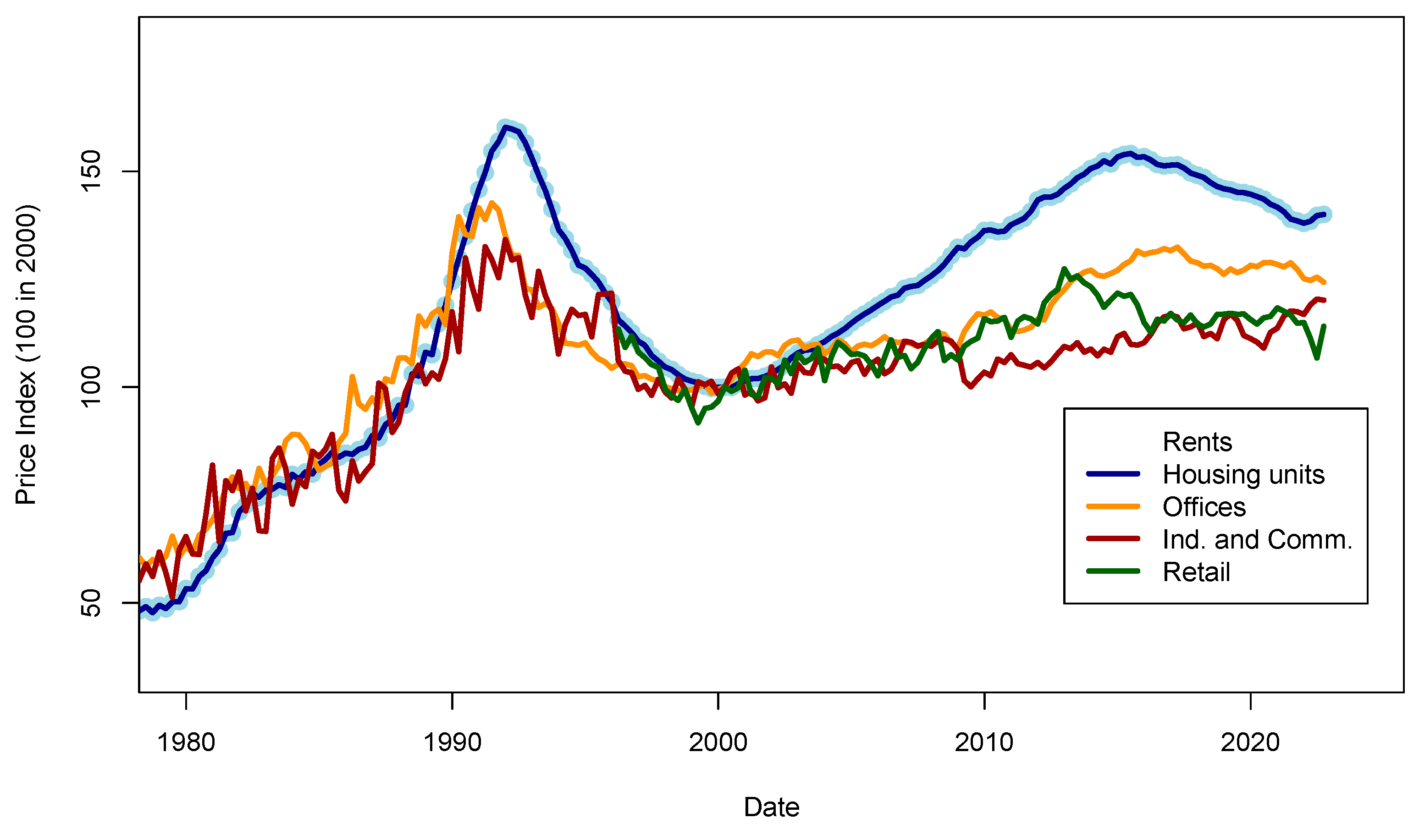
Rent level series for various non-occupied assets. Data source: Swiss National Bank. The final model of this study will include the rent level for housing units (flats and single-family houses). The rent model evolution follows well the evolution of prices, at least until 2015. Further analysis may be necessary to understand why rents were decreasing in the years 2015–2020 while buy prices kept increasing.
Figure 2.
Rent level series for various non-occupied assets. Data source: Swiss National Bank. The final model of this study will include the rent level for housing units (flats and single-family houses). The rent model evolution follows well the evolution of prices, at least until 2015. Further analysis may be necessary to understand why rents were decreasing in the years 2015–2020 while buy prices kept increasing.
Figure 3.
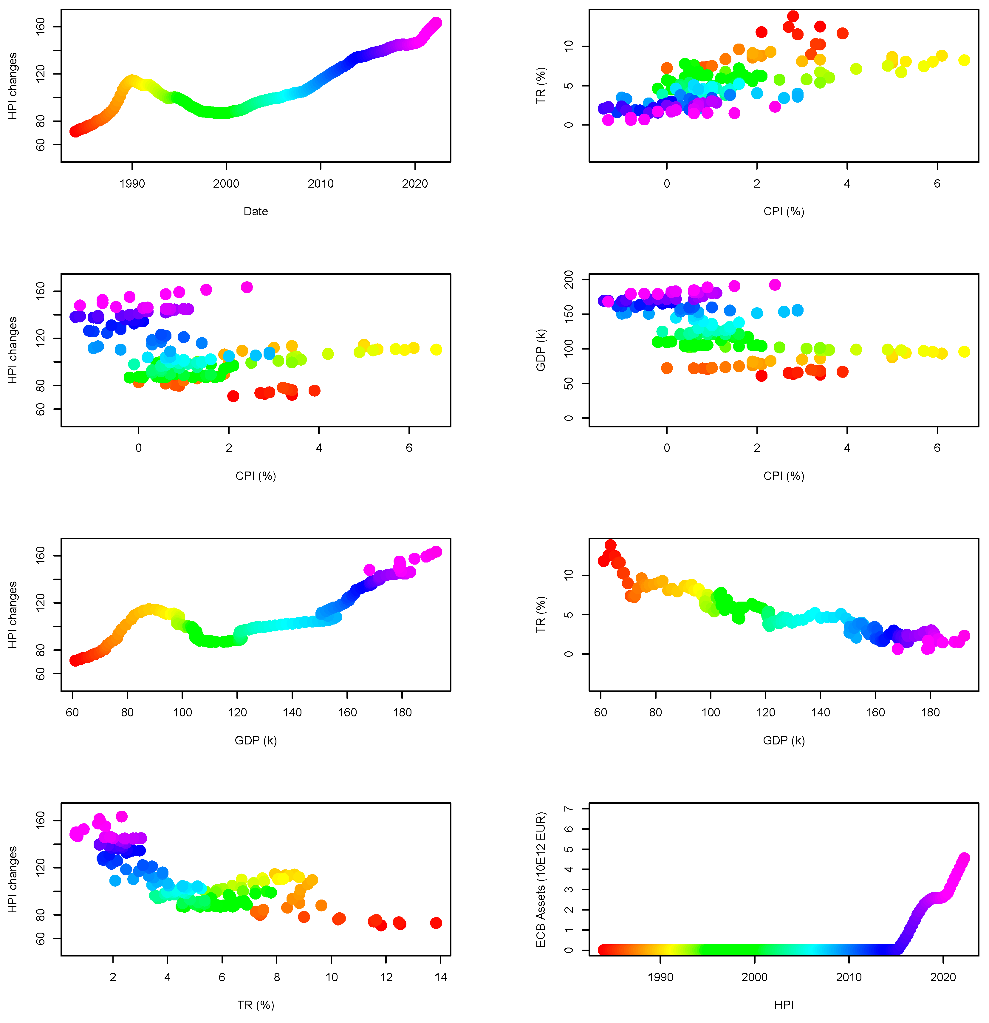
Evolution of economic variables in Switzerland. Inflation seems to be correlated to prices only over the long-term. From the analysis of the GDP series, prices seem to evolve independently of it. Finally, US Treasury rates, if they are correlated to prices, seem to vary by many percent points without impacting the prices. Sources are the FRED database and HPI dataset. The color code consistently symbolizes the date of each point across the panels (see first panel to obtain the correspondence between dates and color code).
Figure 3.
Evolution of economic variables in Switzerland. Inflation seems to be correlated to prices only over the long-term. From the analysis of the GDP series, prices seem to evolve independently of it. Finally, US Treasury rates, if they are correlated to prices, seem to vary by many percent points without impacting the prices. Sources are the FRED database and HPI dataset. The color code consistently symbolizes the date of each point across the panels (see first panel to obtain the correspondence between dates and color code).
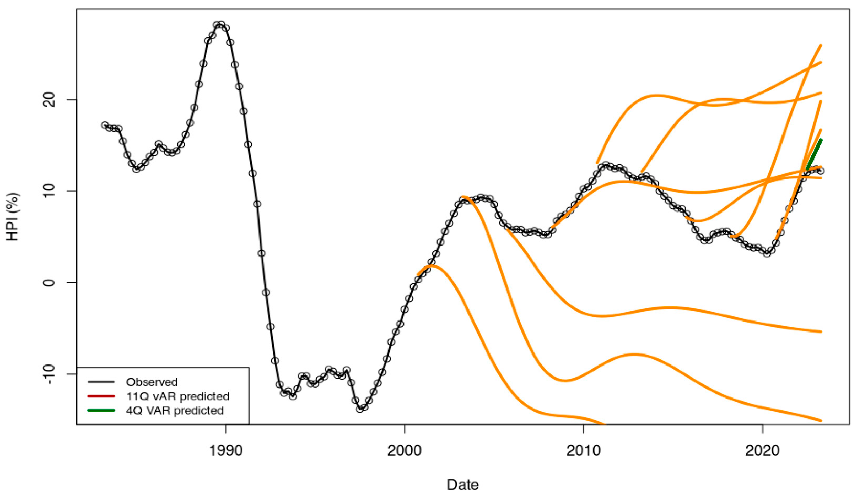
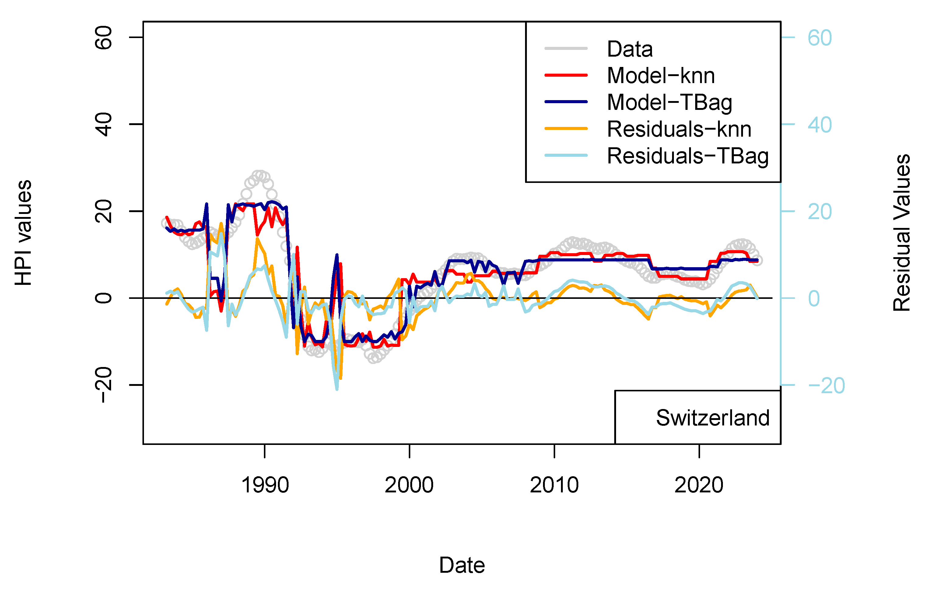
Figure 4.
(
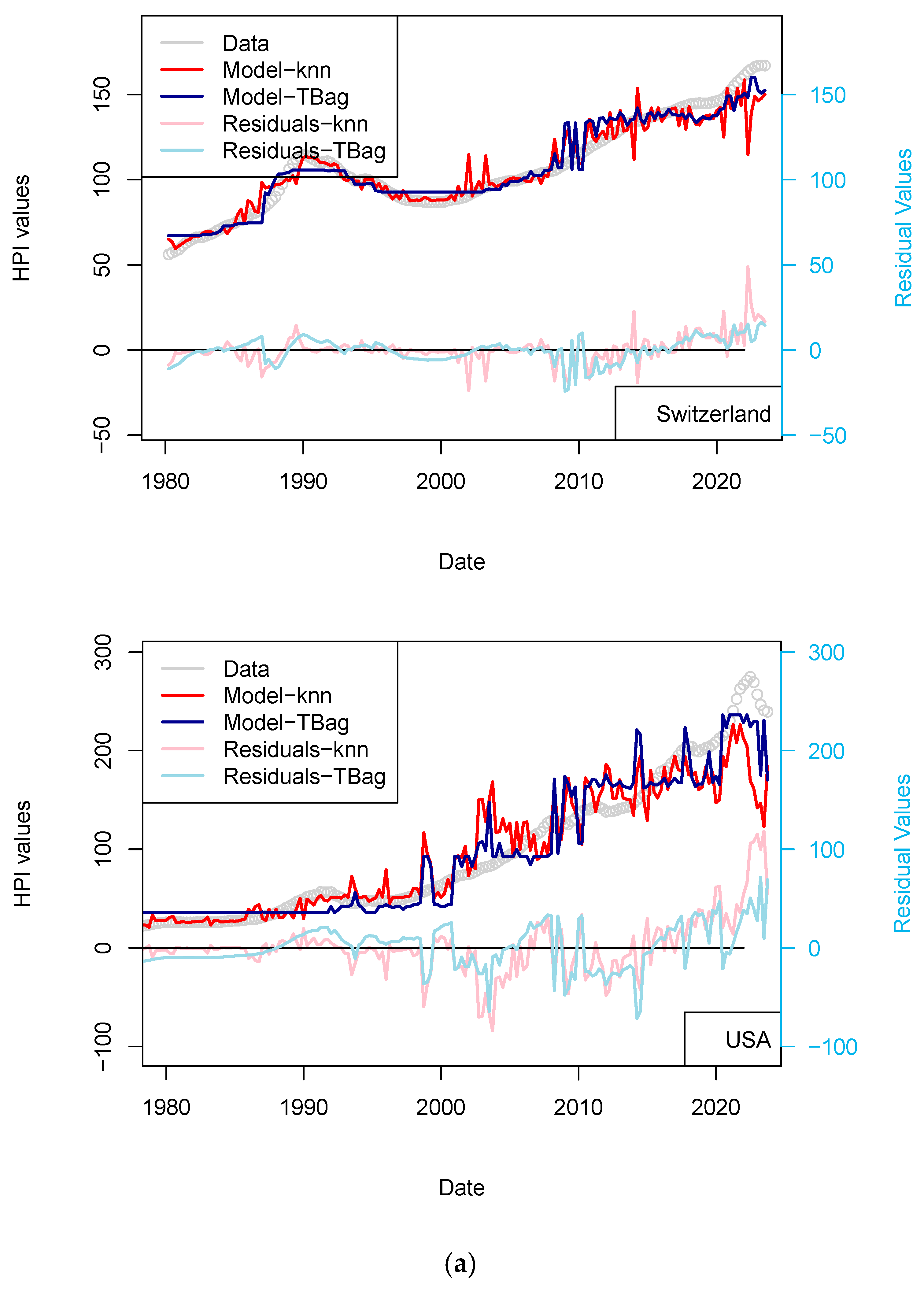
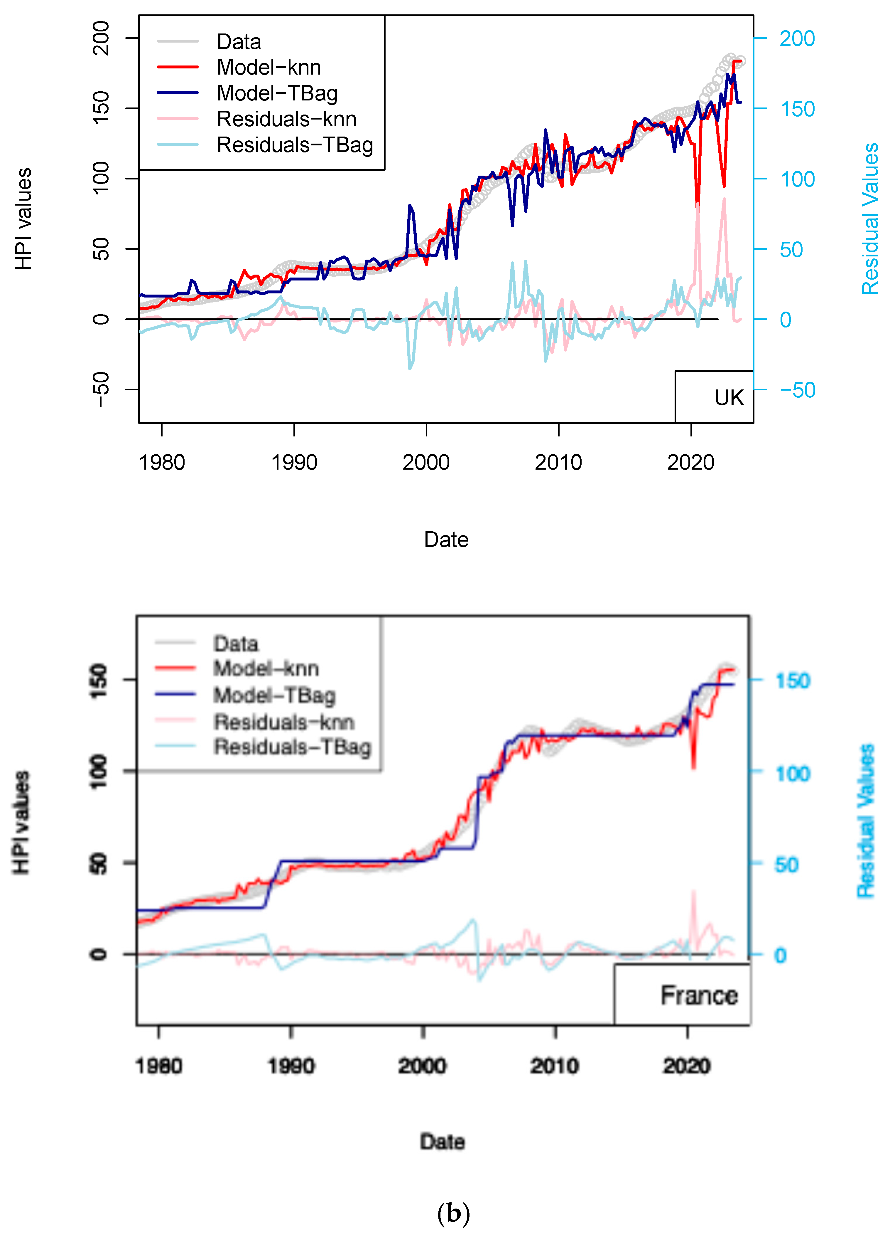
a) “3-param” models. For the sake of presentation, only four countries in the 15 time series modeled are shown in this figure (see the following figure for other results). As explained in the text, most models of this series do not predict an increase in price from 2015 nor during the period following the COVID-19 period. (
b) “3-param” models. For presentation, only four countries of the 15 time series modeled are shown in this figure (see
Supplementary Materials for other results).
Figure 4.
(
a) “3-param” models. For the sake of presentation, only four countries in the 15 time series modeled are shown in this figure (see the following figure for other results). As explained in the text, most models of this series do not predict an increase in price from 2015 nor during the period following the COVID-19 period. (
b) “3-param” models. For presentation, only four countries of the 15 time series modeled are shown in this figure (see
Supplementary Materials for other results).
Figure 5.
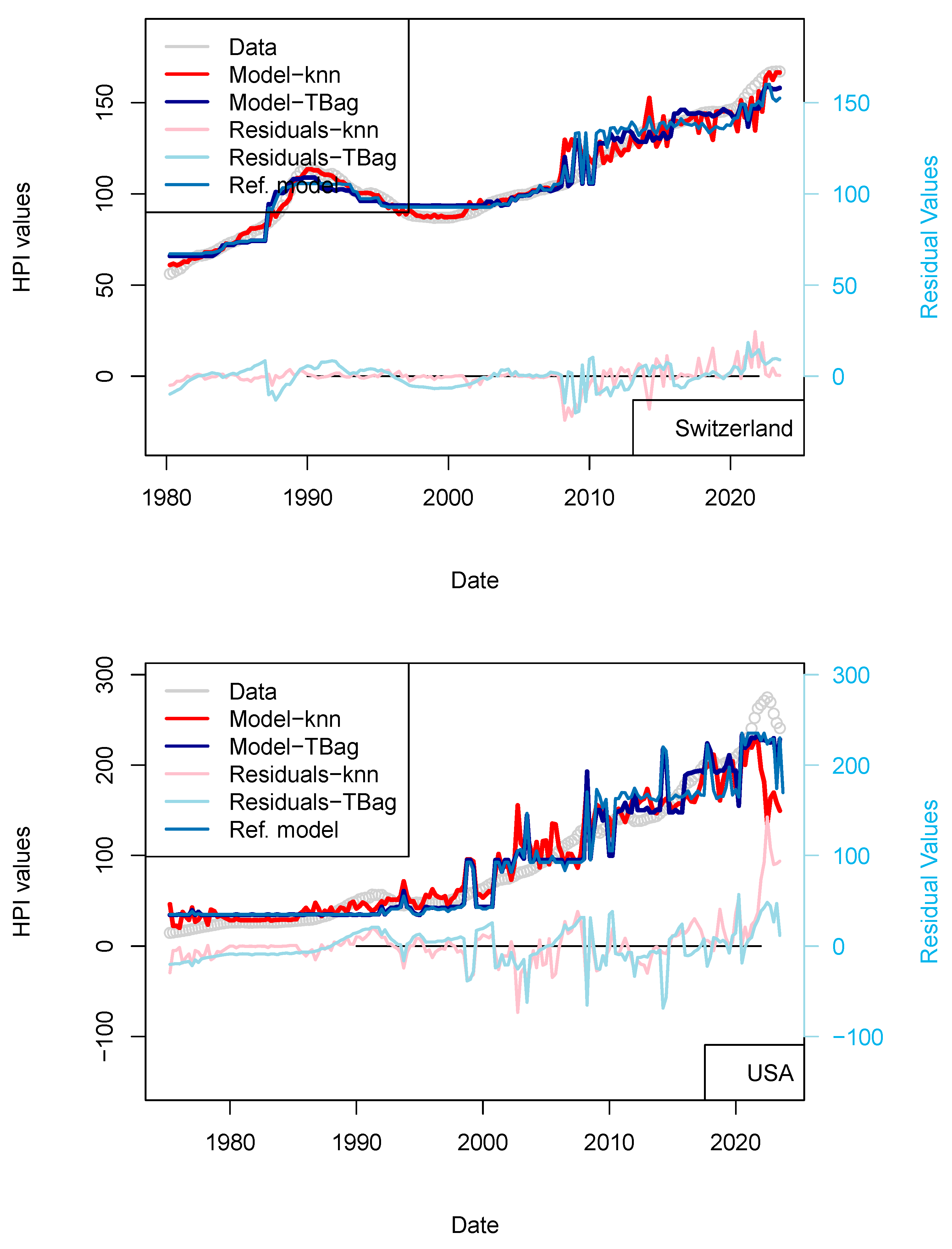
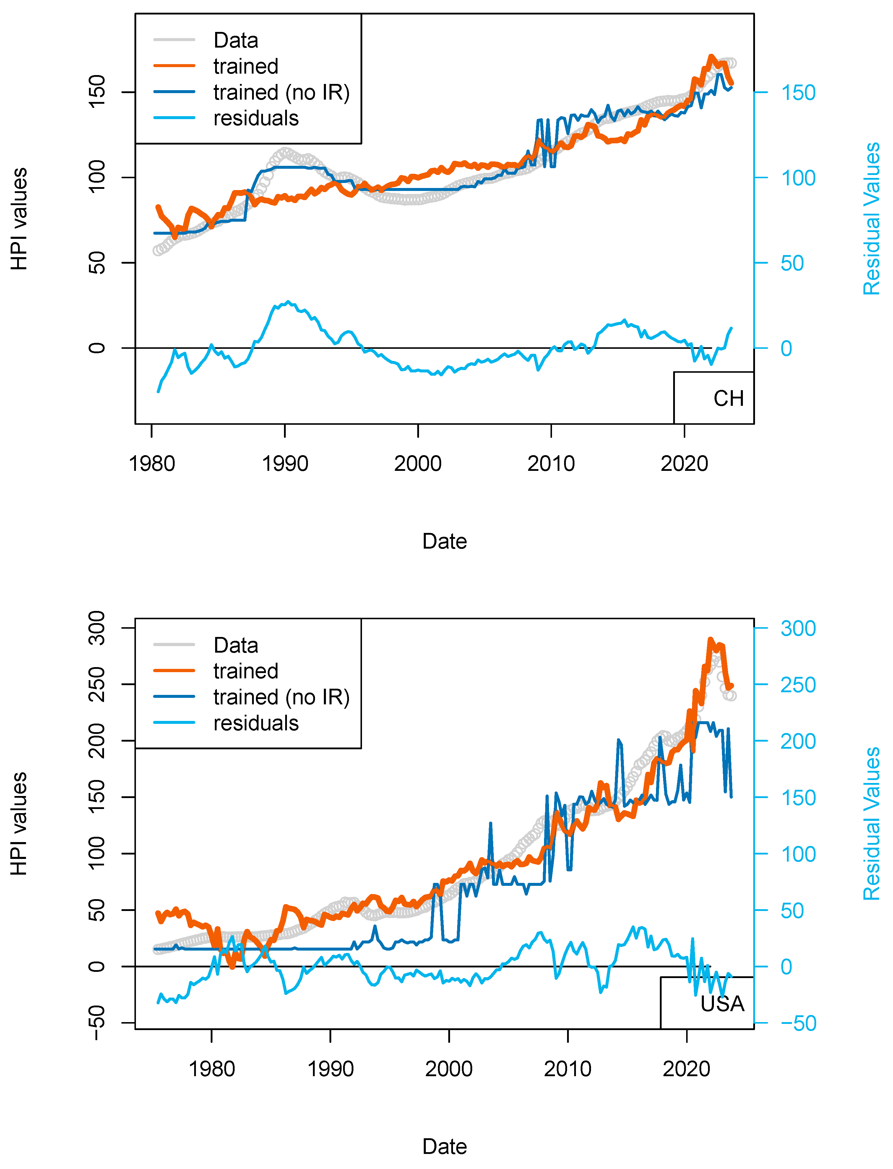
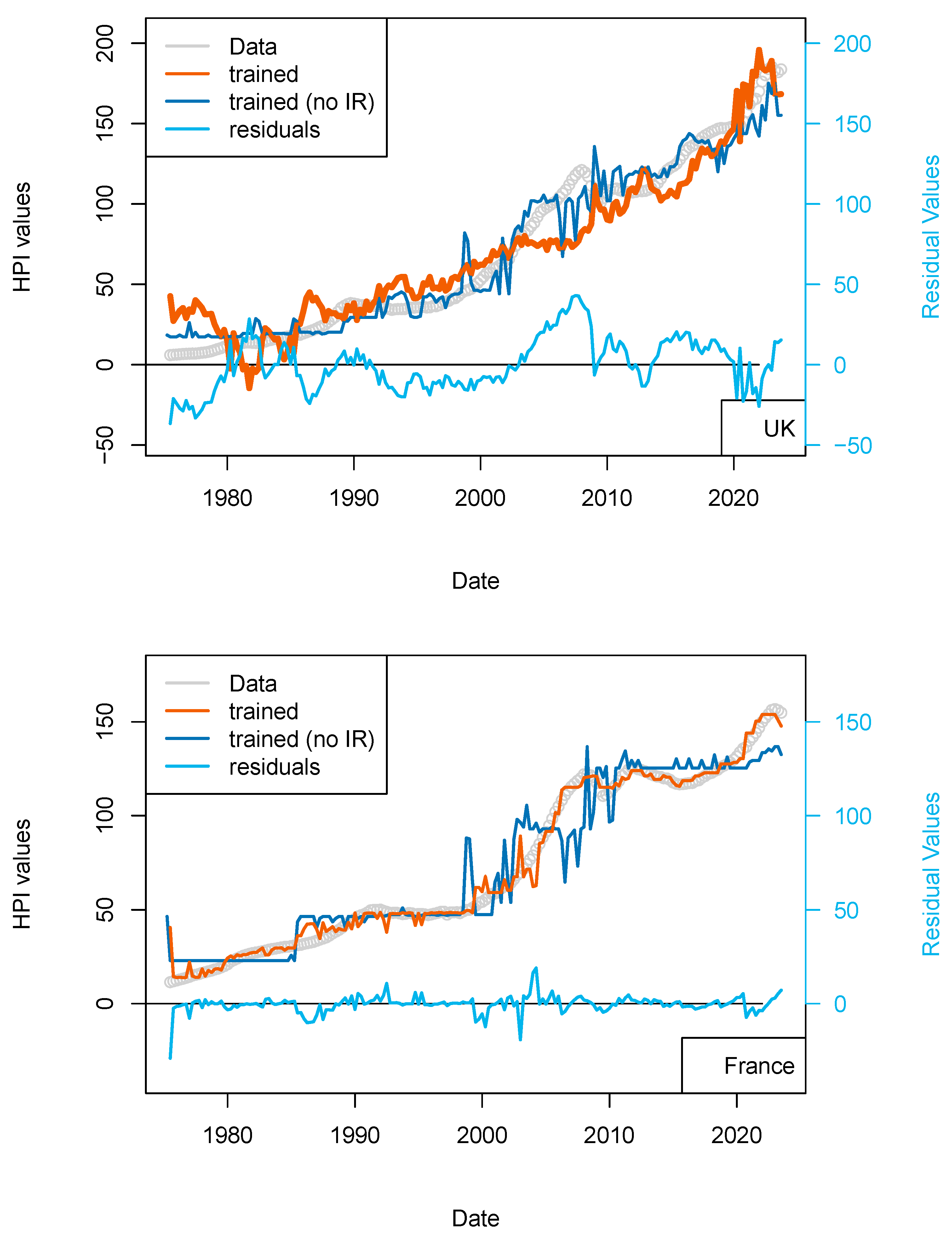
“Central bank IR” models. Comparison of models including (or not) the US FED interest rates to all countries. Parameters used here are CPI, GDP, and treasury rates (10-yr), and for one of the two models, the Swiss National Bank (SNB) interest rates. The price history modeled without using the central bank rates is shown using a blue curve. All models benefit from including the interest rates (see all orange curves).
Figure 5.
“Central bank IR” models. Comparison of models including (or not) the US FED interest rates to all countries. Parameters used here are CPI, GDP, and treasury rates (10-yr), and for one of the two models, the Swiss National Bank (SNB) interest rates. The price history modeled without using the central bank rates is shown using a blue curve. All models benefit from including the interest rates (see all orange curves).
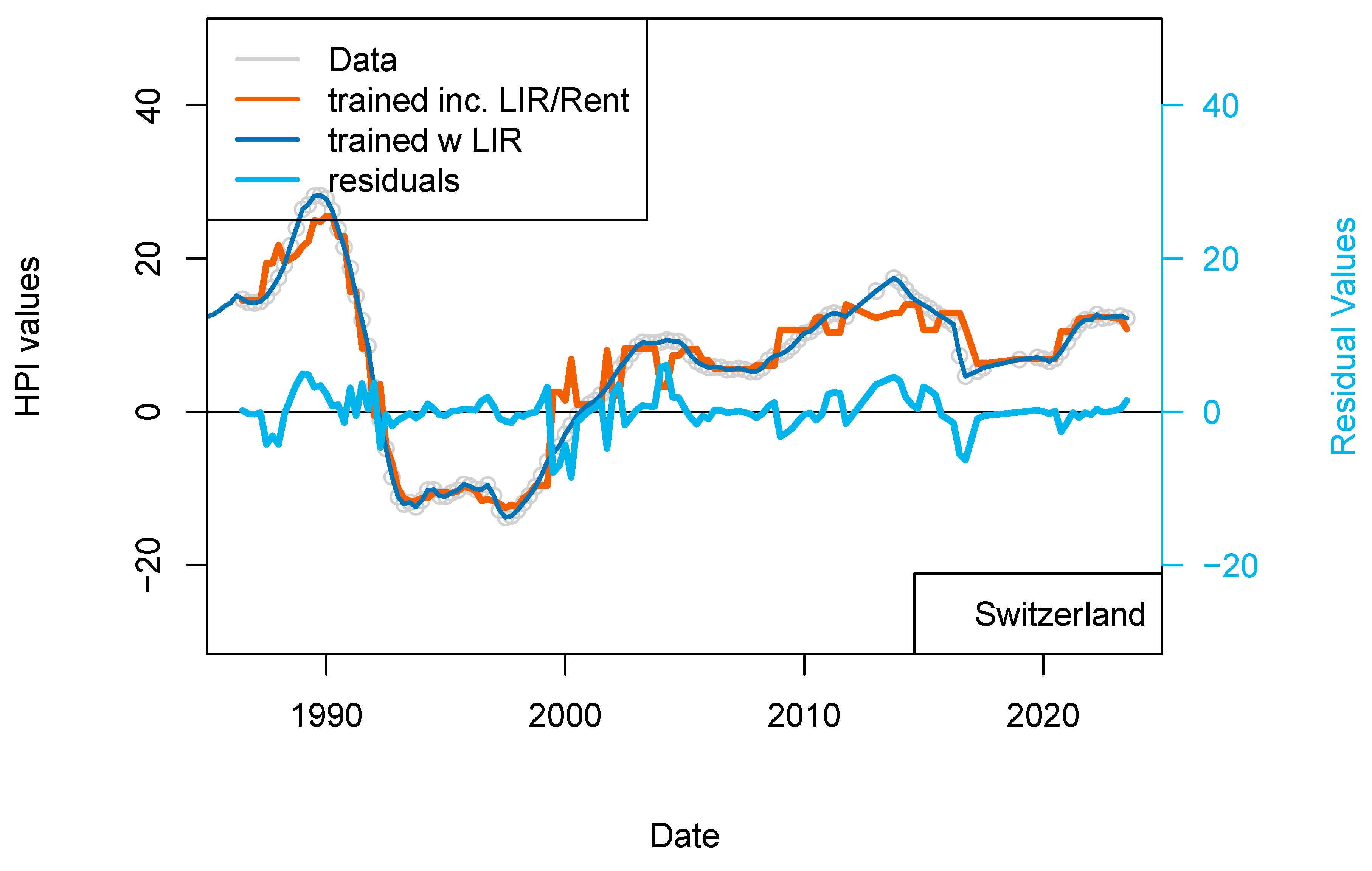
Figure 6.
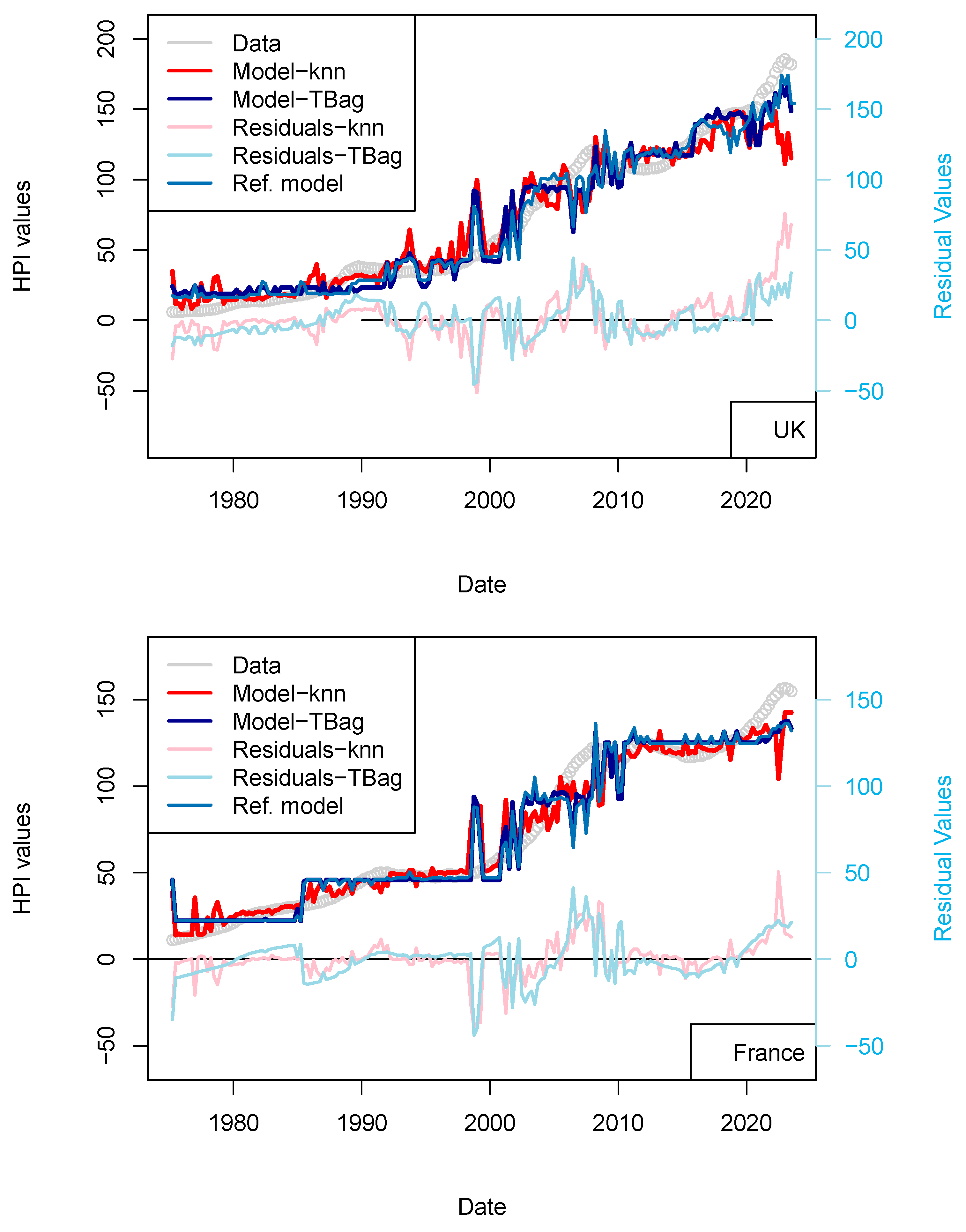
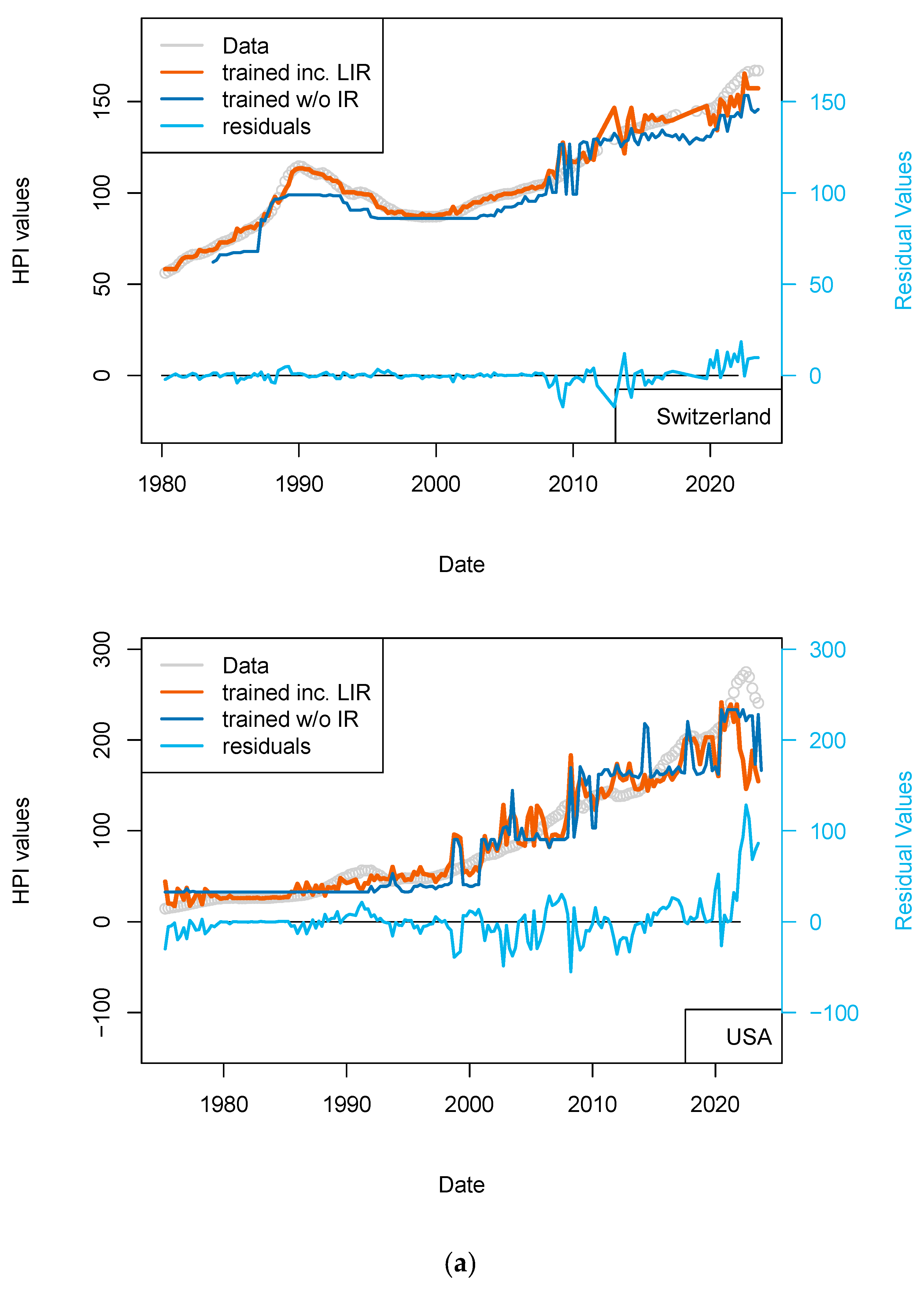
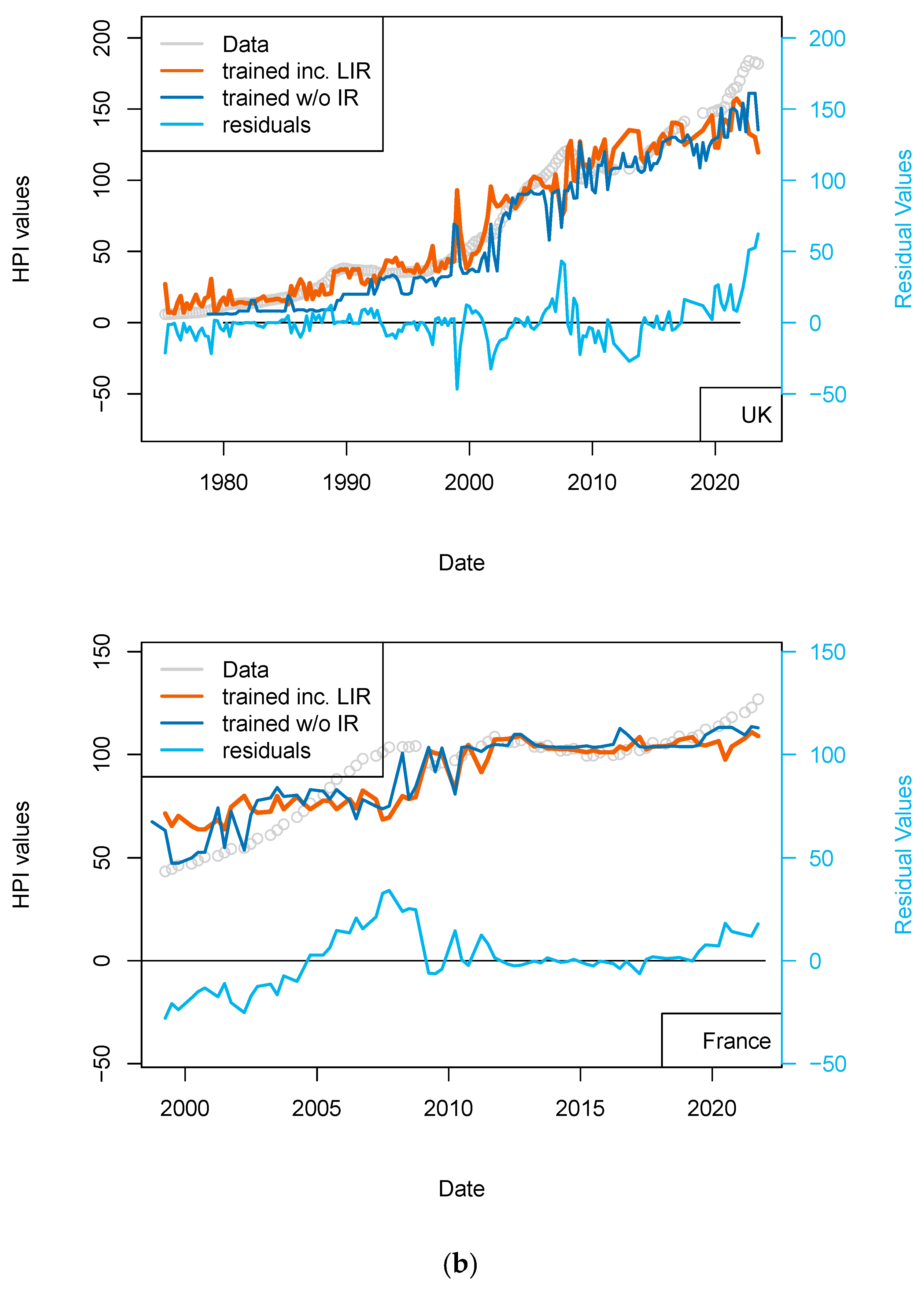
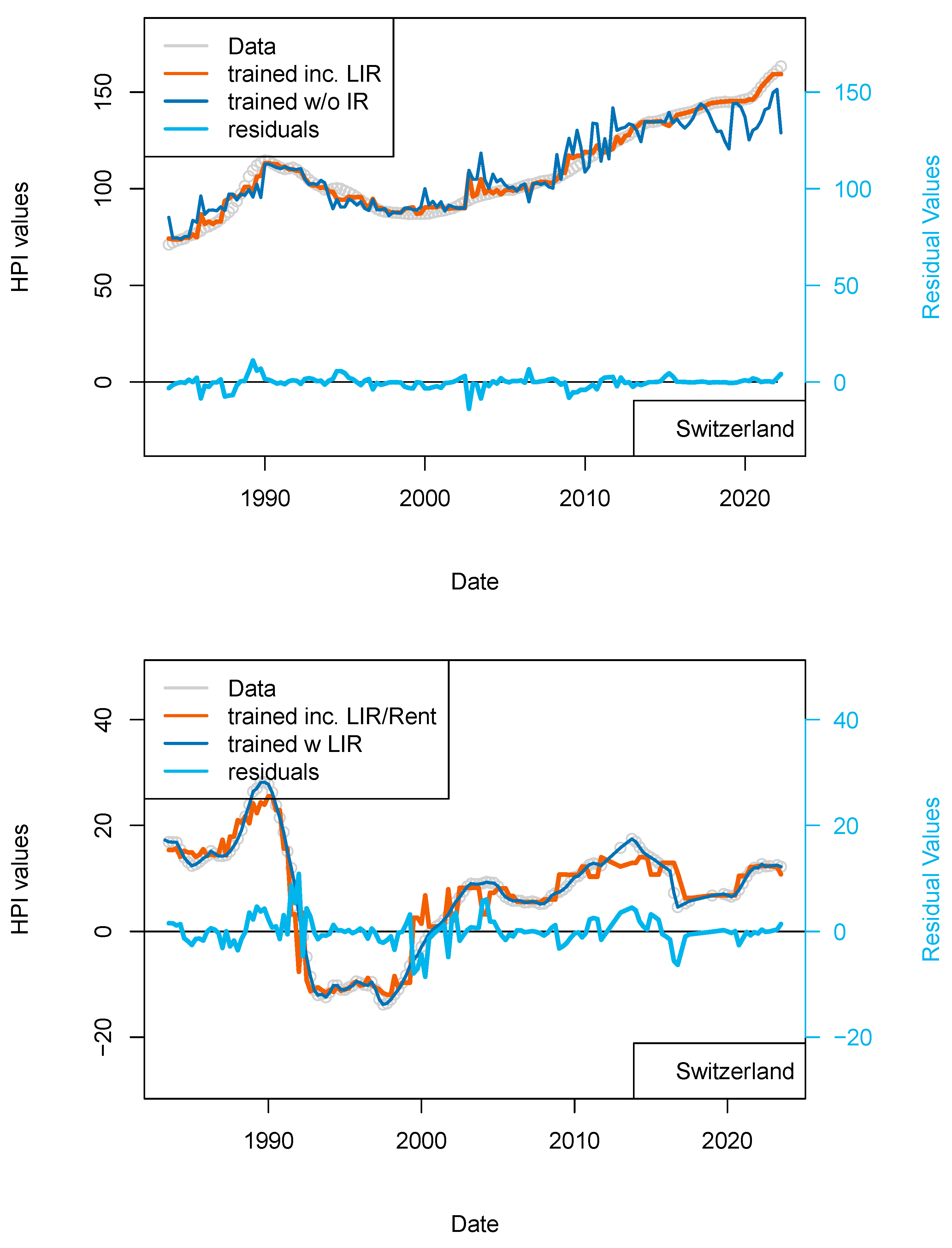
(a) “LIR” model. Comparison of models including (or not) the US FED interest rates to all countries, unless some local rates are available (CH, EU rates). Parameters used here are CPI, GDP, and treasury rates (10-yr), and for one of the two models, the Swiss National Bank (SNB) interest rates. The price history modeled without using the central bank rates is shown using a blue curve. All models benefit from including the interest rates (see all orange curves). (b) “LIR” model. Comparison of models including (or not) the US FED interest rates to all countries unless some local rates are available (CH, EU rates). Parameters used here CPI, GDP, treasury rates (10-yr), and for one of the two models, interest rates of Swiss National Bank (SNB). The price history modeled without using the central bank rates is shown using a blue curve. All models benefit from the inclusion of the interest rates (see all orange curves).
Figure 6.
(a) “LIR” model. Comparison of models including (or not) the US FED interest rates to all countries, unless some local rates are available (CH, EU rates). Parameters used here are CPI, GDP, and treasury rates (10-yr), and for one of the two models, the Swiss National Bank (SNB) interest rates. The price history modeled without using the central bank rates is shown using a blue curve. All models benefit from including the interest rates (see all orange curves). (b) “LIR” model. Comparison of models including (or not) the US FED interest rates to all countries unless some local rates are available (CH, EU rates). Parameters used here CPI, GDP, treasury rates (10-yr), and for one of the two models, interest rates of Swiss National Bank (SNB). The price history modeled without using the central bank rates is shown using a blue curve. All models benefit from the inclusion of the interest rates (see all orange curves).
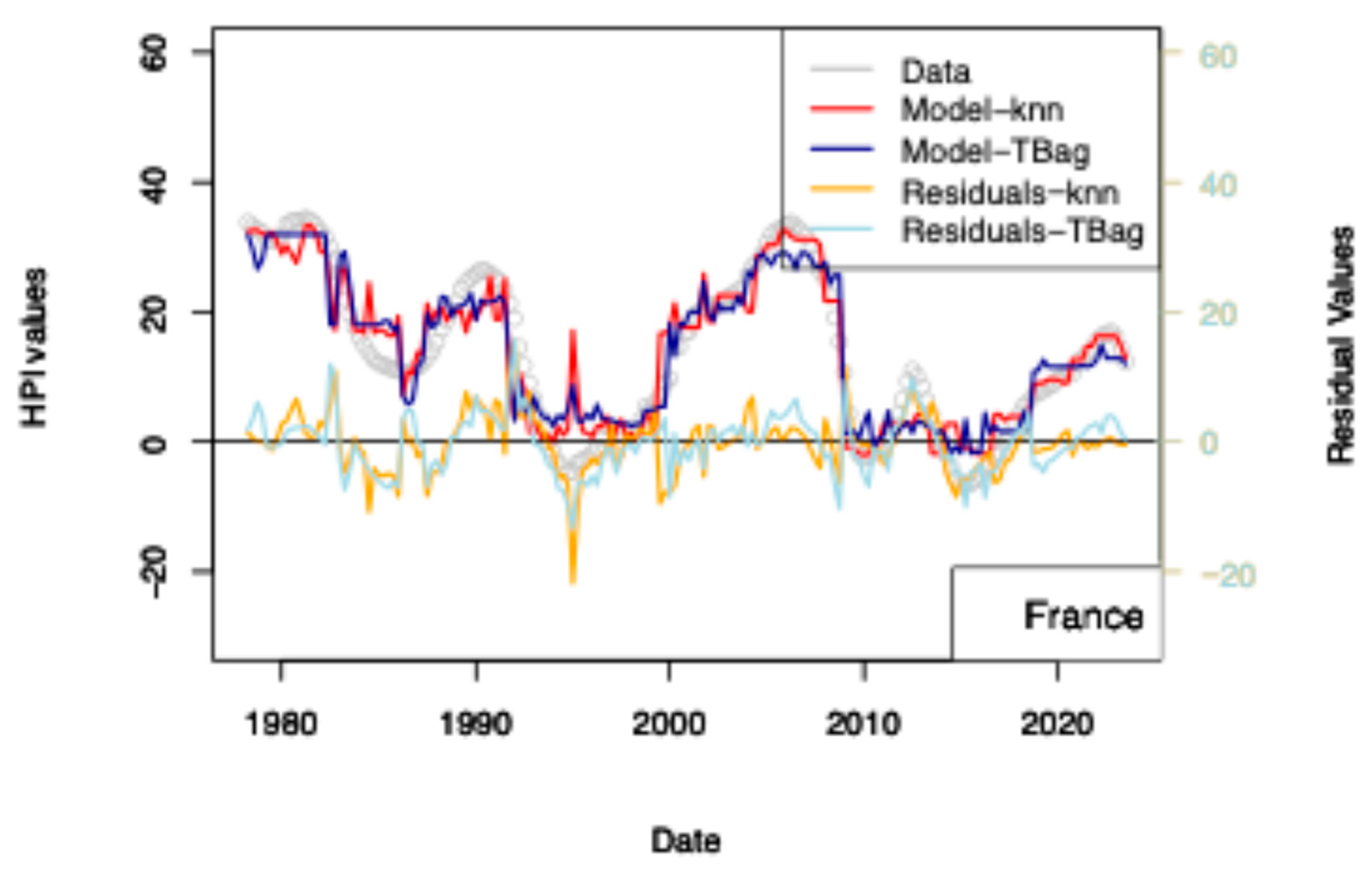
Figure 7.
“ECB” model. With the exception of France, all the four time-series fits benefit from the addition of the ECB purchase data. One explanation of this difference could be that, in France, the amortization of the asset is complete over the period of the loan. As, in combination, most loans are on fixed rates, shocks to interest rates therefore have less of a pronounced impact on the market.
Figure 8.
“ECB/FED” models: Effect of the inclusion of the data of ECB PSPP/PEPP programs and of FED Quantitative Easing (QE) programs (FED total asset book size). The data (grey) and the ECB+FED model (orange) are compared with the 3-param model.
Figure 8.
“ECB/FED” models: Effect of the inclusion of the data of ECB PSPP/PEPP programs and of FED Quantitative Easing (QE) programs (FED total asset book size). The data (grey) and the ECB+FED model (orange) are compared with the 3-param model.
Figure 9.
(top) “Rents” model. Results of the dataset including the rent level for Switzerland. Rent levels date back to 1939 (base 100) and have been differentiated. (bottom) “Rent_1 yr model”. Comparison of the model including PSPP, SNB interest rates and rent levels for Switzerland (orange) with the model including only TR, IR, GDP and inflation (dark blue). This figure suggests some level of overfitting of the first versions of the model.
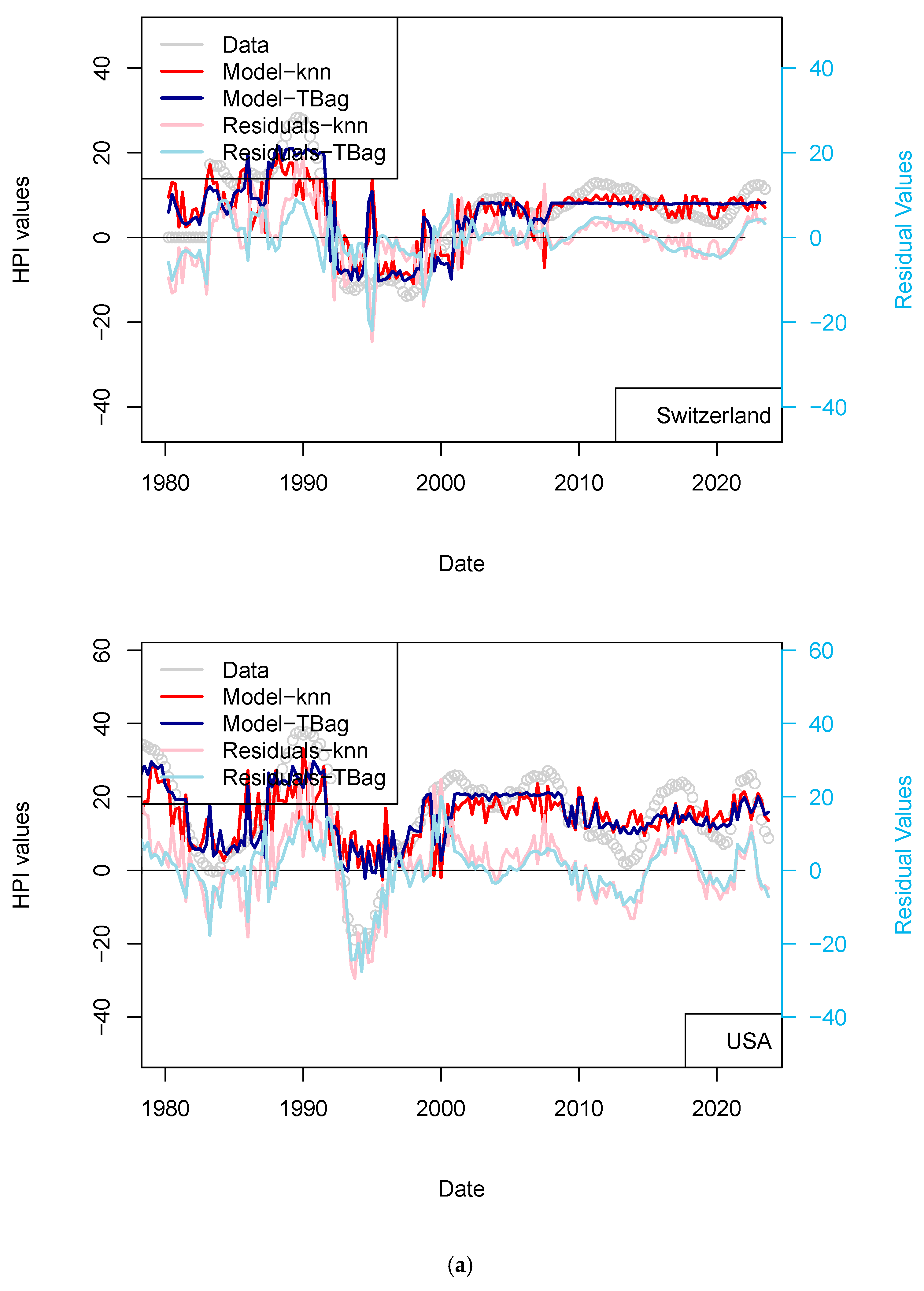
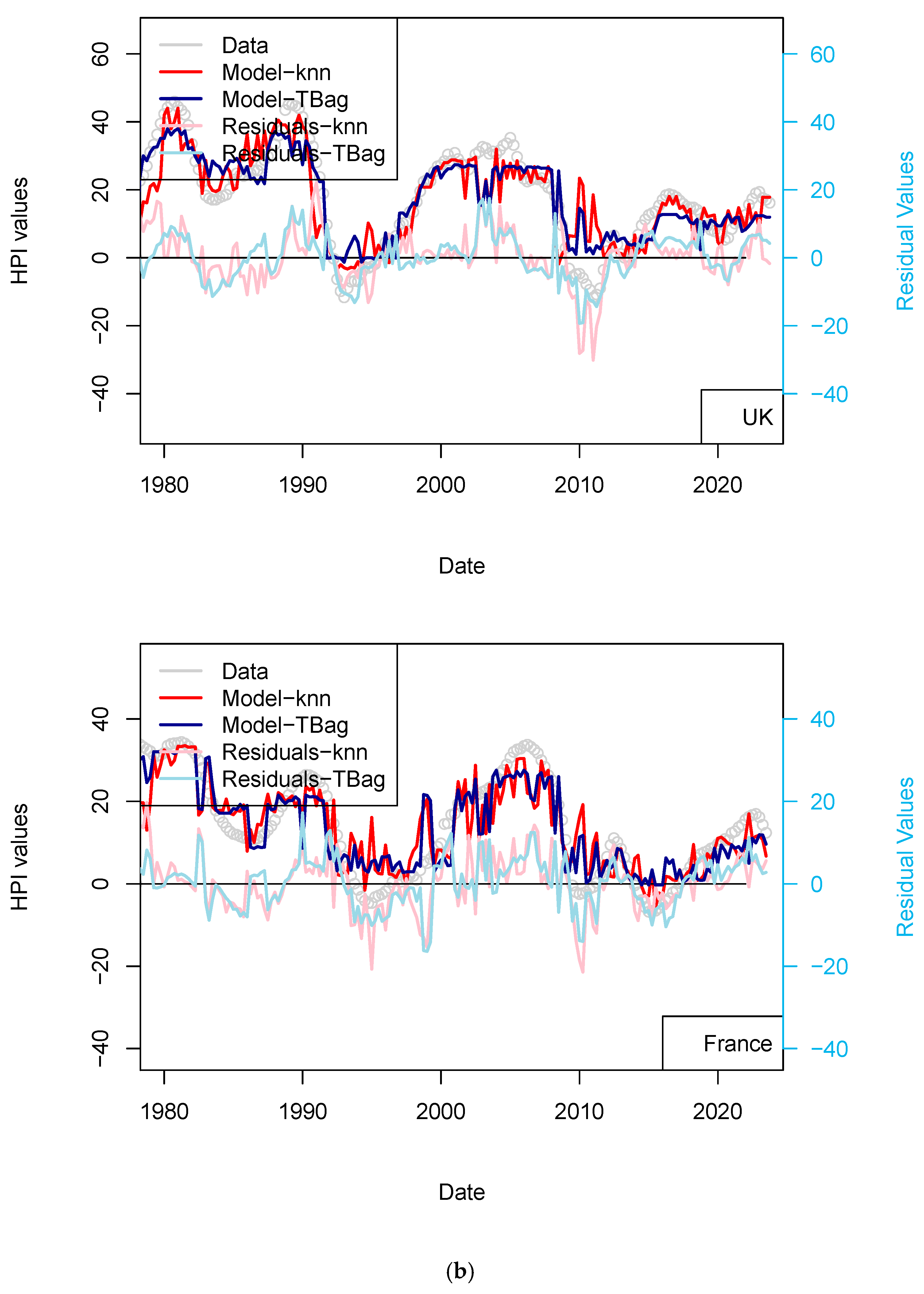
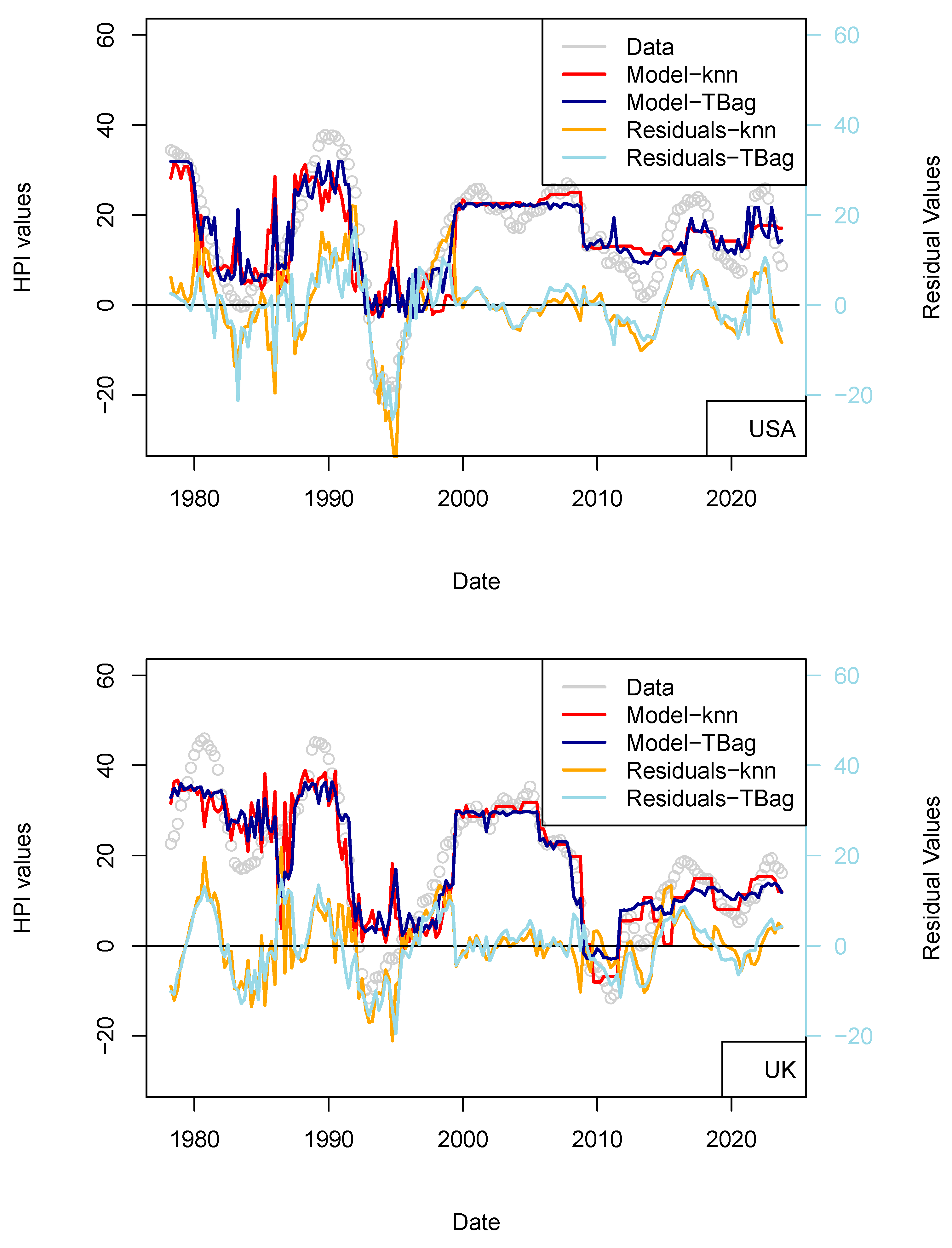
Figure 10.
(
a) “3-param 1 yr” Switzerland and USA models. (
b) “3-param 1 yr” UK and France models. Input data are the same as those used for the model presented in
Figure 4. HPIs are differentiated over 12 quarters.
Figure 10.
(
a) “3-param 1 yr” Switzerland and USA models. (
b) “3-param 1 yr” UK and France models. Input data are the same as those used for the model presented in
Figure 4. HPIs are differentiated over 12 quarters.
Figure 11.
ECB 1 yr model. Input data are the same as those used for the model presented in
Figure 7. HPIs are differentiated over 12 quarters.
Figure 11.
ECB 1 yr model. Input data are the same as those used for the model presented in
Figure 7. HPIs are differentiated over 12 quarters.
Figure 12.
“Rents 1 yr” model. The model including most of the data discussed in this paper are included in the input dataset (a list of parameters is presented in
Table 8). The performance of the model is compared with the model LIR (GDP, CPI, Treasury rates + central bank rates).
Figure 12.
“Rents 1 yr” model. The model including most of the data discussed in this paper are included in the input dataset (a list of parameters is presented in
Table 8). The performance of the model is compared with the model LIR (GDP, CPI, Treasury rates + central bank rates).
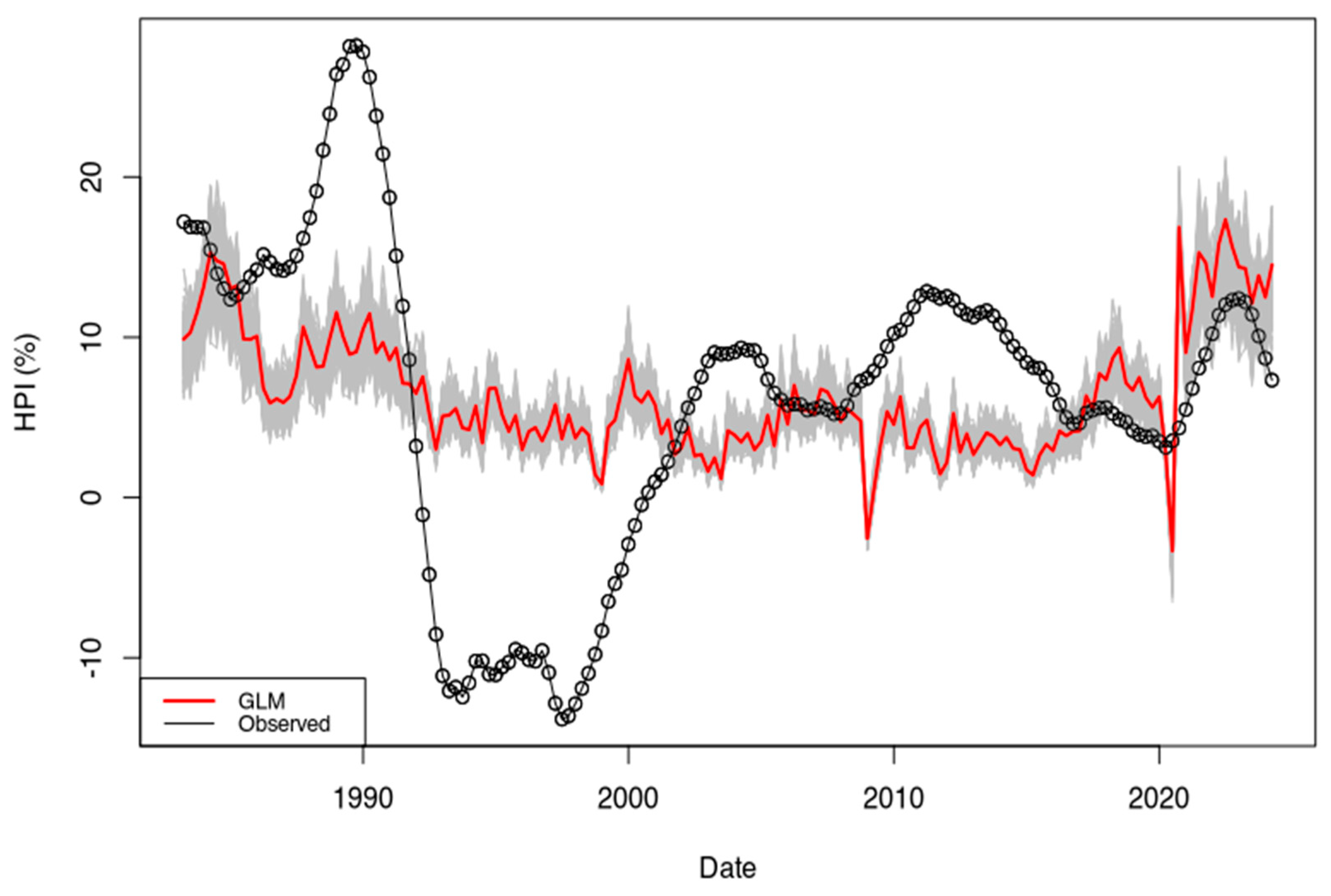
Figure 13.
Comparison of prices for Switzerland (black circles) with prices modeled (dark red) after permuting the input data. This test confirms that the input data chosen are meaningful for modeling HPI and the algorithm is not able to predict prices from noise (overfitting). The “kNN” approach has been used as for other models and tests shown in this paper.
Figure 14.
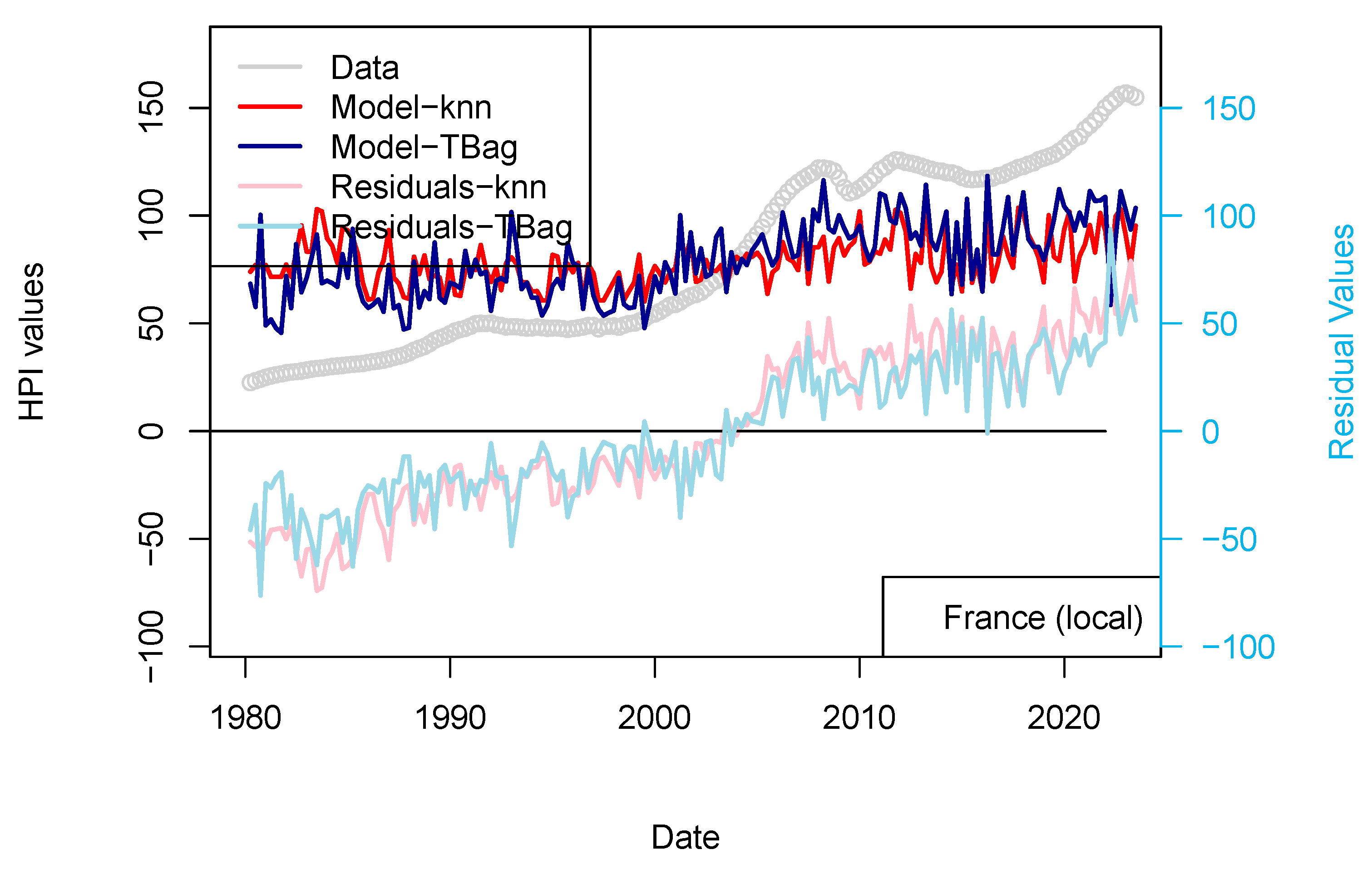
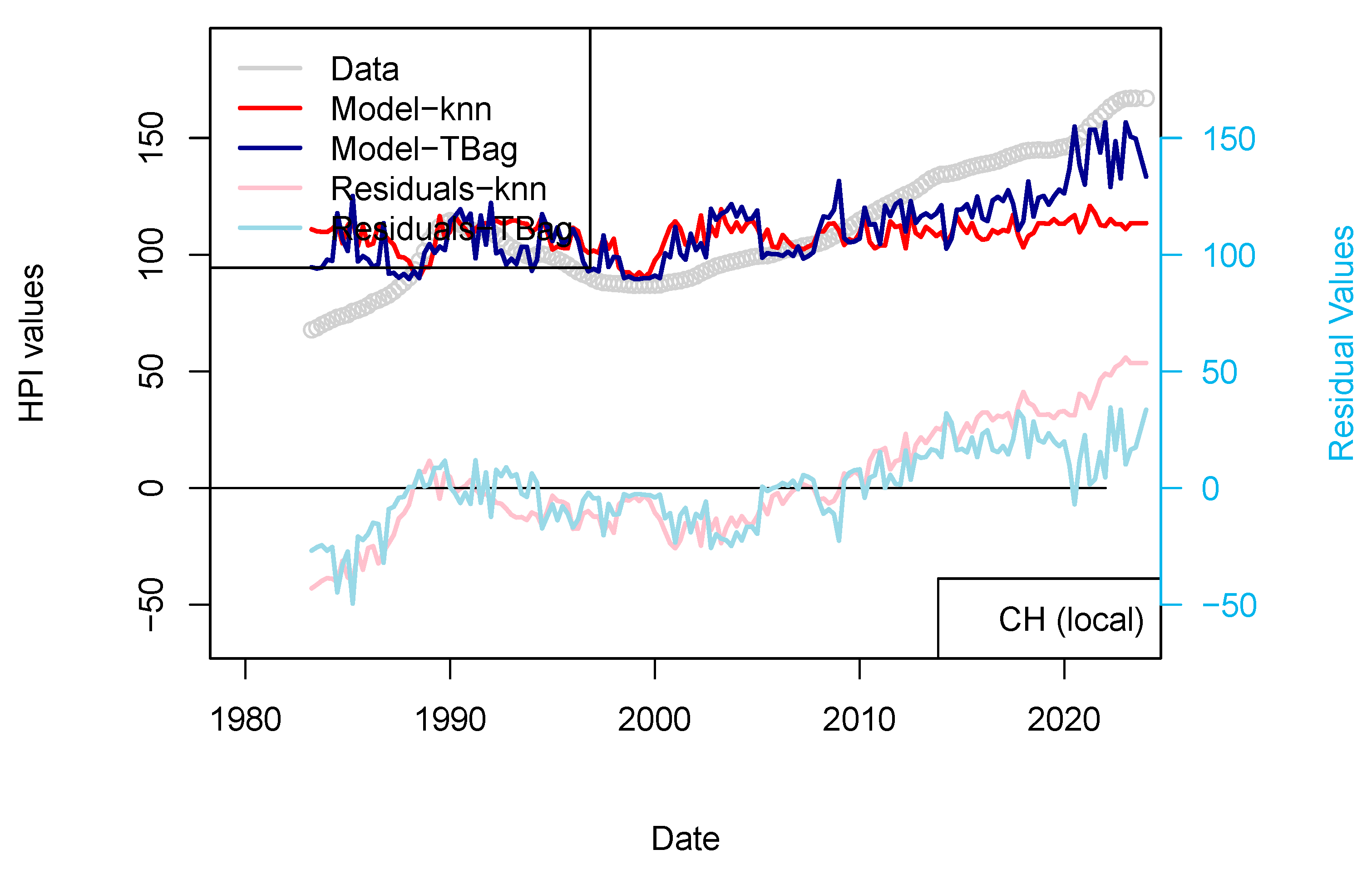
“LOCAL 1 yr” models for France and Switzerland. HPIs are modeled using only local economic factors.
Figure 14.
“LOCAL 1 yr” models for France and Switzerland. HPIs are modeled using only local economic factors.
Figure 15.
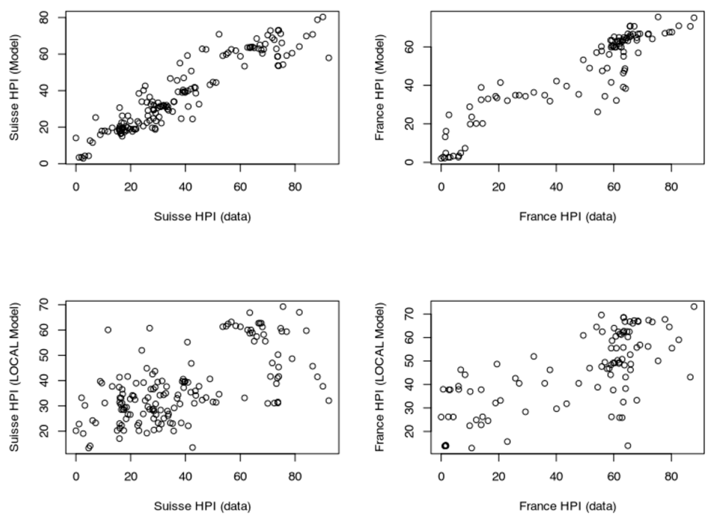
Relative performance of models based on local-only dataset and models including the contribution of treasury rates (for France and Switzerland).
Figure 15.
Relative performance of models based on local-only dataset and models including the contribution of treasury rates (for France and Switzerland).
Figure 16.
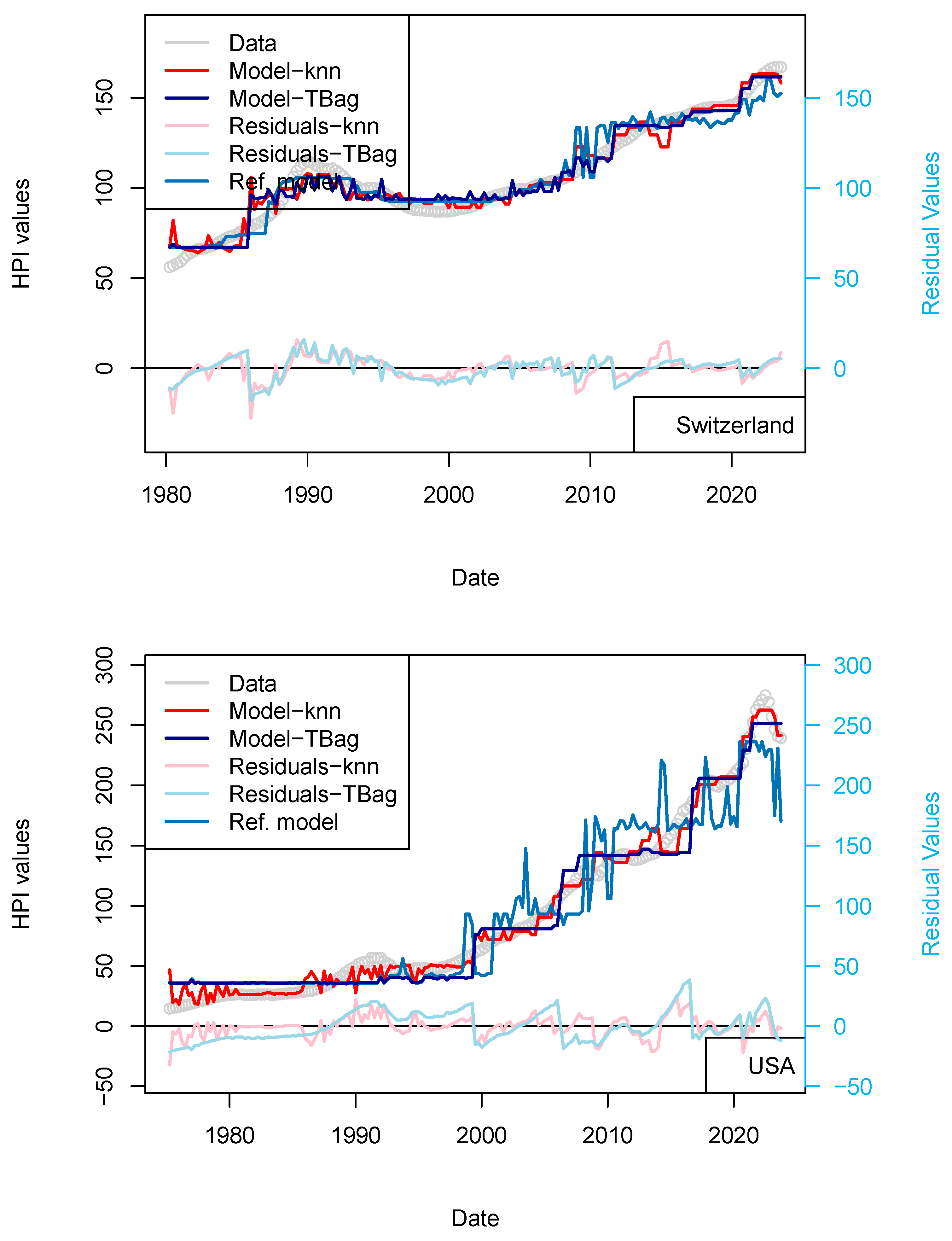
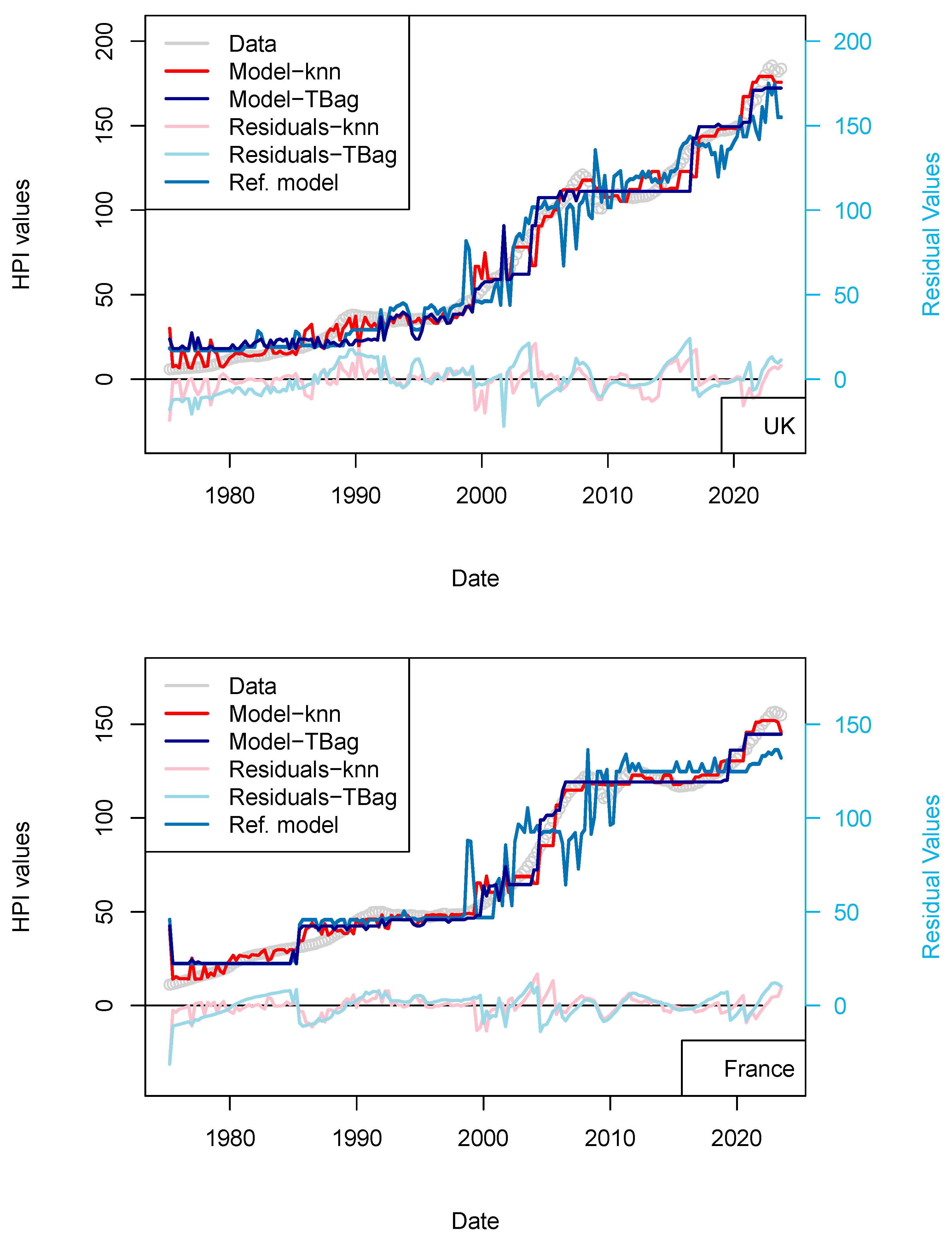
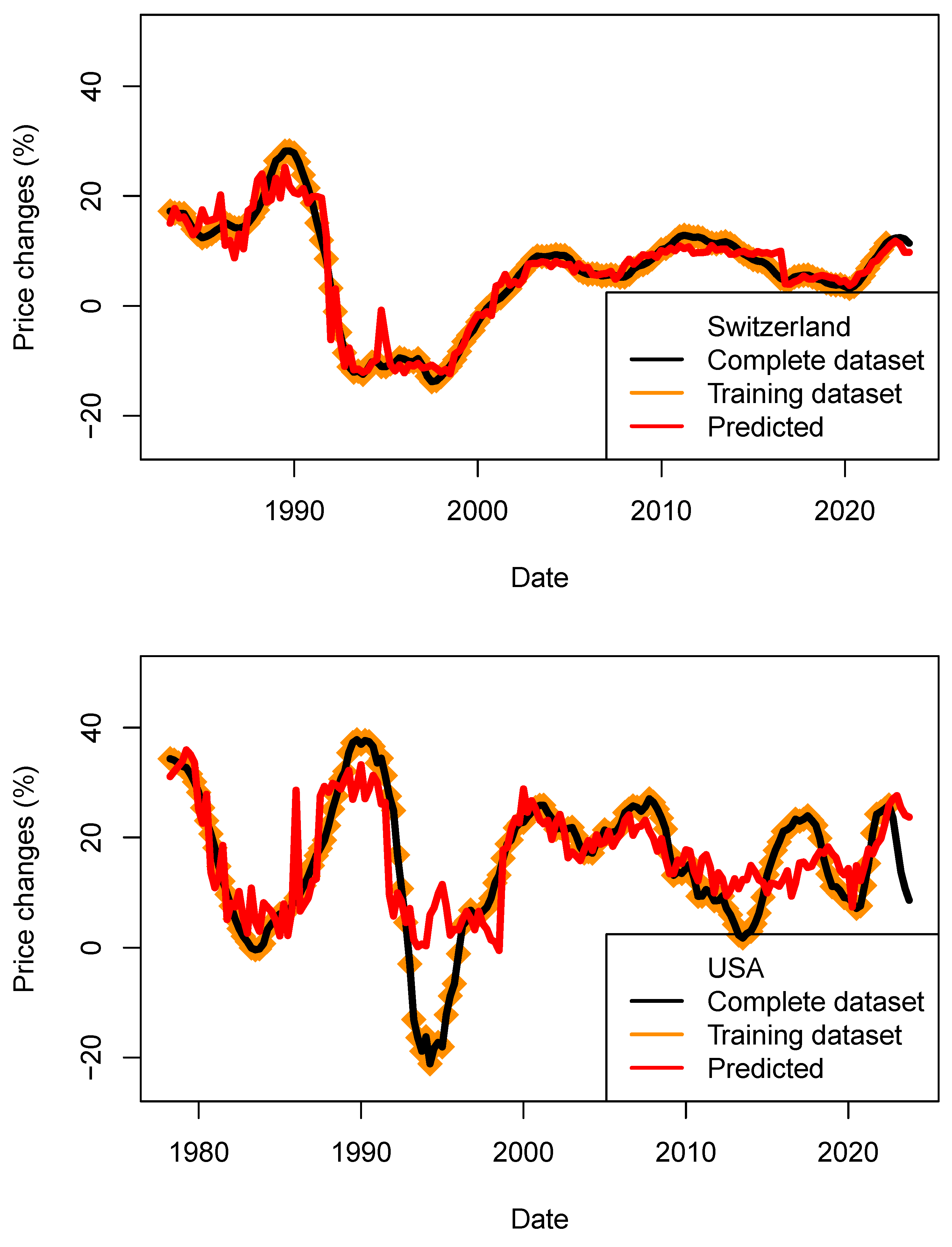
Performance assessment of the price models (ECB_1y_TB_model) for four countries. Predicted price changes are indicated in red, complete dataset in black and training data in orange. For the four countries, price decrease could be modeled.
Figure 16.
Performance assessment of the price models (ECB_1y_TB_model) for four countries. Predicted price changes are indicated in red, complete dataset in black and training data in orange. For the four countries, price decrease could be modeled.
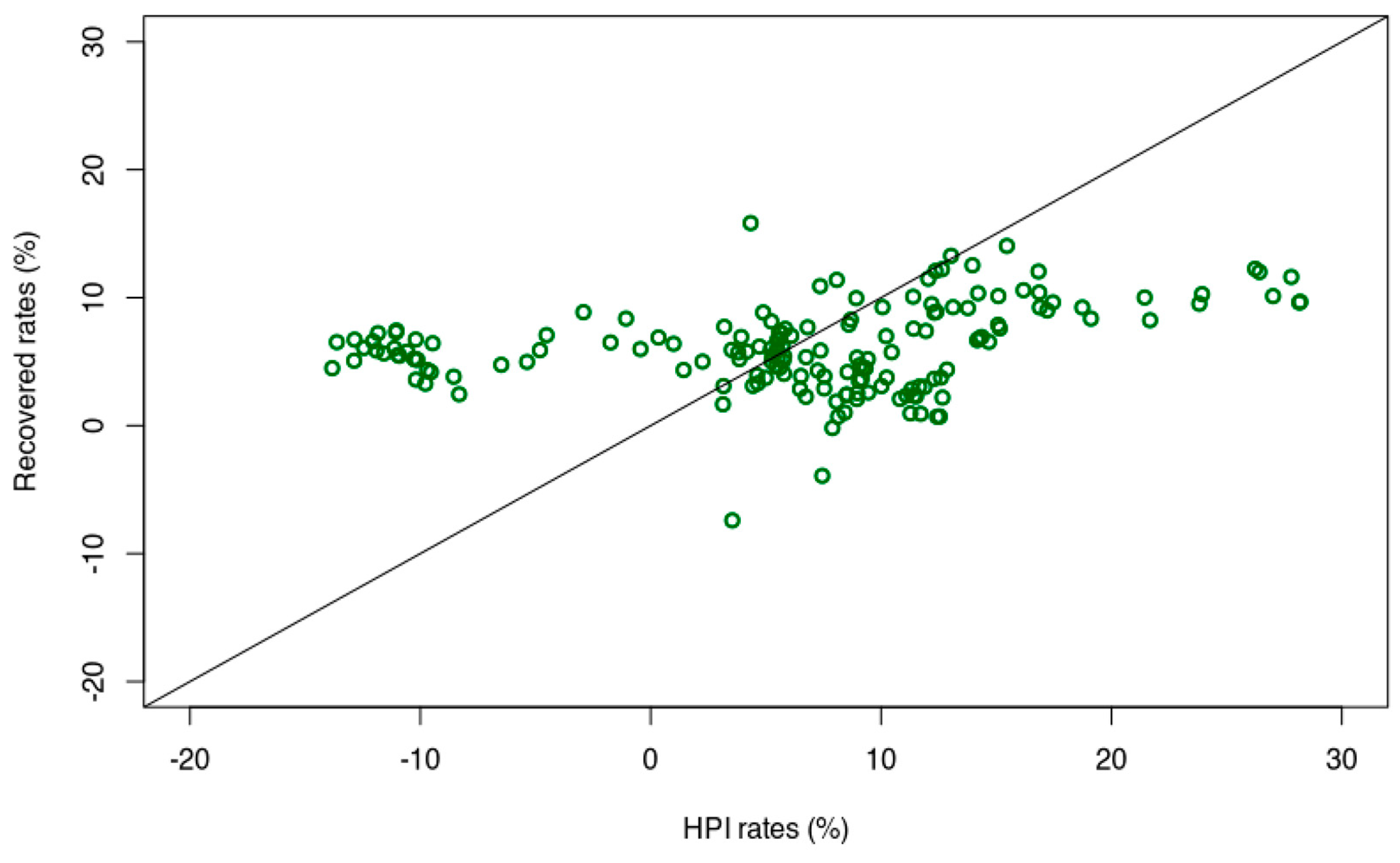
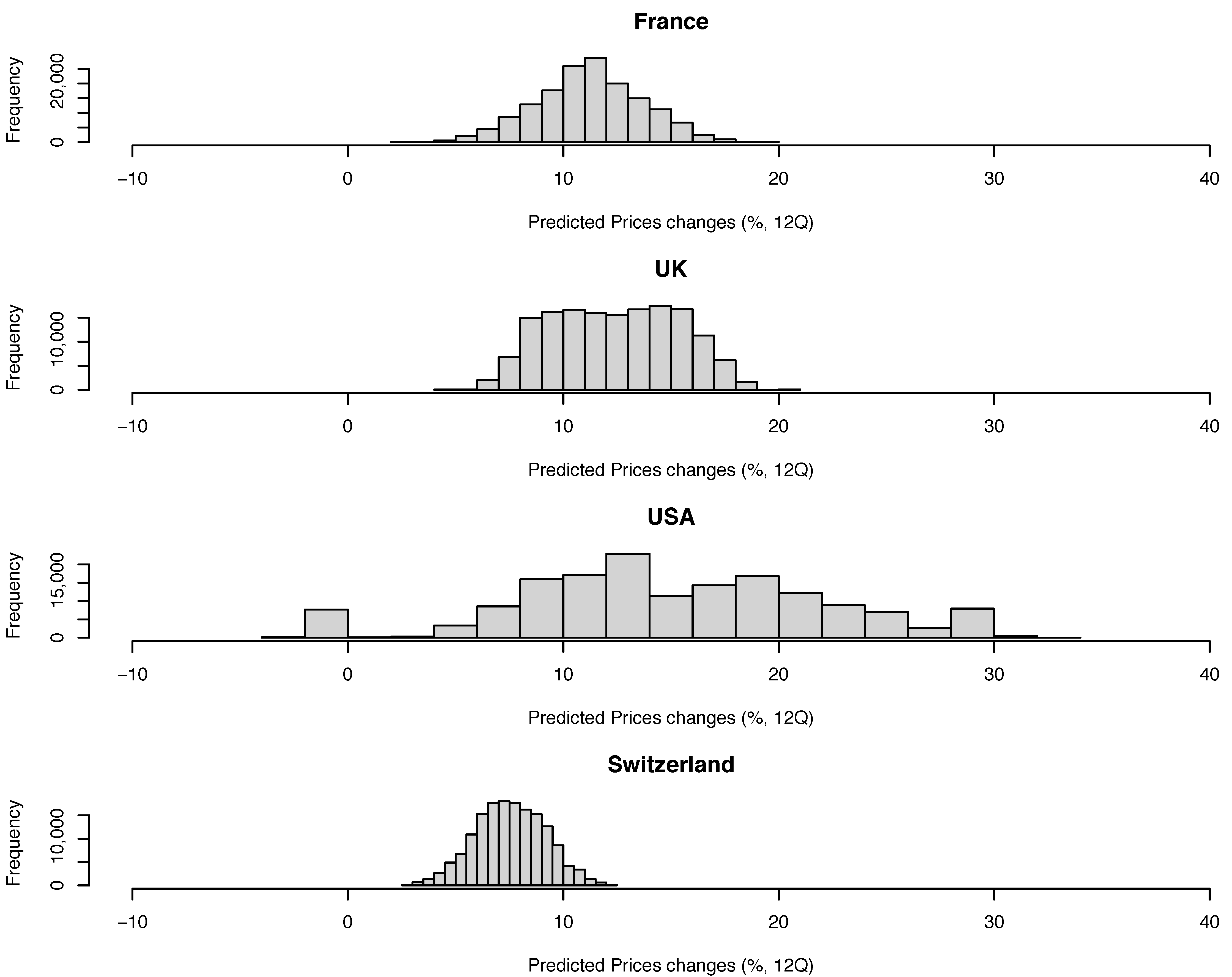
Figure 17.
Predicted price changes (over 12 quarters) for four countries. Those estimates need to be compared to the range of values of the RMS shown in the previous figure. Current values for France, UK, USA and Switzerland are 12.4%, 13.2%, 4.3%, 8.7%, respectively.
Figure 17.
Predicted price changes (over 12 quarters) for four countries. Those estimates need to be compared to the range of values of the RMS shown in the previous figure. Current values for France, UK, USA and Switzerland are 12.4%, 13.2%, 4.3%, 8.7%, respectively.
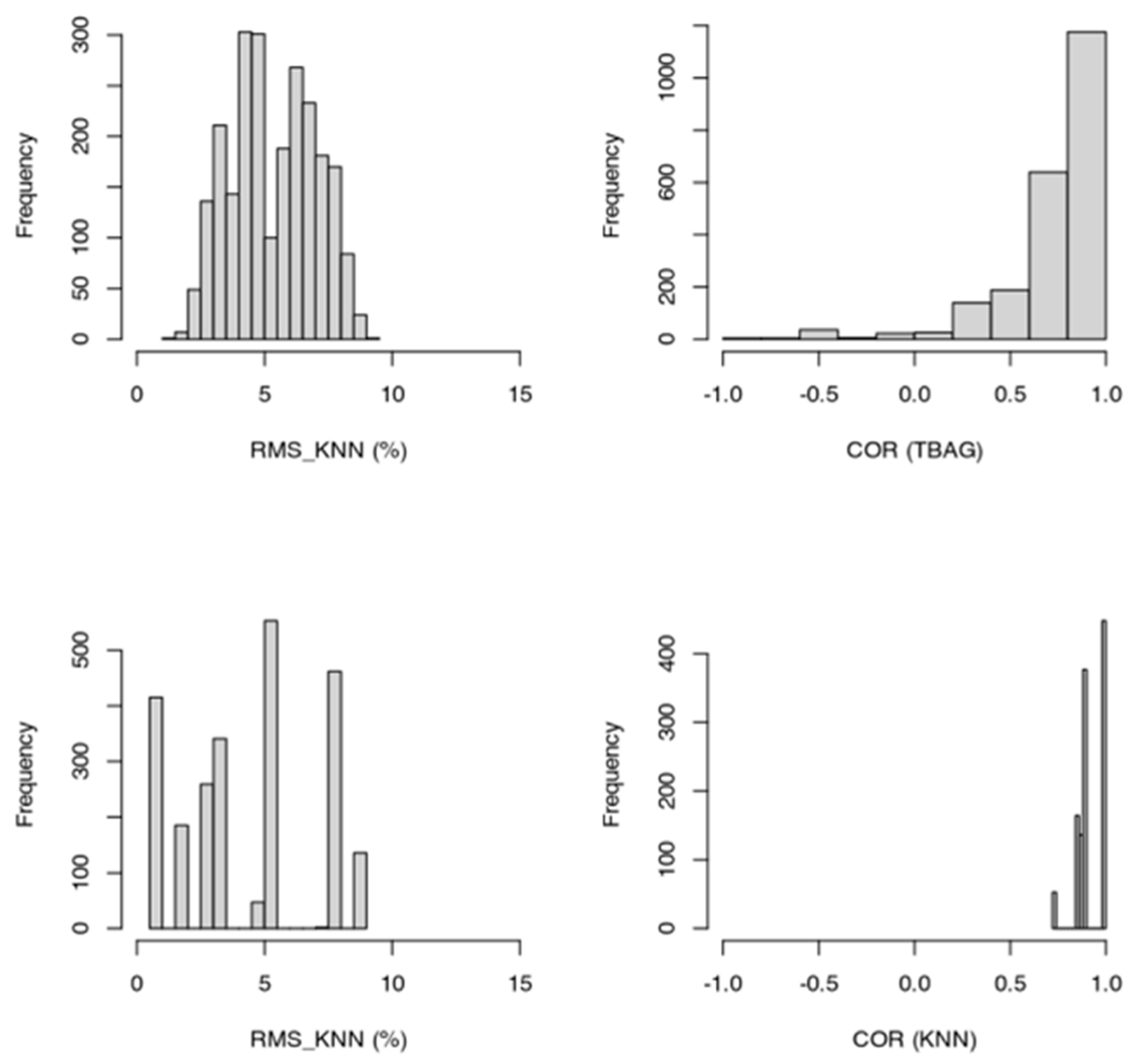
Figure 18.
Distributions of RMS and correlation parameters (COR) for the kNN and tree-bag strategies (data of the four countries are merged).
Figure 18.
Distributions of RMS and correlation parameters (COR) for the kNN and tree-bag strategies (data of the four countries are merged).
Table 1.
Training parameters used for all models in this study.
Table 1.
Training parameters used for all models in this study.
| Model Parameters | |
|---|
| tr control | method = “repeatedcv”, repeats = 3 |
| empty data | not allowed |
Table 2.
Characteristics of the data used for each model group. HPI rates are computed over 12 quarters
1.
Table 2.
Characteristics of the data used for each model group. HPI rates are computed over 12 quarters
1.
| | Model Name | GDP | CPI (Rates) | Treasury 10 y | Unemployment | Rent | Central Bank | ECB | HPI | Figure |
|---|
| 1 | 3-parameter | Y | Y | Y, rates | N | N | N | N | Nominal | Figure 4 |
| 2 | IR models | Y, rates | Y, rates | Y, rates | N | N | Y, US rates | N | Nominal | Figure 5
|
| 3 | Local Central bank | Y, rates | Y, rates | Y, rates | N | N | Y, local rates | N | Nominal | Figure 6
|
| 4 | ECB | Y, rates | Y, rates | Y, rates | N | N | N | Y, nominal | Nominal | Figure 7
|
| 5 | ECB/FED | Y, rates | Y, rates | Y, rates | N | N | Y, plus FED rates | Y | Nominal | Figure 8
|
| 6 | Rents | Y, rates | Y, rates | Y, rates | N | Y | N | N | Nominal | Figure 9
|
| 7 | 3-parameter 1 yr | Y, rates | Y, rates | Y, rates | N | N | N | N | Rates | Figure 10 |
| 8 | ECB 1 yr | Y, rates | Y, rates | Y, rates | N | N | N | Y | Rates | Figure 11
|
| 9 | Rent 1 yr | Y, rates | Y, rates | Y, rates | N | Y | N | N | Rates | Figure 12
|
| 10 | Permutations | Y, rates | Y, rates | Y, rates | N | N | N | N | Nominal | Figure 13
|
| 11 | LOCAL 1 yr | Y, rates | Y, rates | Y, rates | Y | N | N | N | Nominal | Figure 14
|
Table 3.
The first 20 most contributing variables selected by the kNN algorithm from the complete dataset of 49 parameters for model 1. Those parameters, in their original form (nominal values and percentages), are needed to explain apartment prices in Switzerland.
Table 3.
The first 20 most contributing variables selected by the kNN algorithm from the complete dataset of 49 parameters for model 1. Those parameters, in their original form (nominal values and percentages), are needed to explain apartment prices in Switzerland.
| | Parameter Name (SNB Denomination) | Category | Relative Importance |
|---|
| 1 | Compensation of employees paid to the rest of the world | Income | 100.00 |
| 2 | Type of goods - Goods - Durables | CPI | 99.55 |
| 3 | Type of goods - Services - Total | CPI | 99.49 |
| 4 | Compensation of employees | Income | 99.24 |
| 5 | Type of goods - Services - Private | CPI | 99.02 |
| 6 | Origin of goods - Domestic | CPI | 98.69 |
| 7 | Gross domestic product | Income | 97.09 |
| 8 | Gross national income GNI | Income | 96.95 |
| 9 | Subsidies | State | 96.78 |
| 10 | Consumption of fixed capital | Investment | 95.95 |
| 11 | Taxes on production and imports | State | 95.34 |
| 12 | Type of goods - Services - Public | Inflation | 91.33 |
| 13 | United Kingdom - GBP - GBP LIBOR - 3-month | Markets | 91.32 |
| 14 | Labour force | Demography | 88.95 |
| 15 | Compensation of employees received from the rest of the world | Income | 88.37 |
| 16 | Switzerland - CHF - Call money rate Tomorrow next - 1 day | Markets | 86.84 |
| 17 | CPI - Total index | Inflation | 84.31 |
| 18 | Net operating surplus | Production | 75.30 |
| 19 | Type of goods - Goods - Non-durables | Inflation | 73.91 |
| 20 | Property income paid to the rest of the world | Income | 72.37 |
Table 4.
List of parameters chosen for model 2. Here, as some parameters include some collinearity with prices (positive for Compensation of employees and GNI; negative for US LIBOR 3 m) the performance of this model should be considered with caution. However, this model presents the advantage of using raw data. This model also presents the advantage of linking some demographics data such as immigration numbers (more workers may lead to a decrease of salary levels).
| | Parameter Name
(SNB Denomination) | Category | Relative Importance |
|---|
| 1 | Compensation of employees | Income | 100 |
| 2 | GNI | Income | 96 |
| 3 | Inflation total index (%) | Inflation | 62 |
| 4 | US LIBOR 3m (%) | Rates | 24 |
| 5 | SNB Core inflation (%) | Rates | 0 |
Table 5.
Performance of the first two models based on Swiss National Bank dataset. The model (“lightdata”), which uses fewer input parameters but spans a more extended period, is more accurate (RMS, SD improve while COR and MAPE stay satisfactory). I consider both models are performing well (RMS < 15; MAPE < 0.2; COR > 0.90).
| Model | M_COR | S_COR | M_RMS | S_RMS | SD | M_MAE | M_MAPE | M_CHIp | M_CHIs |
|---|
| Model 1/49v | 0.994 | 0.001 | 3.307 | 0.201 | 3.320 | 2.649 | 0.020 | 0.157 | 0.213 |
| Model 2/“lightdata” | 0.974 | 0.001 | 0.464 | 0.009 | 0.466 | 0.373 | 0.110 | 0.095 | 0.702 |
Table 6.
Correlation coefficients of house price indices between countries for 10 countries. Values larger than 0.80 are highlighted in red. Four datasets (Italy, Finland, Japan, and Spain) correlate less with other price series. UK, Sweden, Australia, and the Netherlands show the strongest correlation with prices in the USA. Russia and Japan only publish yearly data for their Gross Domestic Product statistics. In the rest of the article, those two countries are excluded from the pool of countries modeled. Anti-correlations are indicated in green.
| | | Nobs | USA | FR | GER | SP | IT | FIN | SWE | AU | UK | CH | NL | RU | JP | HU | NO |
|---|
| 1 | USA | 196 | 1 | 0.89 | 0.91 | 0.75 | −0.01 | 0.79 | 0.94 | 0.96 | 0.98 | 0.82 | 0.95 | 0.84 | −0.32 | 0.93 | 0.99 |
| 2 | France | 174 | | 1 | 0.57 | 0.83 | 0.21 | 0.98 | 0.88 | 0.90 | 0.95 | 0.87 | 0.86 | 0.94 | −0.96 | 0.84 | 0.90 |
| 3 | Germany | 132 | | | 1 | 0.82 | 0.11 | 0.61 | 0.92 | 0.94 | 0.97 | 0.84 | 0.85 | 0.53 | −0.48 | 0.96 | 0.80 |
| 4 | Spain | 116 | | | | 1 | 0.67 | 0.22 | 0.64 | 0.66 | 0.78 | 0.54 | 0.83 | 0.57 | −0.88 | −0.13 | 0.62 |
| 5 | Italy | 116 | | | | | 1 | 0.53 | 0.20 | 0.17 | 0.01 | 0.28 | 0.19 | 0.94 | −0.30 | −0.61 | −0.19 |
| 6 | Finland | 136 | | | | | | 1 | 0.84 | 0.82 | 0.75 | 0.80 | 0.66 | 0.84 | −0.95 | 0.66 | 0.94 |
| 7 | Sweden | 124 | | | | | | | 1 | 0.99 | 0.97 | 0.95 | 0.87 | 0.84 | −0.86 | 0.93 | 0.99 |
| 8 | Australia | 195 | | | | | | | | 1 | 0.98 | 0.91 | 0.85 | 0.83 | −0.32 | 0.87 | 0.99 |
| 9 | UK | 195 | | | | | | | | | 1 | 0.86 | 0.92 | 0.83 | −0.27 | 0.90 | 0.97 |
| 10 | CH | 176 | | | | | | | | | | 1 | 0.74 | 0.83 | −0.53 | 0.76 | 0.90 |
| 11 | NL | 112 | | | | | | | | | | | 1 | 0.64 | −0.84 | 0.91 | 0.82 |
| 12 | Russia | 21 | | | | | | | | | | | | 1 | −0.92 | 0.61 | 0.86 |
| 13 | Japan | 46 | | | | | | | | | | | | | 1 | 0.17 | −0.52 |
| 14 | Hungary | 67 | | | | | | | | | | | | | | 1 | 0.85 |
| 15 | Norway | 184 | | | | | | | | | | | | | | | 1 |
Table 7.
Broad characteristics of the market. ARMS: Adjustable-Rate Mortgage.
Table 7.
Broad characteristics of the market. ARMS: Adjustable-Rate Mortgage.
| | Amortization | Fixed Rates? | Source |
|---|
| USA | Yes, continuous | Possible (ARM, 10%) | https://shorturl.at/g9bZ3, accessed on 6 January 2023. |
| France | Yes, continuous | Yes, variable 30% | https://shorturl.at/D4FOW, accessed on 6 January 2023. |
| UK | Yes | Possible, 26% | https://shorturl.at/FaNlm, accessed on 6 January 2023. |
| Switzerland | At least 35% after 10–15 yrs, otherwise discontinuous. | Yes, LIBOR for 10–15%,
ARM 5% | https://shorturl.at/bFb3b, accessed on 6 January 2023.
https://www.moneyland.ch/en/variable-rate-mortgages-comparison, accessed on 6 January 2023. |
Table 8.
Variable importance data for the models presented in this paper for Switzerland. The effect of the ECB dataset is visible in the improvement of the model performances.
Table 8.
Variable importance data for the models presented in this paper for Switzerland. The effect of the ECB dataset is visible in the improvement of the model performances.
| | Model Name | TR | CPI | GDP | Central Bank Rate | Asset | Additional Data, Imp. |
|---|
| 1 | 3-param | 100 | >10 | >10 | - | - | - |
| 2 | 3-param 1 yr | 100 | >10 | >10 | - | - | - |
| 3 | Central bank IR models (US rate) | 100 | >5 | 0 | 75 | - | - |
| 4 | Local Central bank IR models (LIR) | 100 | 93 | 0 | 27.9 | - | - |
| 5 | ECB | 90.9 | 13.4 | 0 | - | 100 | |
| 6 | ECB/FED | 92.9 | >5 | >5 | - | 100 | FED. Rate 24.9 |
| 7 | ECB 1 yr | 100 | 5 | 0 | - | 1.7 | - |
| 8 | LOCAL | - | | 100 | 22.5 | - | - | Unemployment, 0 |
| 9 | LOCAL 1 yr | - | | 100 | 43 | | | Unemployment, 0 |
| 10 | Rents | 100 | 0.8 | 0 | - | - | Rent index, 87.0 |
| 11 | Rents 1 yr | 78.4 | >1 | 0 | - | - | Rent index, 100 |
Table 9.
Same as
Table 8 for the tree-bag approach.
Table 9.
Same as
Table 8 for the tree-bag approach.
| | Model Name | Father | TR | CPI | GDP | Central Bank Rate | Asset | Additional Data, Imp. |
|---|
| 1 | 3-param | - | 100 | 13.4 | 0 | - | - | - |
| 2 | 3-param 1 yr | - | 100 | 1.3 | 0 | - | - | - |
| 3 | Central bank IR models (US rate) | 1 | 100 | 12.6 | 0 | 86.2 | - | - |
| 4 | Local Central bank IR models | 1 | 80.8 | 100 | 0 | 56.6 | - | - |
| 5 | ECB | 1 | 90.9 | 13.4 | 0 | - | 100 | |
| 6 | ECB/FED | 1, 4 | 76.8 | >5 | 0 | - | 100 | FED. rate > 5 |
| 7 | ECB 1 yr | 2 | 100 | 5 | 0 | - | 1.7 | - |
| 8 | LOCAL | - | | 100 | 0 | - | - | Unemployment, 22.8 |
| 9 | LOCAL 1 yr | | | 100 | 0 | | | 17.6 |
| 10 | Rents | | 77 | >10 | 0 | - | - | Rent index, 100 |
| 11 | Rents 1 yr | | 61.5 | >5 | 0 | - | - | Rent index, 100 |
Table 10.
Statistics of the data fit performance of the 3-parameters models (tree-bag strategy). HPI values are in nominal form. COR stands for Correlation, RMS for root mean square, MAE for mean absolute error, MAPE for mean absolute percentage error. CHIp and CHIs are the parameter and statistic of the Chi2.
| Countries | M_COR | S_COR | M_RMS | S_RMS | SD | M_MAE | M_MAPE | M_CHIp | M_CHIs |
|---|
| USA | 0.949 | 0.002 | 22.405 | 0.383 | 31.982 | 17.575 | 0.228 | 0.261 | 0.000 |
| France | 0.959 | 0.001 | 11.637 | 0.167 | 0.295 | 7.946 | 0.102 | 0.183 | 0.007 |
| Germany | 0.924 | 0.004 | 11.087 | 0.333 | 3.415 | 6.945 | 0.055 | 0.316 | 0.000 |
| Spain | 0.882 | 0.005 | 11.404 | 0.231 | 2.683 | 7.658 | 0.098 | 0.173 | 0.067 |
| Italy | 0.865 | 0.004 | 9.298 | 0.126 | 2.554 | 6.349 | 0.070 | 0.189 | 0.034 |
| Finland | 0.956 | 0.001 | 10.143 | 0.121 | 2.572 | 7.552 | 0.095 | 0.217 | 0.004 |
| Sweden | 0.956 | 0.003 | 19.687 | 0.661 | 20.861 | 15.148 | 0.125 | 0.166 | 0.066 |
| Australia | 0.956 | 0.002 | 21.044 | 0.433 | 14.522 | 15.866 | 0.247 | 0.215 | 0.000 |
| UK | 0.976 | 0.001 | 11.617 | 0.313 | 12.483 | 8.950 | 0.193 | 0.181 | 0.004 |
| Switzerland | 0.950 | 0.002 | 8.638 | 0.160 | 6.624 | 7.068 | 0.066 | 0.203 | 0.002 |
| Netherland | 0.865 | 0.011 | 16.400 | 0.514 | 17.635 | 12.710 | 0.123 | 0.160 | 0.131 |
| Norway | 0.965 | 0.001 | 18.465 | 0.339 | NA | 14.244 | 0.178 | 0.149 | 0.037 |
Table 11.
Statistics of the data fit performance of the IR models (tree-bagging strategy). COR stands for Correlation, RMS for root mean squared, MAE for mean absolute error, MAPE for mean absolute percentage error. CHIp and CHIs are the parameter and statistic of the Chi2.
Table 11.
Statistics of the data fit performance of the IR models (tree-bagging strategy). COR stands for Correlation, RMS for root mean squared, MAE for mean absolute error, MAPE for mean absolute percentage error. CHIp and CHIs are the parameter and statistic of the Chi2.
| Countries | M_COR | S_COR | M_RMS | S_RMS | SD | M_MAE | M_MAPE | M_CHIp | M_CHIs |
|---|
| USA | 0.963 | 0.002 | 18.871 | 0.443 | 18.999 | 14.092 | 0.204 | 0.262 | 0.000 |
| France | 0.960 | 0.001 | 11.550 | 0.183 | 3.310 | 7.964 | 0.105 | 0.186 | 0.006 |
| Germany | 0.917 | 0.008 | 11.457 | 0.456 | 8.660 | 7.123 | 0.055 | 0.353 | 0.000 |
| Spain | 0.890 | 0.005 | 11.144 | 0.240 | 3.178 | 7.255 | 0.094 | 0.135 | 0.255 |
| Italy | 0.893 | 0.005 | 8.431 | 0.155 | 3.264 | 5.405 | 0.061 | 0.198 | 0.025 |
| Finland | 0.954 | 0.001 | 10.373 | 0.131 | 3.170 | 7.729 | 0.097 | 0.212 | 0.005 |
| Sweden | 0.953 | 0.002 | 20.070 | 0.495 | 9.510 | 15.929 | 0.135 | 0.167 | 0.066 |
| Australia | 0.965 | 0.002 | 18.624 | 0.430 | 13.469 | 13.785 | 0.233 | 0.214 | 0.000 |
| UK | 0.968 | 0.001 | 13.066 | 0.210 | 7.663 | 10.131 | 0.240 | 0.216 | 0.000 |
| Switzerland | 0.961 | 0.001 | 7.472 | 0.126 | 2.100 | 5.972 | 0.057 | 0.182 | 0.007 |
| Netherland | 0.879 | 0.008 | 14.983 | 0.409 | 6.807 | 11.102 | 0.110 | 0.166 | 0.112 |
| Norway | 0.994 | 0.000 | 7.399 | 0.269 | NA | 5.752 | 0.084 | 0.134 | 0.081 |
Table 12.
Statistics of the data fit performance of the LIR (local interest rates) models (tree-bagging strategy). COR stands for Correlation, RMS for root mean squared, MAE for mean absolute error, MAPE for mean absolute percentage error. CHIp and CHIs are the parameter and statistic of the Chi2. Models with RMS < 20 and MAPE less than 20% are considered as performing.
| Countries | M_COR | S_COR | M_RMS | S_RMS | SD | M_MAE | M_MAPE | M_CHIp | M_CHIs |
|---|
| USA | 0.961 | 0.002 | 19.323 | 0.400 | 18.720 | 14.538 | 0.214 | 0.263 | 0.000 |
| France | 0.897 | 0.004 | 12.552 | 0.191 | 6.631 | 9.746 | 0.098 | 0.193 | 0.061 |
| Germany | 0.864 | 0.011 | 15.170 | 0.558 | 5.149 | 8.765 | 0.065 | 0.261 | 0.003 |
| Spain | 0.850 | 0.010 | 10.154 | 0.234 | 3.019 | 6.801 | 0.083 | 0.163 | 0.161 |
| Italy | 0.857 | 0.008 | 7.797 | 0.150 | 2.474 | 5.210 | 0.058 | 0.229 | 0.017 |
| Finland | 0.923 | 0.003 | 9.365 | 0.169 | 8.135 | 6.541 | 0.067 | 0.167 | 0.139 |
| Sweden | 0.900 | 0.006 | 24.037 | 0.733 | 53.721 | 16.982 | 0.125 | 0.165 | 0.254 |
| Australia | 0.965 | 0.001 | 17.924 | 0.367 | 32.903 | 12.277 | 0.212 | 0.214 | 0.001 |
| UK | 0.963 | 0.002 | 13.596 | 0.260 | 3.191 | 10.558 | 0.253 | 0.226 | 0.001 |
| Switzerland | 0.975 | 0.003 | 5.885 | 0.304 | 16.130 | 4.332 | 0.041 | 0.163 | 0.031 |
| Netherland | 0.873 | 0.014 | 13.497 | 0.464 | 6.959 | 9.563 | 0.086 | 0.212 | 0.026 |
| Norway | 0.964 | 0.002 | 16.851 | 0.443 | NA | 12.070 | 0.123 | 0.264 | 0.001 |
Table 13.
Statistics of the data fit performance of the ECB models (tree-bagging strategy). COR stands for Correlation, RMS for root mean squared, MAE for mean absolute error, MAPE for mean absolute percentage error. CHIp and CHIs are the parameter and statistic of the Chi2.
Table 13.
Statistics of the data fit performance of the ECB models (tree-bagging strategy). COR stands for Correlation, RMS for root mean squared, MAE for mean absolute error, MAPE for mean absolute percentage error. CHIp and CHIs are the parameter and statistic of the Chi2.
| Countries | M_COR | S_COR | M_RMS | S_RMS | SD | M_MAE | M_MAPE | M_CHIp | M_CHIs |
|---|
| USA | 0.983 | 0.001 | 12.937 | 0.232 | 3.121 | 10.908 | 0.202 | 0.265 | 0.001 |
| France | 0.993 | 0.001 | 5.019 | 0.176 | 0.829 | 3.787 | 0.059 | 0.159 | 0.030 |
| Germany | 0.985 | 0.001 | 4.982 | 0.201 | 3.129 | 3.739 | 0.031 | 0.400 | 0.001 |
| Spain | 0.980 | 0.002 | 4.806 | 0.194 | 1.286 | 3.582 | 0.047 | 0.181 | 0.045 |
| Italy | 0.978 | 0.002 | 3.905 | 0.136 | 0.198 | 3.151 | 0.036 | 0.243 | 0.002 |
| Finland | 0.985 | 0.001 | 5.923 | 0.136 | 2.450 | 4.831 | 0.064 | 0.204 | 0.008 |
| Sweden | 0.992 | 0.000 | 8.463 | 0.211 | 3.544 | 6.431 | 0.055 | 0.151 | 0.122 |
| Australia | 0.988 | 0.001 | 11.212 | 0.390 | 7.948 | 9.038 | 0.199 | 0.212 | 0.000 |
| UK | 0.984 | 0.001 | 9.399 | 0.217 | 1.096 | 7.665 | 0.204 | 0.191 | 0.002 |
| Switzerland | 0.976 | 0.001 | 5.995 | 0.100 | 0.147 | 4.861 | 0.049 | 0.193 | 0.003 |
| Netherland | 0.981 | 0.002 | 6.220 | 0.348 | 4.405 | 5.218 | 0.054 | 0.207 | 0.018 |
| Norway | 0.990 | 0.001 | 9.631 | 0.310 | NA | 7.755 | 0.133 | 0.200 | 0.003 |
Table 14.
Statistics of the data fit performance of the ECB/FED models (tree-bagging strategy). COR stands for Correlation, RMS for root mean squared, MAE for mean absolute error, MAPE for mean absolute percentage error. CHIp and CHIs are the parameter and statistic of the Chi2.
Table 14.
Statistics of the data fit performance of the ECB/FED models (tree-bagging strategy). COR stands for Correlation, RMS for root mean squared, MAE for mean absolute error, MAPE for mean absolute percentage error. CHIp and CHIs are the parameter and statistic of the Chi2.
| Countries | M_COR | S_COR | M_RMS | S_RMS | SD | M_MAE | M_MAPE | M_CHIp | M_CHIs |
|---|
| USA | 0.985 | 0.001 | 12.428 | 0.220 | 1.929 | 10.599 | 0.196 | 0.262 | 0.001 |
| France | 0.993 | 0.001 | 5.009 | 0.193 | 0.828 | 3.758 | 0.060 | 0.165 | 0.025 |
| Germany | 0.980 | 0.002 | 5.642 | 0.230 | 3.827 | 3.979 | 0.032 | 0.381 | 0.001 |
| Spain | 0.983 | 0.002 | 4.435 | 0.187 | 1.146 | 3.404 | 0.044 | 0.182 | 0.044 |
| Italy | 0.974 | 0.002 | 4.216 | 0.130 | 0.434 | 3.500 | 0.040 | 0.246 | 0.002 |
| Finland | 0.987 | 0.001 | 5.468 | 0.116 | 2.450 | 4.490 | 0.060 | 0.232 | 0.002 |
| Sweden | 0.993 | 0.000 | 7.707 | 0.186 | 3.121 | 5.585 | 0.050 | 0.154 | 0.110 |
| Australia | 0.989 | 0.001 | 10.814 | 0.372 | 8.358 | 8.440 | 0.186 | 0.204 | 0.001 |
| UK | 0.984 | 0.001 | 9.234 | 0.214 | 1.346 | 7.465 | 0.208 | 0.196 | 0.002 |
| Switzerland | 0.975 | 0.001 | 6.095 | 0.099 | 0.301 | 5.011 | 0.050 | 0.198 | 0.002 |
| Netherland | 0.980 | 0.003 | 6.371 | 0.383 | 2.271 | 5.420 | 0.056 | 0.203 | 0.023 |
| Norway | 0.995 | 0.000 | 7.000 | 0.291 | NA | 5.523 | 0.089 | 0.141 | 0.058 |
Table 15.
Statistics of the data fit performance of the 3-parameters-1 yr models (tree-bagging strategy). COR stands for Correlation, RMS for root mean squared, MAE for mean absolute error, MAPE for mean absolute percentage error. CHIp and CHIs are the parameter and statistic of the Chi2.
Table 15.
Statistics of the data fit performance of the 3-parameters-1 yr models (tree-bagging strategy). COR stands for Correlation, RMS for root mean squared, MAE for mean absolute error, MAPE for mean absolute percentage error. CHIp and CHIs are the parameter and statistic of the Chi2.
| Countries | M_COR | S_COR | M_RMS | S_RMS | SD | M_MAE | M_MAPE | M_CHIp | M_CHIs |
|---|
| USA | 0.812 | 0.008 | 7.605 | 0.105 | 4.338 | 5.646 | 1.099 | 0.191 | 0.003 |
| France | 0.838 | 0.005 | 6.019 | 0.066 | 2.383 | 4.712 | 0.992 | 0.240 | 0.000 |
| Germany | 0.872 | 0.004 | 3.840 | 0.055 | 4.925 | 2.809 | 2.197 | 0.240 | 0.001 |
| Spain | 0.873 | 0.005 | 8.328 | 0.135 | 2.025 | 6.427 | 1.233 | 0.142 | 0.193 |
| Italy | 0.954 | 0.001 | 10.382 | 0.136 | 2.450 | 7.648 | 0.096 | 0.217 | 0.004 |
| Finland | 0.848 | 0.006 | 4.522 | 0.081 | 4.528 | 3.717 | 0.360 | 0.204 | 0.012 |
| Sweden | 0.808 | 0.006 | 6.471 | 0.071 | 1.446 | 5.200 | 0.346 | 0.212 | 0.000 |
| Australia | 0.891 | 0.004 | 6.736 | 0.110 | 1.070 | 5.204 | 1.515 | 0.147 | 0.042 |
| UK | 0.887 | 0.004 | 4.483 | 0.066 | 1.508 | 3.328 | 0.565 | 0.280 | 0.000 |
| Switzerland | 0.777 | 0.013 | 9.610 | 0.125 | 1.429 | 8.201 | 4.069 | 0.255 | 0.002 |
| Netherland | 0.707 | 0.012 | 23.067 | 0.290 | 3.350 | 16.908 | 0.838 | 0.571 | 0.001 |
| Norway | NA | 0.000 | NA | 0.000 | NA | 14.244 | 0.178 | 0.149 | 0.037 |
Table 16.
Statistics of the data fit performance of the ECB 1 yr models (tree-bagging strategy). COR stands for Correlation, RMS for root mean squared, MAE for mean absolute error, MAPE for mean absolute percentage error. CHIp and CHIs are the parameter and statistic of the Chi2.
Table 16.
Statistics of the data fit performance of the ECB 1 yr models (tree-bagging strategy). COR stands for Correlation, RMS for root mean squared, MAE for mean absolute error, MAPE for mean absolute percentage error. CHIp and CHIs are the parameter and statistic of the Chi2.
| Countries | M_COR | S_COR | M_RMS | S_RMS | SD | M_MAE | M_MAPE | M_CHIp | M_CHIs |
|---|
| USA | 0.850 | 0.007 | 6.680 | 0.121 | 4.901 | 4.828 | 1.230 | 0.159 | 0.023 |
| France | 0.923 | 0.003 | 4.255 | 0.073 | 1.416 | 3.300 | 1.073 | 0.151 | 0.051 |
| Germany | 0.933 | 0.003 | 2.878 | 0.052 | 4.986 | 2.180 | 4.607 | 0.262 | 0.001 |
| Spain | 0.956 | 0.002 | 5.200 | 0.112 | 1.285 | 3.930 | 0.303 | 0.142 | 0.248 |
| Italy | 0.958 | 0.004 | 3.647 | 0.166 | 1.764 | 2.758 | 2.252 | 0.143 | 0.250 |
| Finland | 0.774 | 0.010 | 9.773 | 0.180 | 2.622 | 5.984 | 1.067 | 0.209 | 0.012 |
| Sweden | 0.866 | 0.009 | 3.824 | 0.099 | 3.415 | 3.166 | 0.233 | 0.214 | 0.019 |
| Australia | 0.895 | 0.005 | 4.723 | 0.091 | 1.657 | 3.918 | 0.243 | 0.191 | 0.003 |
| UK | 0.893 | 0.004 | 6.648 | 0.085 | 1.101 | 5.177 | 0.595 | 0.156 | 0.027 |
| Switzerland | 0.914 | 0.003 | 3.935 | 0.059 | 1.401 | 2.742 | 0.417 | 0.212 | 0.002 |
| Netherland | 0.958 | 0.003 | 4.203 | 0.146 | 1.388 | 2.888 | 0.487 | 0.115 | 0.532 |
| Norway | 0.991 | 0.001 | 9.400 | 0.309 | NA | 7.492 | 0.129 | 0.200 | 0.003 |
Table 20.
Range of MEF values used to compute the predicted values (160,000 models). For each parameter, 20 values were tested over each range.
Table 20.
Range of MEF values used to compute the predicted values (160,000 models). For each parameter, 20 values were tested over each range.
| N | GDP (%) | Inflation (CPI) | ECB Asset Size (M EUR) | Treasury Rates (%) |
|---|
| 160,000 | −2 to 2% | −2 to 2% | 6.5 × 10⁶ ± 1 × 10⁶ | 0 to 4% |


