Article

Exploring the Nature and Dynamics of Monetary–Fiscal Policy Interactions in South Africa

by
Amanda Mavundla
*,
Simiso Msomi
and
Malibongwe Cyprian Nyati
School of Accounting, Economics and Finance, College of Law and Management Studies, University of KwaZulu Natal, Durban 3629, South Africa
*
Author to whom correspondence should be addressed.
Risks 2025, 13(10), 185; https://doi.org/10.3390/risks13100185
Submission received: 10 July 2025 / Revised: 4 September 2025 / Accepted: 4 September 2025 / Published: 26 September 2025

Abstract

Understanding the nature of monetary and fiscal policy interactions has gained more importance over the years, especially within the context of the global financial crisis and the recent COVID-19 pandemic. This study uses a Time-Varying Parameter Vector Autoregressive (TVP-VAR) model and a Markov Switching Dynamic Regression (MSDR) framework to explore the dynamics of monetary–fiscal policy interactions in South Africa. The analysis employs time series data from 1994 to 2023 and tests the dynamic response of key macroeconomic variables to positive monetary and fiscal policy shocks. Furthermore, the MSDR framework is utilised to analyse how policy behaviour evolves during regime change. The TVP-VAR results show that fiscal expansions led to a positive response in GDP over time, a stable interest rate reaction post-COVID-19, and a consistently negative CPI response, contradicting conventional theory. The MSDR analysis reveals a dominant regime where monetary policy is active and fiscal policy is passive, with a positive interaction between interest rates and government spending, likely reflecting South Africa’s high debt environment. These findings underscore the importance of understanding policy interactions’ landscape to inform policy decisions better and minimise sub-optimal policy outcomes.

1. Introduction

An increasing mutual consensus has favoured separating the monetary and fiscal policy powers in pursuing the primary macroeconomic objectives of stabilising the economy and sustaining non-inflationary economic growth (Oboh 2017). Attaining macroeconomic stability makes a country less susceptible to external shocks and helps maintain a steady course toward long-term, sustainable economic growth (Nasrullah et al. 2023). The main tools policy authorities use to attain macroeconomic stability and long-term economic growth are monetary policy (MP) and fiscal policy (FP). Several policy instruments have been developed to assist policy authorities in achieving their objectives (Du Plessis et al. 2007). There has been general acceptance of how both policies play a vital role in economic activities. However, different arguments exist on the preferred policy to achieve macroeconomic stability (Šehović 2013). Before the onset of the 2008 Global Financial Crisis (GFC), the dominant view among economists and policymakers was that MP was best suited to macroeconomic volatility, while FP was primarily viewed as a secondary instrument, constrained by political lags and best reserved for long-term structural objectives (Hammoudeh et al. 2015). FP’s focus is mainly on public finances and ensuring that long-term economic growth is achieved. The recent global economic events, such as the GFC, the increasing development of Monetary unions, and the recent COVID-19 pandemic, have seen more counteractive behaviour between these policies (Chibi et al. 2019). Additionally, there is an inefficiency in using one policy to deter and manage economic shocks.
The increasing development of monetary unions brings about a new macroeconomic regime. With the centralised control of MP within the union, the FP need not be counteractive regarding its objectives (Cevik et al. 2014). Maintaining stable prices is the primary responsibility of the central bank, and second in line is to support general economic objectives (Claeys 2004). The monetary union pact rules require automatic stabilisers around fiscal positions that are structurally sound. Additionally, Canzoneri et al. (2003) highlight that in a monetary union, MP and FP’s effectiveness and transmission pathways can evolve in response to changing economic conditions. The success of FP will depend significantly on the interdependent interactions between the various budgetary authorities. Additionally, the 2008 GFC destabilised economies and impeded economic growth (da Silva and Vieira 2017). This made it impossible for a single policy to stabilise and recover from the effects of the GFC. For example, many developed countries faced a “zero lower bound” after the GFC. Thus, there is a need to coordinate both policies to deal with macroeconomic shocks. The role of MP lies with the monetary authorities, while the role and responsibility of FP are entirely up to elected public authorities (Canzoneri et al. 2003). These economic policies may entail different objectives and employ different methods to achieve macroeconomic stability (Büyükbaşaran et al. 2020).
Policymakers and economists have investigated which economic policy is more effective. However, the effectiveness of both policies may differ according to the present economic conditions and characteristics (Tuncer and Akıncı 2018). The effectiveness of both these policies has become more apparent with the development of the monetary unions and the recent global financial crisis. Both these events stressed the importance of coordinating these policies. Afonso and Sousa (2020) argue that fiscal actions may compromise the success of MP by affecting short-run demand dynamics and diminishing confidence in its effectiveness. The effects of FP on MP also include long-term alterations of the economic conditions through growth and inflation (Afonso and Gonçalves 2020). According to Arby and Hanif (2010), FP focuses on attaining economic growth, and employment can sometimes be at the detriment of inflation. While the pursuit of FP to achieve macroeconomic objectives can be counteractive to MP, the same is true for the effects of MP on FP.
From a South African (SA) setting, there is a level of independence in the execution and interaction of MP and FP to ensure macroeconomic stability. The South African Reserve Bank (SARB) employs MP to regulate inflation and interest rates. At the same time, the National Treasury uses FP to regulate taxes and government expenditures (Du Plessis et al. 2007). The two policies can sometimes complement one another, as the SARB interest rates influence the cost of borrowing for the government’s fiscal interventions (Leshoro 2020). Moreover, they can also be counterproductive to one another in achieving set policy objectives. The SARB’s inflation-targeting instrument can often be used against the government’s planned spending priorities. The counteractive actions of both these policies have seen an increase in inflation rates to almost 9% over the years. This has been paralleled by a steady increase in the nation’s debt burden (IMF 2023).
SA’s economic landscape, marked by structural and policy challenges, offers a critical case for studying MP-FP interactions. Persistent fiscal deficits, rising debt-to-GDP ratios, and revenue constraints have weakened countercyclical fiscal policy effectiveness (National Treasury of South Africa 2023). While the SARB follows inflation targeting, fiscal pressures risk undermining monetary policy credibility (SARB 2023). As a small open economy, South Africa also faces external shocks, including commodity price volatility and exchange rate instability (Ocran 2019). These challenges highlight the need to analyse MP-FP dynamics over time.
Considering those mentioned earlier, the primary objective of this study is to examine the dynamic interaction between MP and FP in SA, focusing on time-varying effects and regime shifts. To achieve this, the paper will first analyse FP’s time-varying responses to MP shocks, followed by an analysis of time-varying responses of MP to FP shocks and, lastly, exploring the interactions of MP and FP under varying economic regimes. Using a Time-Varying Parameter VAR (TVP-VAR) and a Markov Switching Dynamic Regression (MSR) framework, the analysis captures gradual and sudden shifts in policy dynamics, offering new insights into macroeconomic policy behaviour in different environments. Moreover, the paper will provide critical insights into the dynamic policy mix in SA, given its challenges with high public debt, persistent fiscal deficits and an inflation-growth trade-off economic landscape.
The organisation of the study is as follows: in Section 2, a review of the relevant literature regarding the topic is discussed. Section 3 discusses an analysis of the data and the methodology adopted. In Section 4, the data and results are presented and discussed. Finally, Section 5 concludes and makes recommendations.

2. Literature Review

Understanding the interactions of MP and FP has become increasingly crucial over the years, especially with regard to macroeconomic stability (Blanchard 2019). The importance of understanding these interactions has deepened given the presence of persistent fiscal pressures and increasing exposure to external shocks. The interaction of these policies influences key macroeconomic indicators such as interest rates, inflation, debt levels and ultimately economic growth. Existing literature offers three dominant perspectives on MP and FP interactions: The Fiscal Theory of Price Level (FTPL), strategic policy framed by game theory, and time-varying regime switching approaches.
The Fiscal Theory of the Price Level (FTPL), first introduced by Leeper (1991) and further developed by Sims (1994), Woodford (1995), and Cochrane (2001, 2021), challenges the traditional monetarist view that central banks alone determine the price level. The FTPL posits that fiscal factors such as budget constraints, public debt levels, and debt management are pivotal in price-level determination. Under this framework, fiscal policy (FP) and monetary policy (MP) are inherently interlinked: changes in interest rates not only influence aggregate demand and output but may also exacerbate debt sustainability concerns and heighten inflationary pressures in highly indebted economies. Moreover, inflation is shaped by conventional demand-pull mechanisms and by the FTPL’s distinct debt-revaluation channels (Cochrane 2021). Empirical evidence supports this perspective. Maitra and Hossain (2025), using a VAR model for India from 1985 to 2019, find that fiscal deficits tend to elevate the price level, whereas government spending can help stabilise its trajectory. Similarly, Barro and Bianchi (2023) apply the FTPL framework to OECD countries and show that weak fiscal discipline significantly contributes to higher inflation rates, reinforcing the theory’s relevance. In South Africa, Sangweni and Ngalawa (2023) employ a New Keynesian dynamic stochastic general equilibrium (NK-DSGE) model with financial frictions to examine inflation–debt dynamics. Their results corroborate that inadequate fiscal discipline undermines the South African Reserve Bank’s ability to maintain price stability, underscoring the critical role of fiscal credibility in monetary policy effectiveness.
While the FTPL frames policy interaction challenges primarily through the lens of fiscal dominance, the game-theoretic approach emphasises the strategic nature of policy decisions. This perspective conceptualises MP and FP interactions as a strategic game between policy authorities whose objectives may diverge or conflict (Heijmans 2023). Pioneering this framework, Dixit and Lambertini (2003) argue that MP–FP coordination can be effectively analysed using game theory, which examines how rational players make interdependent decisions to maximise their respective objectives, considering the likely responses of others (Zhang 2024). Within this approach, through their impact on borrowing costs and aggregate demand, interest rate adjustments influence both price stability and economic output (Aruoba and Drechsel 2024). Conversely, government spending decisions directly affect aggregate demand and GDP growth (Auerbach et al. 2021). Strategic misalignment in the dynamic interaction of MP-FP can result in increased inflationary pressures when a fiscal expansion coincides with accommodative MP and output contraction in the case of a simultaneous MP-FP tightening (Hooley et al. 2021). Empirically, Bassetto and Sargent (2020) employ a game-theoretic framework to analyse strategic MP-FP interactions; their findings suggest that the risk of fiscal dominance, particularly loss of FP credibility, reduces the central bank’s ability to control inflationary pressures. Chibi et al. (2024) further support these findings by employing dynamic stochastic game theory to model policy interaction in emerging economies. That fiscal austerity often follows monetary tightening due to credibility concerns. Additionally, Zhang (2024) employs Nash equilibrium game theory to analyse MP-FP interactions and finds that coordination between policies minimises welfare loss effectively and is crucial for economic stability.
A third and increasingly influential strand of research emphasises the dynamic and evolving nature of policy interactions. The time-varying regime theory in the context of policy interactions refers to the notion that the dynamics and coordination of MP and FP can change over time through the influence of structural, political, and economic factors (Bianchi and Melosi 2017). Studies employing structural vector autoregressive (SVAR), time-varying parameter (VAR) and dynamic stochastic general equilibrium (DSGE) models have indicated that the interaction of MP and FP influences key macroeconomic variables such as interest rates, government spending decisions, price stability and ultimately economic growth (Ascari et al. 2020). For instance, Jordà et al. (2023) investigate policy interaction; they analyse data from 17 OECD countries from 1860 to 2020. Findings indicate that a fiscal expansion increased interest rates, especially for countries with higher debt levels. While Corsetti et al. (2019), in an investigation of fiscal expansion on price stability for the Eurozone, find that a fiscal expansion led to increased inflationary pressures when MP is accommodative. Where monetary expansion effects are concerned, Reis (2023) analyses the effect of monetary expansion on debt sustainability and finds that quantitative easing (QE) eases debt servicing costs and enables higher debt-to-GDP ratios without causing fiscal stress. On the contrary, Shvets (2023) argue that prolonged monetary expansions can increase fiscal dominance risk. Additionally, Auerbach et al. (2021) employ a TVP-VAR to analyse the effects of MP on fiscal multipliers. Findings suggest that when MP is accommodative, fiscal multipliers increase.
In SA, empirical studies examining policy interactions remain limited. Buthelezi (2023) employs a Markov-Switching Dynamic Regression (MSDR) model to investigate MP and FP dynamics, finding that MP generally supports FP indicators. Majenge et al. (2024) adopt an Autoregressive Distributed Lag (ARDL) cointegration framework and Granger causality tests on data from 1980 to 2022, showing a long-term relationship between government spending, debt, and revenue. While these studies offer important insights, their methods assume discrete regime changes or constant long-run relationships. Such assumptions may be restrictive given SA’s substantial structural and institutional shifts since the 1980s. Approaches incorporating time-varying parameters would better capture policy interactions’ gradual and evolving nature, offering a more refined understanding of how these relationships adapt across macroeconomic environments.

3. Materials and Methods

To achieve the objectives of analysing dynamic MP and FP interactions in SA, this study employs the TVP-VAR and MSDR frameworks. These advanced econometric techniques are particularly suited for South Africa due to the economy’s structural shifts, policy regime changes, and exposure to external shocks. The advantages of the TVP-VAR lie in its ability to capture time-varying policy effects where a traditional VAR assumes constant parameters, which may be limiting to SA’s economic landscape, characterised by evolving policy transmission mechanisms.
Additionally, the TVP-VAR allows for a better analysis of how policy interactions evolve. At the same time, the use of the MSDR will assist in identifying distinct economic regimes (e.g., high-inflation vs. recessionary periods) in South Africa, where MP and FP interactions may shift abruptly due to policy changes. This paper will provide a comprehensive insight into MP and FP interactions in SA by employing these two methods.

3.1. Data and Variables

The study uses secondary data to achieve the set objectives. The data is extracted from the SARB database. This study utilises quarterly time-series data spanning 1994Q1 to 2023Q4, capturing SA’s complete post-apartheid economic history. The analysis incorporates five key macroeconomic variables: consumer price index (CPI) for inflation, real GDP for economic activity, government debt-to-GDP ratio (DEBT) for fiscal sustainability, the central bank policy rate (IR) as the MP indicator and government expenditure-to-GDP (GOV_2) as the FP indicator.

3.2. TVP-VAR Model

Researchers have extensively relied on conventional VAR models to analyse how MP and FP influence macroeconomic variables over time (see Mishra et al. 2012). The basic VAR model was initially developed by Sims (1980) and has been developed into different extended forms. Primiceri (2005) and Nakajima (2011) have extended and improved the model framework by incorporating time-varying parameters. Before a TVP-VAR model is made, the VAR must be specified in its basic form.
A y t = F 1 y t 1 + + F s y t s + u t   t = s + 1 , , n
In the above Equation (1) y t represents a k × 1 vector, which consists of observed variables; t represents the time ( t = s + 1 , , n ) ; s presents lag times; and A ,   F 1 F s represents k   × k coefficient matrices. The disturbance u t denotes a k × 1 structural shock in the economy, which follows u t ~ N ( 0 , ) , where
= σ 1 0 0 0 0 0 0 σ k
where σ denotes the standard deviation. With the assumption that structural shocks follow a recursive identification pattern, A takes a lower triangular matrix form as;
A = 1 0 0 a 21 0 a k 1 a k , k 1 1
The structural VAR from Equation (3) is transformed to a reduced form VAR model as follows:
y t = B 1 y t 1 + + B s y t s + A 1 ε t ,   ε t ~ N 0 , I k
B i = A 1 F i ,   i = 1 , , s
The elements in the rows of B i are stacked to form vector β k 2 s   × 1 , defining X t = I k ( y t 1 , , y t s ) , where the Kronecker product is denoted as ⊗. Thus, the model is further formulated as follows;
y t = X t β t + A t 1 ε t
Following the works of Primiceri (2005) and Nakajima (2011), the parameters ( β , A , ) in Equation (6) are allowed to be time-varying, and the TVP-VAR model with stochastic volatility can be written as follows:
y t = X t β t + A t 1 ε t ,   t = s + 1 , , n
Following Nakajima (2011), the lower-triangular elements in A t are converted to the forms a t = ( a 21 , a 31 , a 32 , a 41 , , a k , k 1 ) and h t = h 1 , t , , h k t h j , t = l o g σ j t 2 , for j = 1 , , k , t = s + 1 , , n to reduce the parameters that need to be estimated, and the parameters in Equation (7) assume a random walk process as follows:
β t + 1 = β t + u β t ,   α t + 1 = α t + u α t , h t + 1 = h t + u h t
ε t u β t u α t u h t ~ N 0 I 0 0 0 0 β 0 0 0 0 α 0 0 0 0 h
The initial states for the time-varying parameters are assumed to be given by β s + 1 ~ N ( u β 0 , β 0 ) , α s + 1 ~ N ( u α 0 , α 0 ) ,   h s + 1 ~ N ( u h 0 , h 0 ) . In the above matrix, there is no correlation among the time-varying parameters. Hence, the covariance matrices β , α and h are assumed to be diagonal (Nakajima 2011).
The TVP-VAR model estimation involves the computation and estimation of several parameters. The model estimation is also tricky due to the stochastic volatility and an intractable likelihood function. To avoid this challenge, the TVP-VAR is estimated based on Bayesian inference and the Markov Chain Monte Carlo (MCMC) approaches. Primiceri (2005), Nakajima (2011), and Banerjee and Malik (2012) argue that the Bayesian inference framework allows the original estimation challenge to be split up into smaller estimations to deal with the issue of high-dimensional parameters more efficiently. With the MCMC approach, the joint posterior distributions of the parameters are assessed in advance under specific priors. Additionally, the MCMC approach deals with recursive sampling from lower-dimensional objects and assists with parameter explosions (Nakajima 2011).
The priors used are derived from the work of Nakajima (2011), being β ~ I W 25 , 0.01 I ,   α i 2 ~ G a m m a 4 , 0.02 and h i 2 ~ G a m m a 4 , 0.02 . I W represents the inverted Wishart distribution, α i 2 and h i 2 denote the i = t h diagonal elements of the matrices.

3.3. The MSDR Model

The MSDR model was initially developed by Quandt (1972) and Goldfeld and Quandt (1973). This model is applied to time series that are thought to shift between a limited number of hidden regimes, enabling the behaviour of the process to vary across different states. The transitions occur according to a Markov process. The time of transition from one state to another and the duration between state changes is random. Considering a series with an evolution of y t , where t = 1,2 , ,   T , is characterised by two states, as is specified below:
State   1 :   y t = μ 1 + ε t
State   2 :   y t = μ 2 + ε t
where μ 1 and μ 2 represent the intercept terms in state 1 and state 2, respectively. Here, ε t represents the white noise error term with a variance σ 2 . The two states model shifts in its intercept term (Hamilton 1989; Hamilton 1990). If the timing of the switches is known, the model above can be expressed as;
y t = s t μ 1 + 1 s t μ 2 + ε t
where s t is 1 if the process is in state 1 and 0 if it is not. MSDR models are designed to capture swift transitions between regimes, making them well-suited for modelling data at monthly or higher frequencies. When the process is in state s at time t, the MSDR model to achieve the set objective of understanding MP and FP is specified as follows;
y t = μ s t + x t α + z t β s t + ε s
where in Equation (13) y t is the dependent variable, μ s is the state-dependent intercept, x t is a vector of exogenous variables with state-invariant coefficients, z t is a vector of exogenous variables with state-dependent coefficients s , and ε s is an independent and identically distributed (i.i.d.) normal error with mean 0, and state-dependent variance σ 2 s . xt and z t may contain lags of y .
f t = α 1 , s t + β 1 , s t ( y ) y t + β 1 , s t ( d ) d t 1 + β 1 , s t ( i ) i t + β 1 , s t ( π ) π t + ε 1 , t
i t = α 2 , s t + β 2 , s t ( π ) π t + β 2 , s t ( y ) y t + β 2 , s t ( f ) f t + ε 2 , t
Equations (14) and (15) are the FP and MP rules, respectively. Equation (14) defines the FP equation developed by Bohn (1998). Where f t is the FP variable, where for this study is government expenditure. y t , d t 1 , i t and π t represent GDP, lagged debt-to-GDP ratio, and the interest and inflation rates, respectively. Equation (15) defines the MP equation as Davig et al. (2006) specified. Where i t represents the interest rate. π t , y t and f t represent the inflation rate, gross domestic product, fiscal variable, and government expenditure.
In the MSDR framework, the unobserved regimes evolve using a first-order Markov process. The transition probability matrix P governs the likelihood of shifting from one regime to another, where each element. P i , j   represents the probability of switching from regime i at time t 1 to regime j at time t . The transition probabilities matrix can be specified as follows:
P = p 11 p 12 p 21 p 22 ,   where   P i , j = P r ( s t = j | s t 1 = i )
These probabilities are estimated jointly with the model parameters using maximum likelihood. The diagonal elements p 11 and p 22   represent the persistence of each regime, while the off-diagonal elements p 12 and p 21 capture the likelihood of switching between regimes. A high diagonal probability implies a stable regime, whereas lower values suggest more frequent transitions.
The estimated transition matrix provides insight into the duration and stability of MP and FP regimes, enabling the identification of periods characterised by different policy behaviours (e.g., active vs. passive stances)

3.4. Unit Root Testing and Lags Determination

The variables are tested for stationarity using the Augmented Dickey–Fuller (ADF) test. The ADF test examines the null hypothesis that a given series contains a unit root (i.e., is non-stationary). The test will be conducted on all variables at different levels and first differences, where appropriate. Additionally, to determine the optimal lag length of the model, the Akaike information criterion (AIC), the Schwarz criterion (SC) and the Hannan-Quinn criterion (HQ) are employed. These tests are applied to the constant parameter VAR.

3.5. Limitations

While the analysis offers valuable insights, it is not without limitations. The TVP-VAR is highly sensitive to lag selection, prior assumptions, and the relatively small sample size, while the MSDR framework may oversimplify gradual or overlapping regime shifts. Moreover, specifying government expenditure as a share of GDP can mechanically distort fiscal shocks, and unclear identification strategies risk confounding genuine policy effects with endogenous responses. These limitations suggest the findings should be interpreted cautiously and validated using complementary approaches.

4. Results and Discussion

Considering that all data employed in this study are time series, testing all series for unit root is essential. The augmented Dickey–Fuller (ADF) test is employed to determine stationarity. Table 1 represents the results of the ADF test, and all variables are stationary at the first difference level.

4.1. The TVP-VAR Analysis

Unlike the standard VAR model, which assumes constant coefficients, the TVP-VAR analysis allows parameters to evolve, capturing the changing interdependence between MP-FP and other macroeconomic variables. This framework is particularly suited to analysing how responses to MP and FP shocks shift across different periods. Table 2 presents the optimal lag lengths identified by the AIC, SC, and HQ criteria, with the HQ selected as a balanced choice; the recommended specification includes two lags.
To estimate the model, the MCMC draws 10,000 samples with the initial 1000 samples discarded. Table 3 shows the estimated results for the posterior means, standard deviations, the 95 percent credible intervals, the convergence diagnostics of Geweke and the inefficiency factors estimated using the MCMC sample. The Geweke convergence diagnostic is commonly used in Bayesian estimation to test whether the MCMC draws have converged to their stationary posterior distribution. The null hypothesis suggests that the Markov Chain has converged, and the alternative hypothesis states that the Markov Chain has not. The estimated results support the Convergence of the posterior distributions, given that all Geweke statistics are above the 5% critical value. Furthermore, the sampling process appears efficient, as inefficiency factors are under 100, as presented in Table 3.

4.1.1. Government Spending Shock

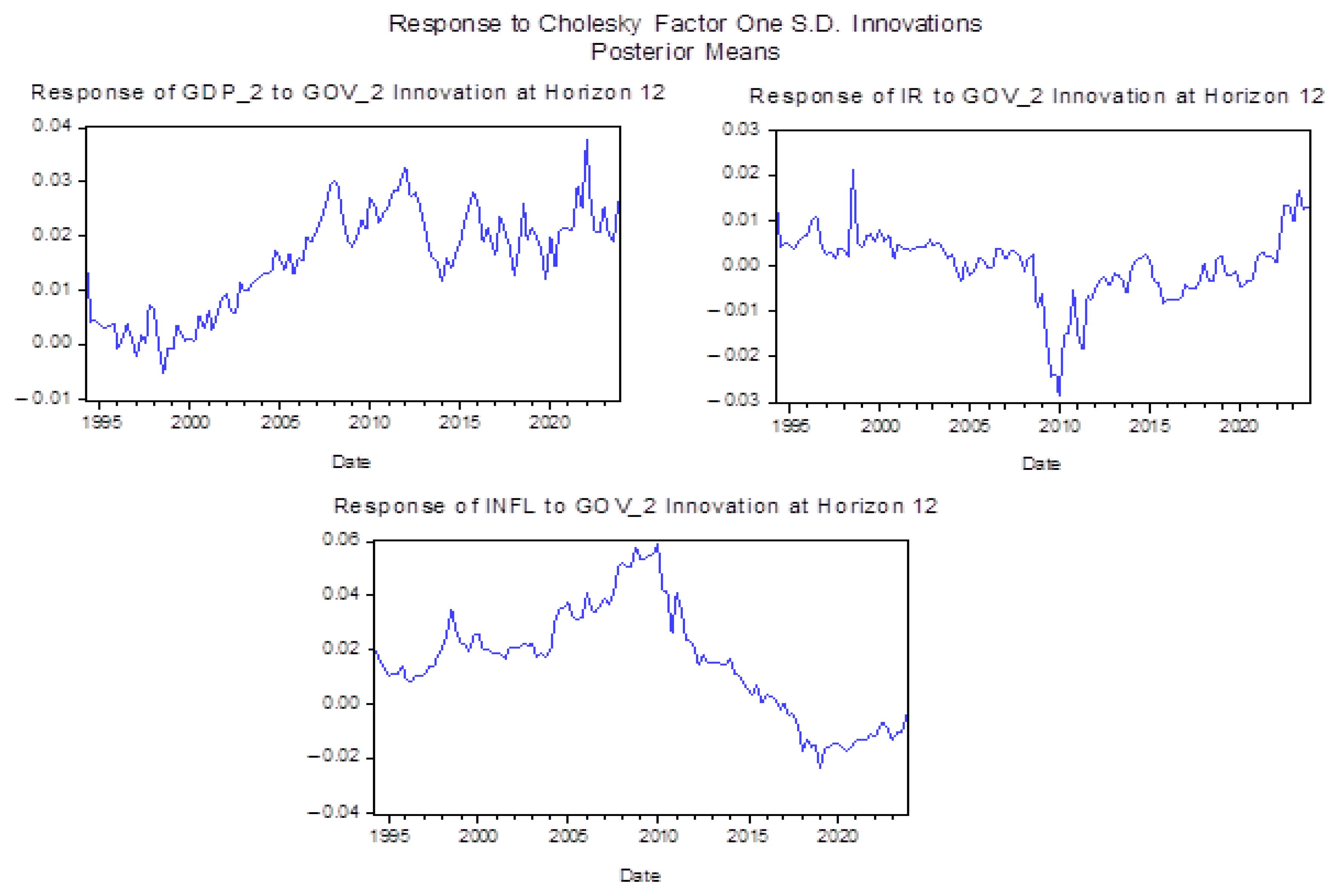
Figure 1 presents the time-varying impulse response to a positive government shock. In terms of GDP response to a fiscal expansion, it has, on average, seen increases over the years. A noticeable sharp decline was observed in 1998Q3, with the response being almost −0.01; this lasted for four consecutive quarters until a gradual increase in the response of GDP to government spending. This response aligns with empirical literature (SARB 1998; National Treasury of South Africa 1999), which attributes SA’s economic downturn to the Asian financial crisis and domestic structural challenges.
There is shift from a positive response of GDP in 1999 to a sharp decline in 2008 during the financial crisis. The highest responsiveness was in 2022, with a response of 0.04, showing a positive economic recovery after the COVID-19 economic shock. Regarding interest rates responding to a fiscal expansion, the response has been positive and dependent on the state of the economy. This can be seen in the highest positive response in 1998Q3, implying a countercyclical MP this year. Notably, interest rates in response to a fiscal expansion became more accommodative in 2010. After the 2008 global financial crisis, SA used fiscal stimulus to increase deficits. SARB kept interest rates low for a while to support growth.
Furthermore, during COVID-19 (2020–2021), interest rate responsiveness was accommodative; however, rising debt levels sparked concerns about long-term sustainability and future rate hikes. Regarding the inflation rate, the responsiveness of inflation to a fiscal expansion has been positive over the years, with a noticeable steady decline trend from 2010Q3. The lowest was 2019Q1 at –0.02. Although the response picked up a bit after 2019, it was gradual, emphasising that the response of inflation to a fiscal expansion in SA depends on economic conditions. With an active MP in SA that uses inflation targeting, a lack of coordination between MP and FP tends to neutralise the effects of a fiscal expansion.

4.1.2. Monetary Policy Shock

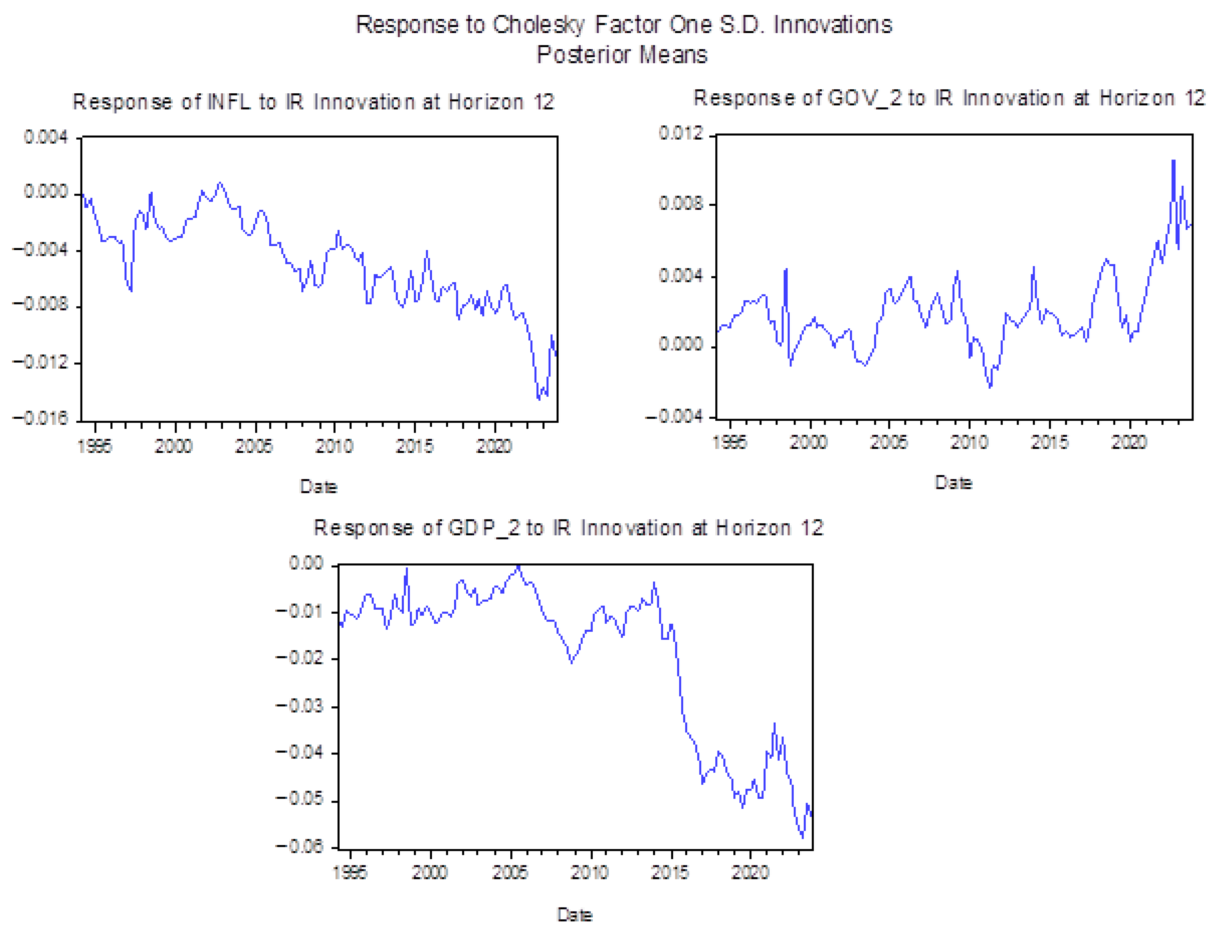
Figure 2 shows the time-varying impulse responses to a positive interest rate shock: a monetary expansion. The behaviour of inflation to monetary expansion is negative, with a sharp decline in inflation in 1997Q1. This negative relationship aligns with empirical literature, which states that the SARB uses the interest rates to curb inflation (Kabundi and Rapapali 2019). During the COVID-19 pandemic in 2020, SARB cut interest rates to stimulate the economy. While inflation was subdued during the early stages of the pandemic due to low demand, as the economy began to recover, inflationary pressures began to rise again (Burger and Calitz 2021). The relationship has been positive regarding government expenditure responses to an expansionary MP; however, it has been very volatile over the years, even though the response has been minimal.
A sharp increase in 1998Q3 can be attributed to the Asian and Russian financial crisis and the structural challenges that SA faced during that period. Furthermore, after adopting the inflation targeting framework in 2000, one can observe a steady increase in government expenditure as a response to a MP expansion. The effects of the GFC also saw a decline in government expenditure in response to a positive interest rate shock. Lastly, the relationship is negative in terms of GDP response to a positive interest rate shock. Implying that an expansionary MP may result in a decline in economic growth. Notably, the response of GDP to the interest rate declined between 2006Q1 and 2009Q3, which encompasses the effects of the GFC. There was an even greater decline in the response of GDP from 2015Q3 to 2017Q3. However, during COVID-19, there was a slight increase in GDP as it responded to the expansionary MP.
The overall results indicate that when dealing with a positive fiscal shock, there is a positive effect on output, with GDP increasing in response to government spending. However, this is not the case when the economy is in a crisis. The interest rate has been positive and state contingent, reflecting monetary accommodation specifically post-GFC and COVID-19. The findings of an expansionary MP indicate that inflation responds negatively to MP shocks, which aligns with the SARB’s inflation-targeting framework. Government expenditure displays a positive yet volatile response to a positive monetary shock, with notable spikes during periods of financial distress.
Additionally, GDP generally responds negatively to interest rate shocks. This aligns with the widely held view that MP effectively stimulates output in the short term, particularly through its influence on aggregate demand (Guth 2018). Overall, these findings suggest that FP in SA is highly dependent on external shocks and underscore the significance of strengthening MP and FP interactions in SA to enhance policy effectiveness.

4.2. The MSDR Analysis

To gain more insights into policy interactions, this study examines how MP and FP interact in the presence of potential regime changes. The MSDR framework captures regime and structural changes in these policies (Hamilton 1990). The FP and MP equations are specified by Equations (14) and (15).

4.2.1. Fiscal Policy

Results for the FP rule in regimes 1 and 2 are presented in Table 4. Regimes 1 and 2 are identified as passive FP, meaning that FP adjusts to ensure the government’s intertemporal budget constraint is satisfied for any path of the price level (Cochrane 2011). The dependent variable observed is government expenditure. The relationship between gross domestic product and government expenditure is statistically insignificant in both regimes. However, there is a positive relationship between GDP and government expenditure in the first regime and a negative relationship in the second regime. The coefficient of GDP is 0.484 in regime 1 and −0.513 in regime 2. These results underscore the empirical evidence within the South African context where the relationship between GDP and government expenditure tends to be positive in the short-run and can be negative in the long-run due to the presence of inefficiencies in government expenditure (Buthelezi and Nyatanga 2023; Buthelezi 2023).
The relationship between government expenditure and government debt is negative in both regimes, with the results being statistically insignificant at all levels in regime 1 and statistically significant at 10% in regime 2. The coefficients of the Debt-to-GDP ratio are −4.093 and −2.873 in regimes 1 and 2, respectively. These findings challenge existing evidence, which states that a positive relationship exists between Debt and government expenditure (Kharusi and Ada 2018). In South Africa, increased government expenditure has generally led to higher debt levels. However, persistently increasing debt levels have led to constrained spending, especially as pressures from credit rating agencies increase.
The inflation coefficients are 5.239 and 0.204 in regimes 1 and 2, respectively, indicating a statistically significant positive relationship between inflation and government spending in regime 1 and an insignificant relationship in regime 2. These results confirm empirical evidence which reflects a positive relationship between inflation and government expenditure within the South African context (Mazenda 2016). This positive relationship can be attributed to supply-side inefficiencies and challenges within the South African economy. The relationship between government expenditure and the interest rate is statistically significant at a 10% level in regime 1 and insignificant at all levels in regime 2. The interest rate coefficients are 0.111 and −0.008 in regimes 1 and 2, respectively. The relationship is positive in regime 1 and negative in regime 2. These findings confirm existing evidence of a positive relationship between government expenditure and the interest rate in South Africa (Bonga-Bonga and Mabejane 2009; Buthelezi 2023; SARB 2023).
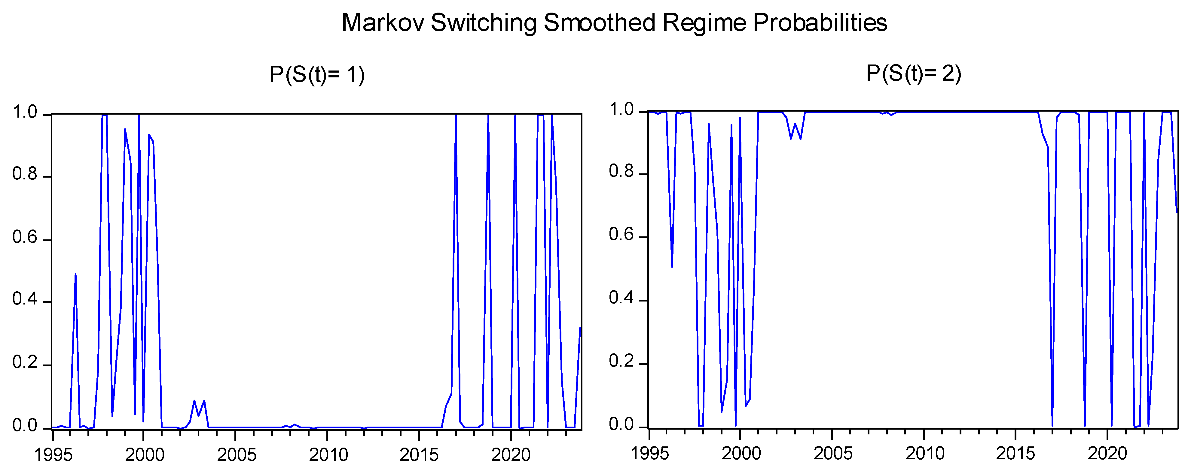
The study interprets the estimated transition matrix and the expected probabilities of FP regimes to gain insight into policy interactions. This provides insight into the stability and duration of different policy regimes.
The results of the transition matrix in Table 5 indicate that the probability of transitioning to Regime 1 given Regime 1 is 38.7%. This implies a lower tendency for the economy to remain in Regime 1 and a higher tendency to transition to Regime 2. Additionally, the probability of transitioning to Regime 2 given Regime 1 is 61.3%; this implies a higher tendency of the economy remaining in Regime 2. Furthermore, this implies that the resultant output of the optimal interaction between MP and FP performs better when the economy is in Regime 2. These findings align with economic policy evidence of South Africa following a mostly passive FP, with periods of attempted active FP in times of an economic crisis (National Treasury of South Africa 2023).
The probability of transitioning to Regime 1 given that the economy is in Regime 2 is 10%; this implies a higher tendency for the economy to remain in Regime 2. The probability of transitioning to Regime 2 given Regime 2 is 90%, implying a higher tendency for the economy to remain in Regime 2. Therefore, the results indicate that the resultant output of the optimal interaction between MP and FP of the government performs better in Regime 2 than in Regime 1. Overall, Regime 1 is less stable, with a low probability of the economy staying in this regime once it has entered. Regime 2 is more stable, with a high probability of the economy staying in this regime. Also, on average, the economy will stay in regime 1 for about 1.631 quarters before transitioning to regime 2. The expected time duration of regime 2 is on average 8.959, indicating that the economy tends to stay in regime 2 for about 8.956 quarters before switching back to regime 1 and suggesting that regime 2 represents a more stable economic condition for South Africa, while regime 1 is a more volatile state.
Figure 3 represents the regime switches of FP from 1994 to 2023. According to Leeper (1991), MP and FP must be consistent to sustain the policy rule; regime switches between fiscal and monetary rules should be synchronised. The figure below shows the perfect switch between regimes 1 and 2 for FP in South Africa.

4.2.2. Monetary Policy

Table 6 presents the results for the MP in regimes 1 and 2, indicating an active MP in both regimes. The dependent variable is the interest rate. The inflation rate behaviour in both regimes shows no significant relationship to the dependent variable, with the coefficients being 1.398 and 1.400, respectively. The positive relationship conforms to conventional theory, which states that a positive relationship exists between the interest rate and inflation. Particularly, within the South African context, findings by Kabundi and Mbelu (2018) suggest a positive but insignificant relationship between interest rates and inflation. This can be attributed to policy lags, expectation-based adjustments and socio-economic challenges the South African economy faces. The GDP coefficients are –12.909 in regime 1 and –15.491 in regime 2, indicating a statistically significant negative relationship between GDP and the interest rate in both regimes. The results confirm the conventional theory of a negative relationship between the two variables.
The empirical literature suggests that when the SARB increases interest rates to curb inflation, this results in slowed economic growth (SARB 2023; Meyer and Hassan 2024). The behaviour of government expenditure in both regimes indicates a positive and significant relationship between government expenditure and interest rates, with the coefficients being 0.540 and 0.594, respectively. The expected relationship is negative; these results challenge conventional theory. However, empirical evidence points to a positive relationship between the two variables within the South African context. This is linked to the cost of servicing debt, which increases government expenditure. According to the National Treasury of South Africa (2024), interest payments on debt have become one of the fastest-growing components of expenditure.
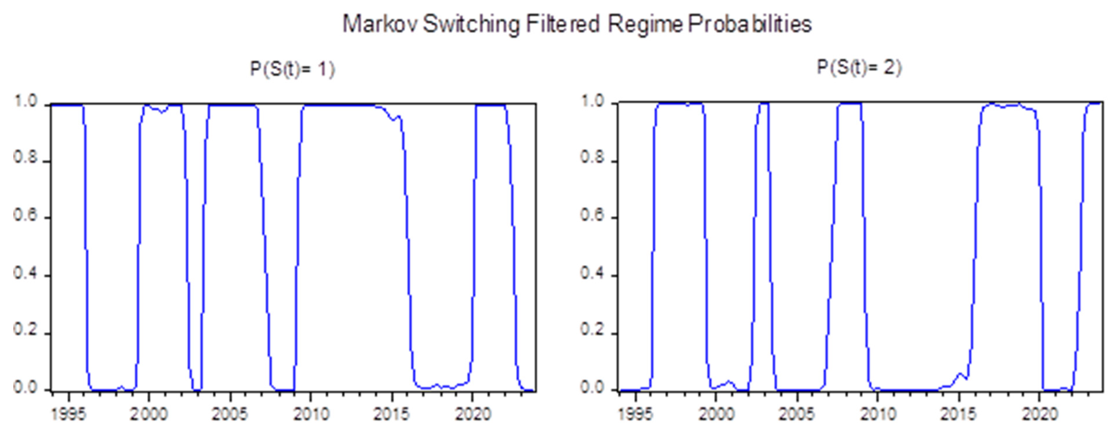
The results of the MP transition matrix are presented in Table 7. They indicate that the probability of transitioning to Regime 1 given Regime 1 is 93.3%. This implies a lower tendency for the economy to transition to Regime 2 and a higher tendency to remain in Regime 1. Additionally, the probability of transitioning to Regime 2 given Regime 1 is 6.7%; this implies a lower tendency for the economy to remain in Regime 2. The probability of transitioning to Regime 1 given that the economy is in Regime 2 is 9%; this implies a lower tendency for the economy to remain in Regime 2. The probability of transitioning to Regime 2 given Regime 2 is 91%, implying a higher tendency for the economy to remain in Regime 2. These findings align with economic policy evidence of South Africa following active MP (SARB 2023).
On average, the economy will stay in regime 1 for about 14.971 quarters before transitioning to regime 2. The expected time duration of regime 2 is on average 11.121, indicating that the economy tends to stay in regime 2 for about 11.121 quarters before switching back to regime 1. This suggests that both regimes are, on average, stable, with regime 1 being slightly longer than regime 2.
Figure 4 represents the regime switches of MP from 1994 to 2023. The figure below shows the perfect switch between regimes 1 and 2 for the South African MP.
Overall, the findings of the FP rule indicate that the relationship between government expenditure and GDP is statistically insignificant across both regimes. This suggests that while fiscal expansion may support economic growth in the short run, its effectiveness decreases in the long run. This may be due to the structural inefficiencies in government spending. Similarly, government expenditure shows a negative relationship between the two regimes. On the other hand, fiscal expansion raises inflation, especially given the persistent supply-side inefficiencies in SA. Interest rates exhibit a positive relationship to government spending during stable periods and are more accommodative in times of fiscal stress. The analysis of the MP rule indicates that Inflation shows a positive but statistically insignificant relationship with the interest rate in both regimes, consistent with South African literature suggesting that inflation targeting faces limitations due to policy lags and structural challenges. GDP exhibits a strong and statistically significant negative relationship with interest rates in both regimes, supporting conventional theory that tighter MP slows economic growth. Interestingly, government expenditure shows a positive and significant relationship with interest rates in both regimes. This contradicts standard expectations but aligns with South African evidence linking this to the rising debt servicing cost. These findings underscore the need for improved spending efficiency in SA and highlight the complexity of MP transition in SA. Given the economic landscape, which is faced with persistent fiscal constraints, credibility concerns, and structural inefficiencies,

5. Conclusions

This study attempts to understand the characteristics of South Africa’s MP and FP interactions. Using the TVP-VAR model and the MSDR, we model these interactions and attempt to identify any potential changes in policy interactions under different regimes. The main findings from the TVP-VAR model analysis indicate that GDP persists in response to a fiscal expansion, except during the 2008 GFC and COVID-19 pandemic, suggesting crowding-out effects during economic crises. This can be attributed to SA’s high debt levels and ongoing supply shocks. Contrary to conventional theory, the findings suggest that a fiscal expansion reduces inflation. These results align with Buthelezi (2024), who finds a decrease in CPI following a fiscal expansion. These findings reflect anchored inflation expectations, especially with the adoption of the inflation-targeting framework in SA. Conversely, the effects of a monetary expansion on GDP can be attributed to structural supply constraints and capital flight due to a loss of business confidence.
Furthermore, inflation exhibits a weak response to IR shocks, suggesting MP ineffectiveness during liquidity traps. The main findings from the MSDR analysis indicate that SA MP is active, while FP is passive. There is also a higher tendency for the economy to be in a state where MP is active and FP is passive. However, the interest rate and government expenditure exhibit a positive relationship, challenging conventional theory and alluding to fiscal dominance risks in SA.
These results necessitate understanding the characteristics of MP and FP to make informed policy decisions in dealing with unexpected economic shocks. The fiscal expansion and CPI relationship suggests that fiscal stimulus measures may fail to stimulate demand in SA. The recommendation is for much more targeted government spending, focusing on infrastructure investment. Additionally, passive FP and active MP limit policy effectiveness during economic downturns. The recommendation would be higher levels of policy coordination during economic downturns and policy design which is more regime aware, especially within SA’s volatile economic environment. While this paper furthers the understanding of MP and FP interactions, Further research can attempt to analyse the structural factors within SA that hinder the achievement of an optimal policy mix.
Author Contributions

Conceptualization A.M., M.C.N. and S.M.; methodology, A.M., M.C.N. and S.M.; validation, A.M.; formal analysis A.M., M.C.N. and S.M.; investigation, A.M., M.C.N. and S.M.; resources, A.M., M.C.N. and S.M.; data curation, A.M., M.C.N. and S.M.; writing—original draft preparation, A.M., M.C.N. and S.M.; writing—review, A.M., M.C.N. and S.M.; visualization, A.M. supervision, M.C.N. and S.M. All authors have read and agreed to the published version of the manuscript.

Funding

This research received no external funding.

Data Availability Statement

The data presented in this study are openly available in the South African Reserve Bank repository. [SARB] [https://www.resbank.co.za/en/home] (accessed on 3 June 2025).

Conflicts of Interest

The authors declare no conflict of interest.

References

  1. Afonso, António, and Alexandre Sousa. 2020. The Interplay Between Monetary and Fiscal Policies in the EU. Lisboa: Universidade de Lisboa. [Google Scholar]
  2. Afonso, António, and Luis Gonçalves. 2020. The policy mix in the US and EMU: Evidence from a SVAR analysis. The North American Journal of Economics and Finance 51: 100840. [Google Scholar] [CrossRef]
  3. Arby, Muhammad Farooq, and Muhammad Nadeem Hanif. 2010. Monetary and Fiscal Policies Coordination-Pakistan’s Experience. München: University Library of Munich. [Google Scholar]
  4. Aruoba, S. Borağan, and Thomas Drechsel. 2024. The long and variable lags of monetary policy: Evidence from disaggregated price indices. Journal of Monetary Economics 148: 103635. [Google Scholar] [CrossRef]
  5. Ascari, Guido, Anna Florio, and Alessandro Gobbi. 2020. Monetary-fiscal interactions under price level targeting. arXiv arXiv:2010.14979. [Google Scholar] [CrossRef]
  6. Auerbach, Alan J., Yuriy Gorodnichenko, and Daniel Murphy. 2021. Inequality, fiscal policy and COVID19 restrictions in a demand-determined economy. European Economic Review 137: 103810. [Google Scholar] [CrossRef]
  7. Banerjee, Anindya, and Sheheryar Malik. 2012. The Changing Role of Expectations in US Monetary Policy: A New Look Using the Livingston Survey. Paris: Banque de France, No. 376. [Google Scholar]
  8. Barro, Robert J., and Francesco Bianchi. 2023. Fiscal Influences on Inflation in OECD Countries, 2020–2023. Cambridge: National Bureau of Economic Research, No. w31838. [Google Scholar]
  9. Bassetto, Marco, and Thomas J. Sargent. 2020. Shotgun wedding: Fiscal and monetary policy. Annual Review of Economics 12: 659–90. [Google Scholar] [CrossRef]
  10. Bianchi, Francesco, and Leonardo Melosi. 2017. Escaping the great recession. American Economic Review 107: 1030–58. [Google Scholar] [CrossRef]
  11. Blanchard, Olivier. 2019. Public debt and low interest rates. American Economic Review 109: 1197–229. [Google Scholar] [CrossRef]
  12. Bohn, Henning. 1998. The behavior of US public debt and deficits. The Quarterly Journal of Economics 113: 949–63. [Google Scholar] [CrossRef]
  13. Bonga-Bonga, Lumengo, and John Mabejane. 2009. Budget deficit, long-term interest rates and crowding-out effect in South Africa. Discourse 37: 28–38. [Google Scholar]
  14. Burger, Philippe, and Estian Calitz. 2021. COVID-19, economic growth and South African fiscal policy. South African Journal of Economics 89: 3–24. [Google Scholar] [CrossRef]
  15. Buthelezi, Eugene M., and Phocenah Nyatanga. 2023. The dynamic relationship between government debt, fiscal consolidation, and economic growth in South Africa: A threshold analysis. Cogent Economics & Finance 11: 2261329. [Google Scholar] [CrossRef]
  16. Buthelezi, Eugene Msizi. 2023. Examining the dynamic nexus of monetary and fiscal policy in South Africa: Evidence from key macroeconomic economic indicators. Journal of Economics and Financial Analysis 7: 13–42. [Google Scholar]
  17. Buthelezi, Eugene Msizi. 2024. South African inflation response to fiscal policy shocks. Journal of Applied Economics 27: 2381168. [Google Scholar] [CrossRef]
  18. Büyükbaşaran, Tayyar, Cem Cebi, and Erdal Yılmaz. 2020. Interaction of monetary and fiscal policies in Turkey. Central Bank Review 20: 193–203. [Google Scholar] [CrossRef]
  19. Canzoneri, Matthew B., Robert E. Cumby, and Behzad Diba. 2003. New views on the transatlantic transmission of fiscal policy and macroeconomic policy coordination. In Monetary and Fiscal Policies in EMU. Leeds: Emerald Publishing, pp. 283–311. [Google Scholar]
  20. Cevik, Emrah Ismail, Sel Dibooglu, and Ali M. Kutan. 2014. Monetary and fiscal policy interactions: Evidence from emerging European economies. Journal of Comparative Economics 42: 1079–91. [Google Scholar] [CrossRef]
  21. Chibi, Abderrahim, Sidi Mohamed Chekouri, and Mohamed Benbouziane. 2019. The dynamics of fiscal policy in Algeria: Sustainability and structural change. Journal of Economic Structures 8: 28. [Google Scholar] [CrossRef]
  22. Chibi, Abderrahim, Youcef Zahaf, and Sidi Mohammed Chekouri. 2024. Strategic Interaction Between Monetary and Fiscal Policy in Algeria: A Game Theory Approach. International Journal of Business and Economic Studies 6: 262–80. [Google Scholar] [CrossRef]
  23. Claeys, Peter. 2004. Monetary and Budgetary Policy Interaction: An SVAR Analysis of Stabilisation Policies in Monetary Union. Fiesole: European University Institute. [Google Scholar]
  24. Cochrane, John H. 2001. Long-term debt and optimal policy in the fiscal theory of the price level. Econometrica 69: 69–116. [Google Scholar] [CrossRef]
  25. Cochrane, John H. 2011. Understanding policy in the Great Recession: Some unpleasant fiscal arithmetic. European Economic Review 55: 2–30. [Google Scholar] [CrossRef]
  26. Cochrane, John H. 2021. The Fiscal Theory of the Price Level: An Introduction and Overview. Journal of Economic Perspectives. Available online: https://www.johnhcochrane.com/s/Fiscal_theory_JEP.pdf (accessed on 3 June 2025).
  27. Corsetti, Giancarlo, Luca Dedola, Marek Jarociński, Bartosz Maćkowiak, and Sebastian Schmidt. 2019. Macroeconomic stabilization, monetary-fiscal interactions, and Europe’s monetary union. European Journal of Political Economy 57: 22–33. [Google Scholar] [CrossRef]
  28. da Silva, Cleomar Gomes, and Flávio Vilela Vieira. 2017. Monetary and fiscal policy in advanced and developing countries: An analysis before and after the financial crisis. The Quarterly Review of Economics and Finance 63: 13–20. [Google Scholar] [CrossRef]
  29. Davig, Troy, Eric M. Leeper, Richard H. Clarida, and Jesper Lindé. 2006. Endogenous monetary policy regime change [with comments]. In NBER International Seminar on Macroeconomics. Chicago: The University of Chicago Press, vol. 2006, No. 1, pp. 345–91. [Google Scholar]
  30. Dixit, Avinash, and Luisa Lambertini. 2003. Interactions of commitment and discretion in monetary and fiscal policies. American Economic Review 93: 1522–42. [Google Scholar] [CrossRef]
  31. Du Plessis, Stan, Ben Smit, and Federico Sturzenegger. 2007. The cyclicality of monetary and fiscal policy in South Africa since 1994. South African Journal of Economics 75: 391–411. [Google Scholar] [CrossRef]
  32. Goldfeld, Stephen M., and Richard E. Quandt. 1973. A Markov model for switching regressions. Journal of Econometrics 1: 3–15. [Google Scholar] [CrossRef]
  33. Guth, Martin. 2018. Heterogeneous Effects of Unconventional Monetary Policy on Loan Demand and Supply. Insights from the Bank Lending Survey. arXiv arXiv:1807.04161. [Google Scholar] [CrossRef]
  34. Hamilton, James D. 1989. A New Approach to the Economic Analysis of Non-stationary Time Series and the Business Cycle. Econometrica 57: 357–84. [Google Scholar] [CrossRef]
  35. Hamilton, James D. 1990. Analysis of Time Series Subject to Changes in Regime. Journal of Econometrics 45: 39–70. [Google Scholar] [CrossRef]
  36. Hammoudeh, Shawkat, Duc Khuong Nguyen, and Ricardo M. Sousa. 2015. US monetary policy and sectoral commodity prices. Journal of International Money and Finance 57: 61–85. [Google Scholar] [CrossRef]
  37. Heijmans, Roweno J. 2023. Unraveling coordination problems. arXiv arXiv:2307.08557. [Google Scholar] [CrossRef]
  38. Hooley, John, Lam Nguyen, Mika Saito, and Shirin Nikaein Towfighian. 2021. Fiscal Dominance in Sub-Saharan Africa Revisited. Washington, DC: International Monetary Fund. [Google Scholar]
  39. IMF. 2023. World Economic Outlook: Navigating Global Divergences. Washington, DC: International Monetary Fund. [Google Scholar]
  40. Jordà, Òscar, Sanjay R. Singh, and Alan M. Taylor. 2023. Does Monetary Policy Have Long-Run Effects? FRBSF Economic Letter 2023: 1–6. [Google Scholar]
  41. Kabundi, Alain, and Asi Mbelu. 2018. Has the exchange rate pass-through changed in South Africa? South African Journal of Economics 86: 339–60. [Google Scholar] [CrossRef]
  42. Kabundi, Alain, and Mpho Rapapali. 2019. The transmission of monetary policy in South Africa before and after the global financial crisis. South African Journal of Economics 87: 464–89. [Google Scholar] [CrossRef]
  43. Kharusi, Sami Al, and Mbah Stella Ada. 2018. External debt and economic growth: The case of emerging economy. Journal of economic integration 33: 1141–57. [Google Scholar] [CrossRef]
  44. Leeper, Eric M. 1991. Equilibria under ‘active’ and ‘passive’ monetary and fiscal policies. Journal of Monetary Economics 27: 129–47. [Google Scholar] [CrossRef]
  45. Leshoro, Temitope L. A. 2020. Monetary policy or fiscal policy, which one better explains inflation dynamics in South Africa? African Journal of Business & Economic Research 15: 27–52. [Google Scholar]
  46. Maitra, Biswajit, and Tafajul Hossain. 2025. Assessing Sectoral Growth Impact of Public Expenditure in India. Journal of Quantitative Economics, 1–26. [Google Scholar] [CrossRef]
  47. Majenge, Luyanda, Sakhile Mpungose, and Simiso Msomi. 2024. Econometric Analysis of South Africa’s Fiscal and Monetary Policy Effects on Economic Growth from 1980 to 2022. Economies 12: 227. [Google Scholar] [CrossRef]
  48. Mazenda, Adrino. 2016. The Effect of BRICS Trade Relations on South Africa’s Growth. EERI Research Paper Series, No. 11/2016; Brussels: Economics and Econometrics Research Institute (EERI). [Google Scholar]
  49. Meyer, Daniel Francois, and Adewale Samuel Hassan. 2024. Analysis of the optimal inflation rate in the economic growth process of a developing country: The case of South Africa. Journal of Infrastructure, Policy and Development 8: 3607. [Google Scholar] [CrossRef]
  50. Mishra, Prachi, Peter J. Montiel, and Antonio Spilimbergo. 2012. Monetary transmission in low-income countries: Effectiveness and policy implications. IMF Economic Review 60: 270–302. [Google Scholar] [CrossRef]
  51. Nakajima, Jouchi. 2011. Time-varying parameter VAR model with stochastic volatility: An overview of methodology and empirical applications. Monetary and Economic Studies 29: 107–42. [Google Scholar]
  52. Nasrullah, Muhammad Junaid, Ghulam Saghir, Muhammad shahid Iqbal, and Phool Hussain. 2023. Macroeconomic Stability and Optimal Policy Mix. iRASD Journal of Economics 5: 725–45. [Google Scholar] [CrossRef]
  53. National Treasury of South Africa. 1999. Annual Report 1999; Pretoria: Department of Finance. Available online: https://www.treasury.gov.za/publications/annual%20reports/national%20treasury/nt%20annual%20report%201999.pdf (accessed on 3 June 2025).
  54. National Treasury of South Africa. 2023. Budget Review 2023; Pretoria: National Treasury. Available online: https://www.treasury.gov.za (accessed on 18 November 2024).
  55. National Treasury of South Africa. 2024. Budget Review 2024. Pretoria: National Treasury. [Google Scholar]
  56. Oboh, Victor Ugbem. 2017. Monetary and fiscal policy coordination in Nigeria: A set theoretic approach. Academic Journal of Economic Studies 3: 48–58. [Google Scholar]
  57. Ocran, Matthew Kofi. 2019. Economic Development in the Twenty-First Century: Lessons for Africa Throughout History. London: Palgrave Macmillan. [Google Scholar]
  58. Primiceri, Giorgio E. 2005. Time Varying Structural Vector Autoregressions and Monetary Policy. Review of Economic Studies 72: 821–52. [Google Scholar] [CrossRef]
  59. Quandt, Richard E. 1972. A New Approach to Estimating Switching Regressions. Journal of the American Statistical Association 67: 306–10. [Google Scholar] [CrossRef]
  60. Reis, Ricardo. 2023. What can keep euro area inflation high? Economic Policy 38: 495–517. [Google Scholar] [CrossRef]
  61. Sangweni, Sinethemba D., and Harold Ngalawa. 2023. Inflation dynamics in South Africa: The role of public debt. Journal of Economic and Financial Sciences 16: 750. [Google Scholar] [CrossRef]
  62. Shvets, Serhii. 2023. Dominance score in the fiscal-monetary interaction. National Accounting Review 5: 186–207. [Google Scholar] [CrossRef]
  63. Sims, Christopher A. 1980. Macroeconomics and reality. Econometrica: Journal of the Econometric Society 48: 1–48. [Google Scholar]
  64. Sims, Christopher A. 1994. A simple model for study of the determination of the price level and the interaction of monetary and fiscal policy. Economic Theory 4: 381–99. [Google Scholar] [CrossRef]
  65. South African Reserve Bank (SARB). 1998. Annual Report 1998. Pretoria: South African Reserve Bank. [Google Scholar]
  66. South African Reserve Bank (SARB). 2023. Monetary Policy Review. Pretoria: SARB. Available online: https://www.resbank.co.za (accessed on 16 November 2024).
  67. Šehović, Damir. 2013. General aspects of monetary and fiscal policy coordination. Journal of Central Banking Theory and Practice 2: 5–27. [Google Scholar]
  68. Tuncer, Güner, and Adil Akıncı. 2018. Effectiveness of fiscal policy and monetary policy in Turkey. Dumlupınar Üniversitesi Sosyal Bilimler Dergisi 57: 120–8. [Google Scholar]
  69. Woodford, Michael. 1995. Price-level determinacy without control of a monetary aggregate. In Carnegie-Rochester Conference Series on Public Policy. Amsterdam: North-Holland, Vol. 43, pp. 1–46. [Google Scholar]
  70. Zhang, Enqi. 2024. Coordination of Monetary and Fiscal Policies from a Game Theoretic Perspective. Advances in Economics, Management and Political Sciences 107: 10–14. [Google Scholar] [CrossRef]
Figure 1. Response to a Government Spending Shock. Source: Author’s computation, Data sourced from SARB.
Risks 13 00185 g001
Figure 2. Response to an Interest rate Shock. Source: Author’s computation, Data sourced from SARB.
Risks 13 00185 g002
Figure 3. The filtered transition probabilities for regimes 1 and 2 (Fiscal Policy). Source: Author’s computation, Data sourced from SARB.
Risks 13 00185 g003
Figure 4. The filtered transition probabilities for regimes 1 and 2 (Monetary Policy). Source: Author’s computation, Data sourced from SARB.
Risks 13 00185 g004
Table 1. Unit root test results.
Variablet-Statisticp-Value
Gross Domestic Product−10.18760.0000
Government expenditure−8.36950.0000
Inflation−6.10490.0000
Interest rate−8.01540.0000
Debt/GDP−8.18810.0000
Source: Own calculations, Data sourced from SARB.
Table 2. Lag Selection Results.
LagAICSCHQ
03.7173.8143.757
1−2.277−1.791 *−2.080
2−2.475−1.602−2.121 *
3−2.523−1.261−2.011
4−2.569−0.919−1.899
5−2.441−0.403−1.614
6−2.860−0.433−1.875
7−2.996−0.180−1.853
8−3.009 *0.195−1.709
Key: * indicates the optimal hysteresis order determined by the corresponding method. Source: Author’s computation, Data sourced from SARB.
Table 3. TVP-VAR model estimation results.
Estimation Results
ParameterMeanStdev95%L95%UGewekeInef
Sb1−0.4020.045−0.472−0.2840.9526.734
Sb2−0.0070.008−0.0290.004−1.0684.558
Sa10.0070.014−0.0300.026−1.2546.474
Sa20.0490.062−0.0280.1961.0483.359
Sh10.2810.1330.0800.5450.4793.277
Sh20.1840.0550.0940.2920.3743.633
Key: Mean denotes the posterior mean; Stdev denotes the standard deviation; and Inef. denotes the inefficiency factor. Source: Author’s computation, Data sourced from SARB.
Table 4. Markov Switching Regression Results: Fiscal Policy.
Dependent Variable: Government Expenditure
Regime 1: Passive FPRegime 2: Passive FP
Coeff.SEp-valueCoeff.SEp-value
C−22.36216.0550.1648.887 *1.7000.089
GDP0.4841.1010.660−0.5130.3630.158
Debt−4.0934.3100.342−2.873 *1.5130.058
inf5.239 ***1.9350.0070.2040.4560.655
ir0.111 *0.0600.066−0.0080.0230.726
q−1.0180.078 −13.0760.000
Key: *** Significant at 1%, ** Significant at 5%, * Significant at 10%. Source: Author’s computation, Data sourced from SARB.
Table 5. Matrix of the transition and expected probabilities of fiscal policy regimes.
12
10.3870.613
20.1000.90
All periods1.6319.956
Source: Author’s computation.
Table 6. Markov Switching Regression Results: Monetary Policy Rule.
Dependent Variable: Interest Rate
Regime 1: Active MPRegime 2: Active MP
Coeff.SEp-valueCoeff.SEp-value
C179.060 ***11.4730.000217.698 ***9.2440.000
Infl1.3982.8180.6201.4001.4350.330
GDP−12.909 ***0.6360.000−15.491 ***0.6520.000
Gov. exp0.540 **0.2200.0140.594 **0.2790.033
q2.6370.498 −2.3150.513
Key: *** Significant at 1%, ** Significant at 5%, * Significant at 10%. Source: Author’s computation, Data sourced from SARB.
Table 7. Matrix of the transition and expected probabilities of Monetary policy regimes.
12
10.9330.067
20.0900.910
All periods14.97111.121
Source: Author’s computation, Data sourced from SARB.
Disclaimer/Publisher’s Note: The statements, opinions and data contained in all publications are solely those of the individual author(s) and contributor(s) and not of MDPI and/or the editor(s). MDPI and/or the editor(s) disclaim responsibility for any injury to people or property resulting from any ideas, methods, instructions or products referred to in the content.