Claim Prediction and Premium Pricing for Telematics Auto Insurance Data Using Poisson Regression with Lasso Regularisation


Abstract
1. Introduction
2. Methodologies
2.1. Regression Models
2.1.1. Poisson Regression Model
2.1.2. Poisson Mixture Model
2.2. Regularisation Techniques
2.3. Model Performance Measures
3. Empirical Studies
3.1. Data Description
3.2. Data Cleaning and DVs Setting
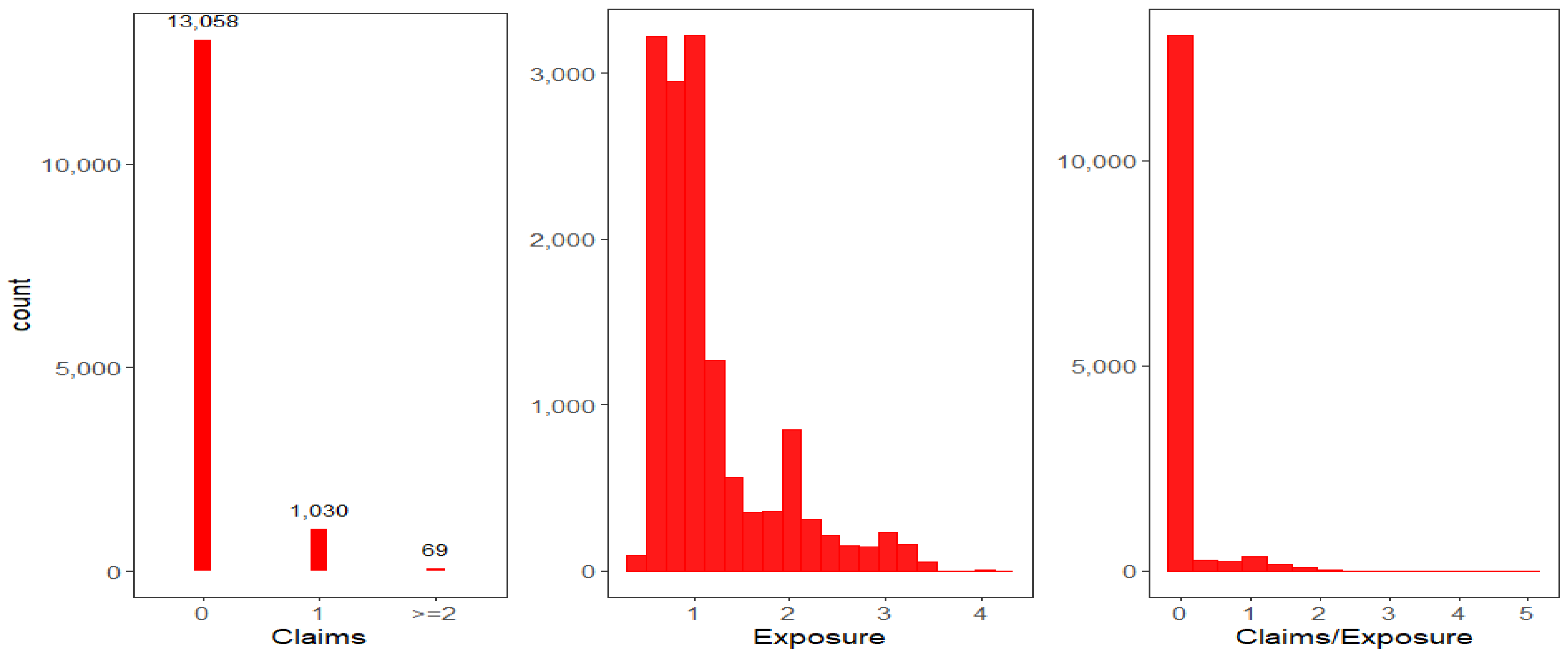
3.3. Exploratory Data Analyses
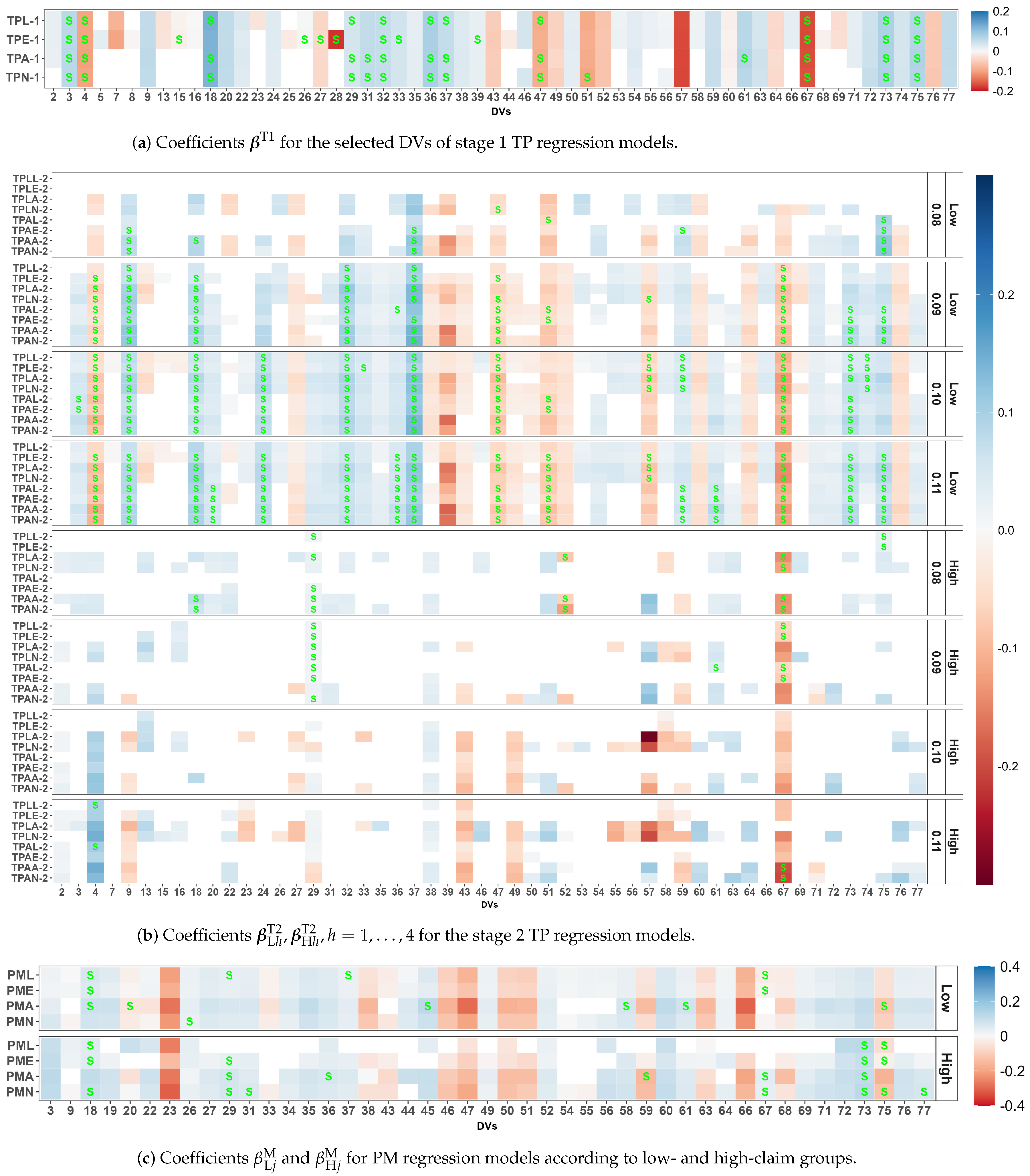
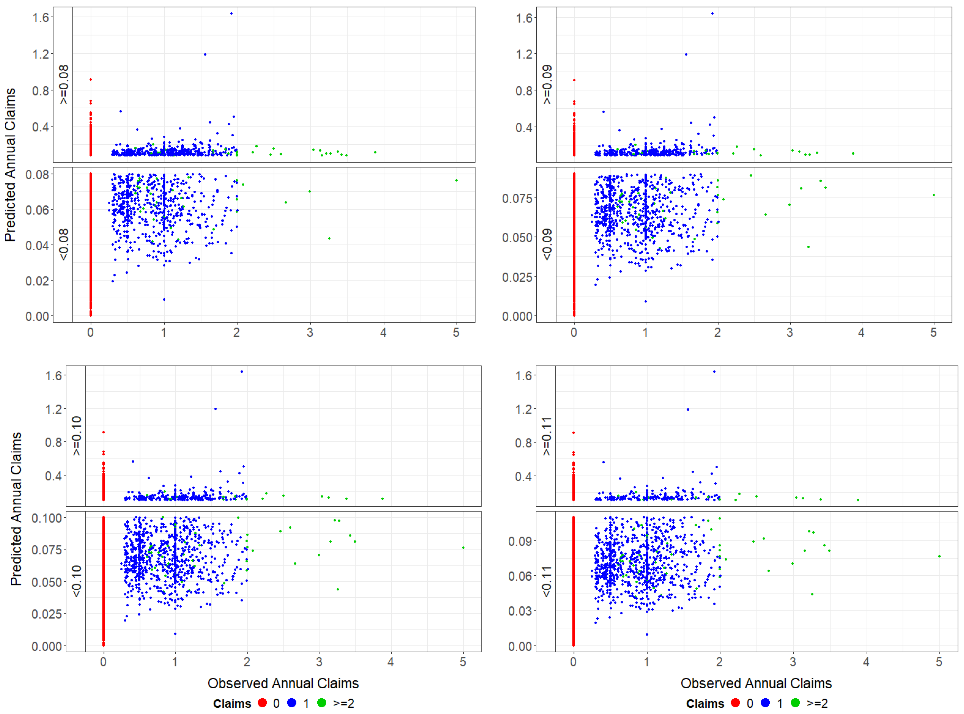
3.4. Two-Stage Threshold Poisson Model

 |
3.5. Poisson Mixture Model
3.6. Zero-Inflated Poisson Model
3.7. Model Comparison and Selection
4. UBI Experience Rating Premium
5. Conclusions
Author Contributions
Funding
Data Availability Statement
Conflicts of Interest
Abbreviations
| A | Adaptive lasso |
| AIC | Akaike information criterion |
| BIC | Bayesian information criterion |
| DVs | Driver behaviour variables |
| E | Elastic net |
| GLM | Generalized linear model |
| GPS | Global positioning system |
| IG | Information gain |
| L | Lasso |
| MSE | Mean squared error |
| N | Adaptive elastic net |
| NB | Negative binomial |
| PAYD | Pay As You Drive |
| PHYD | Pay How You Drive |
| PM | Poisson mixture |
| RMSE | Root mean squared error |
| ROC | Receiver operating characteristic curve |
| TP | Two-stage threshold Poisson |
| UBI | Usage-based auto insurance |
| ZIP | Zero-inflated Poisson |
Appendix A. Details of Stage 1 TP Model Procedures
- Draw subsamples with each containing drivers, where the index set contains all i being sampled. The K-fold CV () further splits into 10 nonoverlapping and equal-sized () CV setsand the training sets are , with index set . Set for some M to be the list of potential .
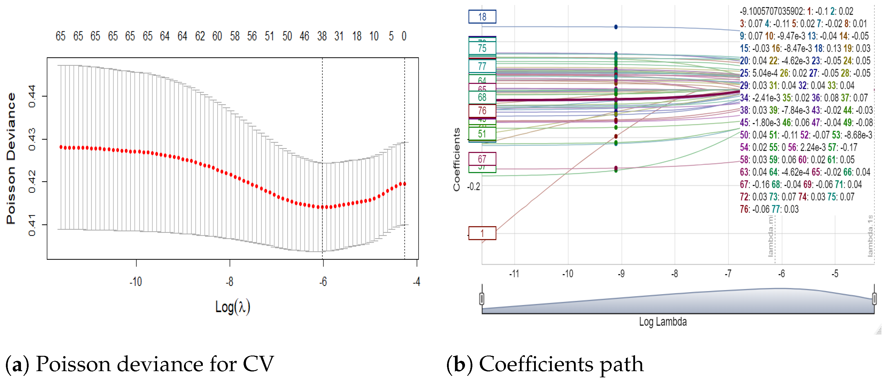
- Estimate in (7) for each and training set at repeat r and CV k. Find optimal that minimises some regularised CV test statistic such as MSE, MAE, or Deviance (Dev). Taking Dev as an example,where the mean . Among MSE, MAE, and Dev statistics, optimal using Dev is selected according to the RMSE of predicted claims for all subsamples. Using , is re-estimated based on the subsample . Figure A1a plots Poisson deviance with SE against , showing how it drops to for the first subsample (). Figure A1b shows how shrinks to zero as increases.
- Average those nonzero coefficients (selected at least once) over repeats as below:where is the indicator function of event A, and the index setcontains those DVs selected at least once over R subsamples in stage 1. The averaged coefficients (based on Dev) are reported in Table A2 for the TPL-1 and TPA-1 models using the optimal . For example, DV 10 is not even selected once for the TPL-1 model.
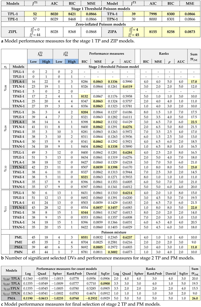
- Further select DVs that are frequently (not rarely) selected according to a weighted selection frequency measure given byweighting inversely to RMSEr. Superscripts T1, T2, M, and Z are added to when applied to the stage 1 TP, stage 2 TP, PM, and ZIP models, respectively. This weighted selection counts using MSE, MAE, and deviance, which are also reported in Table A2 for the TPL-1 and TPA-1 models. Table 3a shows that the TPL-1 and TPA-1 models have been selected according to the model performance measures AIC, BIC, and MSE. The results of the TPL-1 model in Table A2 show that 12 DVs in deep grey highlight with have been dropped, as they are rarely selected, resulting in DVs. These DVs can be interpreted as frequently selected DVs or simply selected DVs.
Appendix B. Some Technical Details of Model Implementation
- This study utilises R commands glm to fit Poisson regression and glmnet to fix Poisson regression with lasso regularisation (Zeileis et al. 2008). The latter command begins with adopting the R function sparse.model.matrix asdata_feature <- sparse.model.matrix(∼., dt_feature).We use the argument penalty.factor in cv.glmnet for adaptive lasso. We remark that the glmnet package does not provide a p value. We extract the p value for the selected DVs by refitting the model using glm procedure.
- We use the 100 simulated dataset in stages 1 and 2 of the TP and PM models to explore optimal values in the elastic net. We first set up our 10-fold CV strategy. Using caret package in R, we use train() with method = “glmnet” to fit the elastic net.XX = model.matrix(Claims ~ . -EXP-1,data=stage1)YY = stage1$ClaimsOFF = log(stage1$EXP)Fit_stage1 <- caret::train(x = cbind(XX,OFF),y = YY,method = "glmnet",family = "poisson",tuneLength = 10,trControl = trainControl(method="cv", number = 10, repeats = 100))
- We use roc() in the pROC package to calculate the AUC. The latex2exp package also provides an ROC plot.
- We implement the AER package in R using the built-in command dispersiontest() that assesses the alternative hypothesis , where the transformation function (by default, trafo = NULL) corresponds to the Poisson model with . If the dispersion is greater than 1, it indicates overdispersion.
- The PM regression model is estimated usingFLXMRglmnet(formula = .∼., family = c("gaussian","binomial","poisson"),adaptive = TRUE, select = TRUE, offset = NULL, …)in the R package flexmix (Leisch 2004) to fit mixtures of GLMs with lasso regularisation. Setting adaptive = TRUE for the adaptive lasso triggers a two-step process. Initially, an unpenalised model is fitted to obtain the preliminary coefficient estimates for the penalty weights .Then, values are applied to each coefficient in the subsequent model fitting. With the selected DVs for the low- and high-claim groups, FLXMRglmfix() refits the model, provides the significance of the coefficients, predicts claims, supports CV values and evaluates various goodness-of-fit measures.
- The ZIP regression model is estimated using the zipath() function for lasso and elastic net regularisation and the ALasso() function for adaptive lasso regularisation from the mpath and AMAZonn packages. The optimal lambda minimum is searched via 10-fold cross-validation with cv.zipath() and applied to both fitted models, ZIPL and ZIPA, for subsamples, each with 70% data. Full data are refitted to the PM model based on the selected DVs using Poisson zeroinf.
Appendix C. Driving Variable Description
| Event type | ||
| ACC | Acceleration Event—Accelerating/From full stop | |
| C1 | Smooth acceleration (acceleration to 30 MPH in more than 12 s) | |
| C2 | Moderate acceleration (acceleration to 30 MPH in 5–11 s) | |
| BRK | Braking Event—Full Stop/Slow down | |
| C1 | Smooth, even slowing down (up to about 7 mph/s) | |
| C2 | Mild to sharp brakes with adequate visibility and road grip (7–10 mph/s) | |
| LFT | Left turning Event—None (Interchange, curved road, overtaking)/At Junction | |
| C1 | Smooth, even cornering within the posted speed and according to the road and visibility conditions | |
| C2 | Moderate cornering slightly above the posted speed (cornering with light disturbance to passengers) | |
| RHT | Right turning Event—None (Interchange, curved road, overtaking)/At Junction | |
| C1 and C2 are the same as LFT | ||
| Time type | |
| T1 | Weekday late evening, night, midnight, early morning |
| T2 | Weekday morning rusk, noon, afternoon rush |
| T3 | Weekday morning, afternoon, no rush |
| T4 | Friday rush |
| T5 | Weekend night |
| T6 | Weekend day |
| DV1 | ACC_ACCELERATING_T3_C1 | DV19 | BRK_FULLSTOP_T1_C1 | DV39 | LFT_NONE_T1_C1 | DV57 | RHT_NONE_T1_C1 |
| DV2 | ACC_ACCELERATING_T3_C2 | DV20 | BRK_FULLSTOP_T1_C2 | DV43 | LFT_NONE_T6_C1 | DV58 | RHT_NONE_T1_C2 |
| DV3 | ACC_ACCELERATING_T4_C1 | DV22 | BRK_FULLSTOP_T2_C2 | DV44 | LFT_NONE_T6_C2 | DV59 | RHT_NONE_T4_C1 |
| DV4 | ACC_ACCELERATING_T4_C2 | DV23 | BRK_FULLSTOP_T3_C1 | DV45 | LFT_ATJUNCTION_T1_C1 | DV60 | RHT_NONE_T4_C2 |
| DV5 | ACC_ACCELERATING_T5_C1 | DV24 | BRK_FULLSTOP_T3_C2 | DV46 | LFT_ATJUNCTION_T1_C2 | DV61 | RHT_NONE_T5_C1 |
| DV7 | ACC_ACCELERATING_T5_C2 | DV25 | BRK_FULLSTOP_T4_C1 | DV47 | LFT_ATJUNCTION_T2_C1 | DV63 | RHT_NONE_T5_C2 |
| DV8 | ACC_FROMFULLSTOP_T1_C1 | DV26 | BRK_FULLSTOP_T4_C2 | DV49 | LFT_ATJUNCTION_T3_C1 | DV64 | RHT_NONE_T6_C1 |
| DV9 | ACC_FROMFULLSTOP_T1_C2 | DV27 | BRK_FULLSTOP_T6_C1 | DV50 | LFT_ATJUNCTION_T3_C2 | DV65 | RHT_NONE_T6_C2 |
| DV10 | ACC_FROMFULLSTOP_T2_C1 | DV28 | BRK_FULLSTOP_T6_C2 | DV51 | LFT_ATJUNCTION_T4_C1 | DV66 | RHT_ATJUNCTION_T1_C1 |
| DV13 | ACC_FROMFULLSTOP_T3_C2 | DV29 | BRK_SLOWDOWN_T1_C1 | DV52 | LFT_ATJUNCTION_T4_C2 | DV67 | RHT_ATJUNCTION_T1_C2 |
| DV14 | ACC_FROMFULLSTOP_T4_C1 | DV31 | BRK_SLOWDOWN_T2_C1 | DV53 | LFT_ATJUNCTION_T5_C1 | DV68 | RHT_ATJUNCTION_T2_C1 |
| DV15 | ACC_FROMFULLSTOP_T4_C2 | DV32 | BRK_SLOWDOWN_T2_C2 | DV54 | LFT_ATJUNCTION_T5_C2 | DV69 | RHT_ATJUNCTION_T2_C2 |
| DV16 | ACC_FROMFULLSTOP_T5_C1 | DV33 | BRK_SLOWDOWN_T4_C1 | DV55 | LFT_ATJUNCTION_T6_C1 | DV71 | RHT_ATJUNCTION_T3_C2 |
| DV18 | ACC_FROMFULLSTOP_T5_C2 | DV34 | BRK_SLOWDOWN_T4_C2 | DV56 | LFT_ATJUNCTION_T6_C2 | DV72 | RHT_ATJUNCTION_T4_C1 |
| DV35 | BRK_SLOWDOWN_T5_C1 | DV73 | RHT_ATJUNCTION_T4_C2 | ||||
| DV36 | BRK_SLOWDOWN_T5_C2 | DV74 | RHT_ATJUNCTION_T5_C1 | ||||
| DV37 | BRK_SLOWDOWN_T6_C1 | DV75 | RHT_ATJUNCTION_T5_C2 | ||||
| DV38 | BRK_SLOWDOWN_T6_C2 | DV76 | RHT_ATJUNCTION_T6_C1 | ||||
| DV77 | RHT_ATJUNCTION_T6_C2 |
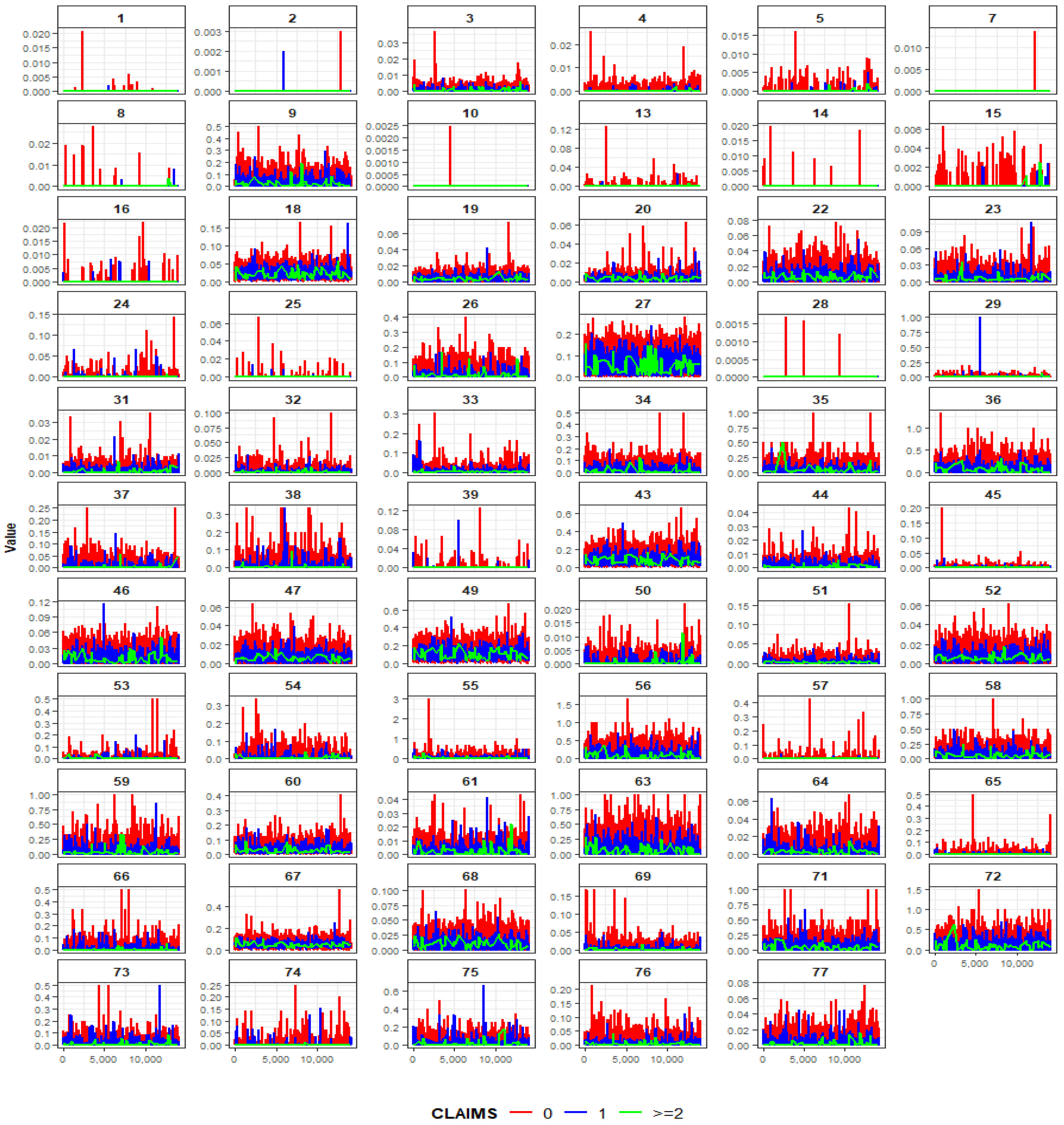
Appendix D. Visualisation of Driver Variables
Appendix D.1. Driving Variables by Claim Frequency
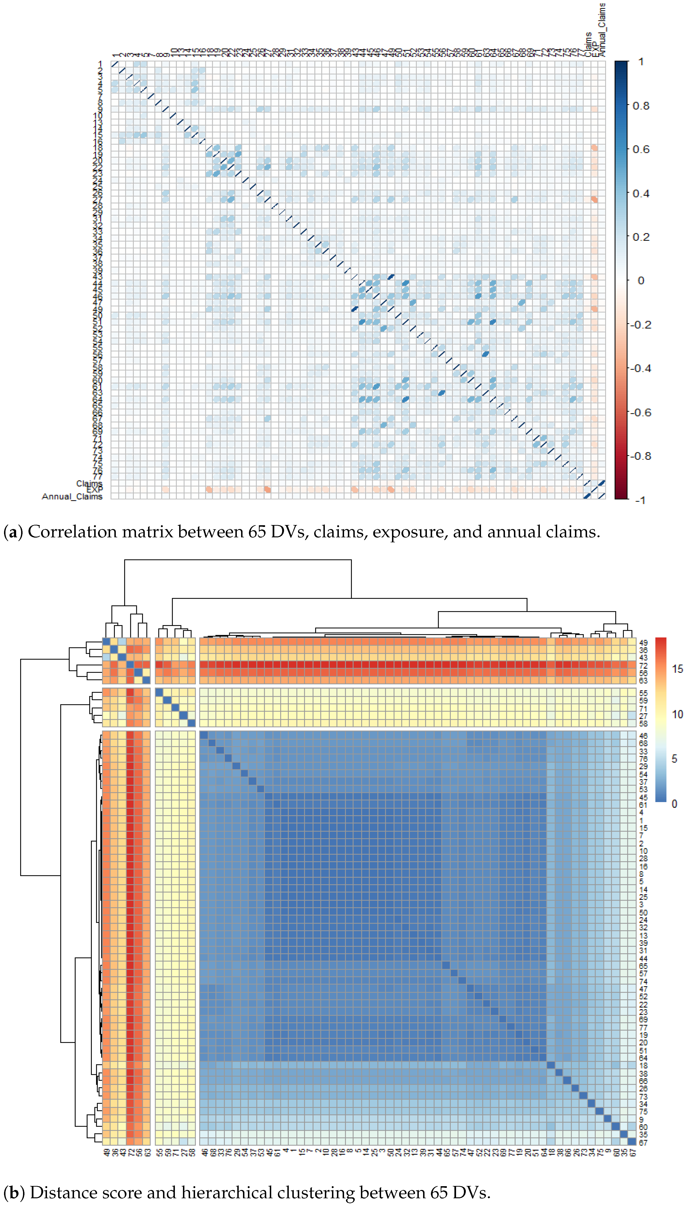
Appendix D.2. Correlation Matrix and Hierarchical Clustering of Driving Variables
Appendix E. Parameter Estimates of All Models
| TPL-1 | |||||||||||||||||
| glmnet with 100 Repeats | glm | glmnet with 100 Repeats | glm | glmnet with 100 Repeats | glm | ||||||||||||
| Measures | MSE | MAE | Deviance | Poisson | Measures | MSE | MAE | Deviance | Poisson | Measures | MSE | MAE | Deviance | Poisson | |||
| DVs | DVs | DVs | |||||||||||||||
| 1 | - | 34 | 7 | −0.0029 | - | 28 | 3 | 126 | 61 | −0.0031 | - | 55 | - | 119 | 68 | 0.0082 | 0.0134 |
| 2 | 89 | 232 | 228 | 0.0176 | 0.0159 | 29 | 227 | 276 | 279 | 0.0279 | 0.0360 | 56 | 37 | 136 | 123 | 0.0149 | 0.0061 |
| 3 | 180 | 317 | 337 | 0.0402 | 0.0619 | 31 | 251 | 324 | 337 | 0.0409 | 0.0535 | 57 | 139 | 310 | 334 | −0.0446 | −0.1696 |
| 4 | 140 | 307 | 334 | −0.0409 | −0.0987 | 32 | 302 | 327 | 341 | 0.0474 | 0.0513 | 58 | 24 | 147 | 109 | 0.0115 | 0.0095 |
| 5 | 3 | 109 | 61 | 0.0085 | - | 33 | 133 | 273 | 266 | 0.0256 | 0.0393 | 59 | 68 | 252 | 229 | 0.0282 | 0.0448 |
| 7 | - | 136 | 116 | −0.0021 | −0.0830 | 34 | - | 85 | 20 | −0.0073 | - | 60 | 95 | 198 | 191 | −0.0243 | −0.0091 |
| 8 | 7 | 95 | 37 | −0.0011 | - | 35 | 146 | 245 | 242 | 0.0222 | 0.0168 | 61 | 255 | 317 | 320 | 0.0426 | 0.0626 |
| 9 | 272 | 310 | 320 | 0.0417 | 0.0546 | 36 | 262 | 320 | 334 | 0.0576 | 0.0797 | 63 | 98 | 242 | 235 | 0.0219 | 0.0346 |
| 10 | - | 17 | - | - | - | 37 | 292 | 327 | 334 | 0.0424 | 0.0518 | 64 | 30 | 194 | 160 | −0.0264 | −0.0348 |
| 13 | 10 | 140 | 72 | −0.0154 | −0.0253 | 38 | 184 | 290 | 289 | 0.0238 | 0.0263 | 65 | - | 99 | 41 | −0.0084 | - |
| 14 | - | 105 | 14 | −0.0031 | - | 39 | 71 | 232 | 228 | 0.0122 | 0.0160 | 66 | 41 | 164 | 133 | 0.0164 | 0.0173 |
| 15 | 14 | 119 | 68 | −0.0190 | −0.0065 | 43 | 78 | 204 | 204 | −0.0381 | −0.0505 | 67 | 329 | 330 | 341 | −0.1400 | −0.1706 |
| 16 | 3 | 113 | 65 | 0.0001 | −0.0004 | 44 | 3 | 112 | 41 | −0.0113 | - | 68 | 17 | 102 | 61 | −0.0135 | - |
| 18 | 316 | 327 | 341 | 0.0969 | 0.1254 | 45 | 3 | 78 | 48 | 0.0172 | - | 69 | 17 | 188 | 140 | −0.0166 | −0.0320 |
| 19 | - | 85 | 20 | 0.0021 | - | 46 | 31 | 194 | 164 | 0.0210 | 0.0361 | 71 | 78 | 231 | 224 | 0.0172 | 0.0185 |
| 20 | 173 | 310 | 323 | 0.0363 | 0.0563 | 47 | 177 | 314 | 330 | −0.0611 | −0.0918 | 72 | 187 | 303 | 297 | 0.0319 | 0.0418 |
| 22 | 41 | 205 | 177 | 0.0133 | 0.0309 | 49 | 95 | 245 | 252 | −0.0341 | −0.0448 | 73 | 302 | 327 | 341 | 0.0587 | 0.0743 |
| 23 | - | 133 | 75 | −0.0051 | −0.0235 | 50 | 72 | 228 | 218 | 0.0157 | 0.0205 | 74 | 102 | 242 | 242 | 0.0216 | 0.0350 |
| 24 | 136 | 272 | 262 | 0.0213 | 0.0236 | 51 | 116 | 289 | 306 | −0.0517 | −0.0944 | 75 | 336 | 330 | 341 | 0.0621 | 0.0659 |
| 25 | - | 119 | 58 | −0.0087 | - | 52 | 150 | 307 | 324 | −0.0397 | −0.0623 | 76 | 48 | 239 | 235 | −0.0236 | −0.0565 |
| 26 | 58 | 160 | 139 | 0.0129 | 0.0024 | 53 | 65 | 174 | 157 | 0.0156 | 0.0107 | 77 | 157 | 307 | 324 | 0.0324 | 0.0549 |
| 27 | 17 | 160 | 129 | −0.0205 | −0.0402 | 54 | 163 | 262 | 272 | 0.0209 | 0.0208 | ||||||
| TPA-1 | |||||||||||||||||
| glmnet with 100 Repeats | glm | glmnet with 100 Repeats | glm | glmnet with 100 Repeats | glm | ||||||||||||
| Measures | MSE | MAE | Deviance | Poisson | Measures | MSE | MAE | Deviance | Poisson | Measures | MSE | MAE | Deviance | Poisson | |||
| DVs | DVs | DVs | |||||||||||||||
| 1 | 3 | 41 | 24 | −0.0712 | - | 28 | - | 79 | - | - | - | 55 | - | 41 | 20 | 0.0030 | - |
| 2 | 61 | 95 | 68 | 0.0360 | 0.0149 | 29 | 228 | 279 | 276 | 0.0311 | 0.0357 | 56 | 14 | 99 | 61 | 0.0311 | - |
| 3 | 160 | 317 | 310 | 0.0512 | 0.0608 | 31 | 217 | 316 | 313 | 0.0514 | 0.0536 | 57 | 78 | 306 | 327 | −0.0797 | −0.1726 |
| 4 | 89 | 296 | 310 | −0.0630 | −0.1035 | 32 | 319 | 337 | 340 | 0.0552 | 0.0503 | 58 | - | 38 | 3 | 0.0297 | - |
| 5 | - | 61 | 10 | 0.0482 | - | 33 | 78 | 248 | 214 | 0.0352 | 0.0363 | 59 | 31 | 204 | 139 | 0.0374 | 0.0478 |
| 7 | - | 24 | - | - | - | 34 | - | 38 | 17 | −0.0201 | - | 60 | 58 | 143 | 126 | −0.0288 | −0.0093 |
| 8 | - | 34 | 13 | −0.0067 | - | 35 | 102 | 190 | 177 | 0.0258 | 0.0199 | 61 | 163 | 283 | 282 | 0.0595 | 0.0702 |
| 9 | 187 | 300 | 289 | 0.0517 | 0.0579 | 36 | 248 | 334 | 330 | 0.0703 | 0.0775 | 63 | 41 | 194 | 150 | 0.0358 | 0.0422 |
| 10 | - | - | - | - | - | 37 | 285 | 334 | 330 | 0.0513 | 0.0530 | 64 | 27 | 143 | 89 | −0.0551 | −0.0317 |
| 13 | - | 48 | 20 | −0.0144 | - | 38 | 160 | 231 | 218 | 0.0298 | 0.0271 | 65 | - | 17 | 10 | −0.0100 | - |
| 14 | - | 62 | - | - | - | 39 | 7 | 116 | 71 | 0.0132 | 0.0163 | 66 | 17 | 109 | 55 | 0.0221 | - |
| 15 | 3 | 86 | 31 | −0.0200 | - | 43 | 48 | 235 | 204 | −0.0577 | −0.0510 | 67 | 336 | 340 | 340 | −0.1752 | −0.1686 |
| 16 | - | 14 | 3 | −0.0088 | - | 44 | - | 44 | 7 | −0.0294 | - | 68 | - | 85 | 55 | −0.0201 | - |
| 18 | 333 | 340 | 340 | 0.1212 | 0.1205 | 45 | 3 | 72 | 44 | 0.0293 | - | 69 | 7 | 99 | 34 | −0.0334 | - |
| 19 | 10 | 65 | 17 | 0.0146 | - | 46 | 10 | 130 | 51 | 0.0410 | - | 71 | 37 | 129 | 102 | 0.0291 | 0.0204 |
| 20 | 112 | 286 | 272 | 0.0426 | 0.0567 | 47 | 170 | 327 | 327 | −0.0773 | −0.0913 | 72 | 156 | 269 | 248 | 0.0479 | 0.0443 |
| 22 | 20 | 143 | 85 | 0.0300 | 0.0282 | 49 | 58 | 194 | 187 | −0.0470 | −0.0367 | 73 | 289 | 340 | 337 | 0.0710 | 0.0733 |
| 23 | - | 55 | 14 | −0.0171 | - | 50 | 27 | 129 | 92 | 0.0259 | 0.0206 | 74 | 51 | 228 | 167 | 0.0301 | 0.0341 |
| 24 | 58 | 188 | 147 | 0.0237 | 0.0230 | 51 | 51 | 282 | 262 | −0.0718 | −0.0918 | 75 | 316 | 340 | 333 | 0.0748 | 0.0709 |
| 25 | - | 34 | 3 | −0.0843 | - | 52 | 136 | 306 | 303 | −0.0493 | −0.0618 | 76 | 41 | 225 | 184 | −0.0446 | −0.0565 |
| 26 | 21 | 68 | 38 | 0.0201 | - | 53 | 10 | 71 | 54 | 0.0182 | - | 77 | 116 | 290 | 273 | 0.0457 | 0.0554 |
| 27 | 10 | 153 | 105 | −0.0349 | −0.0359 | 54 | 109 | 176 | 183 | 0.0259 | 0.0256 | ||||||
| : TPLA-2 | : TPLA-2 | : TPLN-2 | : TPLN-2 | ||||||||||||||||||||
|---|---|---|---|---|---|---|---|---|---|---|---|---|---|---|---|---|---|---|---|---|---|---|---|
| Groups | Low | High | Low | High | Low | High | Low | High | |||||||||||||||
| 0.70 | 0.30 | 0.79 | 0.21 | 0.85 | 0.15 | 0.90 | 0.10 | ||||||||||||||||
| 43 | 19 | 49 | 13 | 53 | 9 | 56 | 6 | ||||||||||||||||
| 17 | 22 | 38 | 14 | 42 | 23 | 43 | 28 | ||||||||||||||||
| DVs | DVs | DVs | DVs | DVs | DVs | DVs | DVs | ||||||||||||||||
| 2 | - | - | 2 | 42 | 0.0277 | 2 | - | - | 2 | 19 | 0.0169 | 2 | - | - | 2 | 18 | 0.0108 | 2 | - | - | 2 | 5 | 0.0250 |
| 3 | 8 | 0.0093 | 3 | 31 | 0.0356 | 3 | 52 | 0.0331 | 3 | - | - | 3 | 116 | 0.0515 | 3 | 5 | 0.0235 | 3 | 118 | 0.0403 | 3 | - | - |
| 4 | 49 | −0.0567 | 4 | 42 | 0.0366 | 4 | 254 | −0.0714 | 4 | 43 | 0.0466 | 4 | 356 | −0.0748 | 4 | 76 | 0.0864 | 4 | 357 | −0.0833 | 4 | 129 | 0.1443 |
| 7 | - | - | 7 | - | - | 7 | - | - | 7 | - | - | 7 | - | - | 7 | - | - | 7 | - | - | 7 | - | - |
| 9 | 95 | 0.0636 | 9 | 3 | −0.0081 | 9 | 350 | 0.0976 | 9 | 3 | −0.0416 | 9 | 348 | 0.0953 | 9 | 10 | −0.0421 | 9 | 357 | 0.0859 | 9 | 15 | −0.0528 |
| 13 | 4 | −0.0882 | 13 | 48 | 0.0410 | 13 | 66 | −0.0648 | 13 | 87 | 0.0824 | 13 | 243 | −0.0513 | 13 | 91 | 0.0814 | 13 | 278 | −0.0545 | 13 | 83 | 0.0667 |
| 15 | 11 | −0.0010 | 15 | 6 | −0.0205 | 15 | 26 | −0.0193 | 15 | - | - | 15 | 44 | −0.0643 | 15 | - | - | 15 | 22 | −0.0286 | 15 | 8 | 0.0355 |
| 16 | 11 | −0.0584 | 16 | 17 | 0.0252 | 16 | 33 | −0.0353 | 16 | 68 | 0.0424 | 16 | 22 | −0.0077 | 16 | 55 | 0.0426 | 16 | 11 | −0.0097 | 16 | 15 | 0.0219 |
| 18 | 46 | 0.0820 | 18 | 36 | 0.0608 | 18 | 210 | 0.0827 | 18 | 3 | 0.0867 | 18 | 323 | 0.0764 | 18 | - | - | 18 | 343 | 0.1031 | 18 | - | - |
| 20 | 15 | −0.0056 | 20 | 45 | 0.0351 | 20 | 40 | 0.0428 | 20 | - | - | 20 | 207 | 0.0437 | 20 | - | - | 20 | 171 | 0.0363 | 20 | 3 | 0.0768 |
| 22 | 72 | −0.0633 | 22 | 89 | 0.0407 | 22 | 15 | −0.0469 | 22 | 8 | 0.0272 | 22 | 36 | −0.0138 | 22 | 5 | 0.0174 | 22 | 47 | −0.0218 | 22 | 18 | 0.0432 |
| 23 | 11 | 0.0060 | 23 | 6 | 0.0196 | 23 | 33 | 0.0084 | 23 | 3 | −0.0091 | 23 | 101 | 0.0292 | 23 | 8 | −0.0442 | 23 | 139 | 0.0280 | 23 | 40 | −0.0761 |
| 24 | 35 | 0.0645 | 24 | 11 | 0.0316 | 24 | 195 | 0.0727 | 24 | 3 | 0.0456 | 24 | 348 | 0.0904 | 24 | - | - | 24 | 339 | 0.0844 | 24 | - | - |
| 26 | 113 | 0.0577 | 26 | 6 | −0.0608 | 26 | 199 | 0.0516 | 26 | 11 | −0.0282 | 26 | 185 | 0.0377 | 26 | 3 | −0.0094 | 26 | 154 | 0.0270 | 26 | 8 | −0.0363 |
| 27 | 61 | −0.0502 | 27 | 34 | 0.0476 | 27 | 95 | −0.0422 | 27 | 5 | −0.0264 | 27 | 214 | −0.0478 | 27 | 10 | −0.0320 | 27 | 75 | −0.0287 | 27 | 33 | −0.0863 |
| 29 | 12 | −0.0749 | 29 | 95 | 0.0211 | 29 | 48 | −0.0497 | 29 | 32 | 0.0179 | 29 | 163 | 0.0476 | 29 | 11 | −0.0494 | 29 | 157 | 0.0358 | 29 | 13 | 0.0148 |
| 31 | 12 | 0.0563 | 31 | 17 | 0.0219 | 31 | 74 | 0.0495 | 31 | 3 | 0.0463 | 31 | 287 | 0.0555 | 31 | 5 | 0.0323 | 31 | 286 | 0.0549 | 31 | - | - |
| 32 | 46 | 0.0614 | 32 | 61 | 0.0320 | 32 | 332 | 0.1115 | 32 | - | - | 32 | 345 | 0.0893 | 33 | 8 | −0.0312 | 32 | 332 | 0.0801 | 32 | - | - |
| 33 | 23 | 0.0492 | 33 | - | - | 33 | 147 | 0.0523 | 33 | - | - | 33 | 309 | 0.0569 | 33 | - | - | 33 | 264 | 0.0492 | 33 | 5 | −0.0615 |
| 35 | - | - | 35 | 25 | 0.0343 | 35 | 85 | 0.0277 | 35 | - | - | 35 | 127 | 0.0265 | 35 | - | - | 35 | 61 | 0.0227 | 35 | 5 | 0.0954 |
| 36 | 69 | 0.0575 | 36 | 3 | 0.0776 | 36 | 137 | 0.0411 | 36 | - | - | 36 | 264 | 0.0536 | 36 | - | - | 36 | 318 | 0.0591 | 36 | 3 | −0.0304 |
| 37 | 243 | 0.1047 | 37 | 14 | 0.0276 | 37 | 354 | 0.1337 | 37 | - | - | 37 | 355 | 0.1239 | 37 | - | - | 37 | 357 | 0.1153 | 37 | - | - |
| 38 | 38 | −0.0502 | 38 | 22 | 0.0304 | 38 | 78 | −0.0596 | 38 | 16 | 0.0401 | 38 | 127 | −0.0437 | 38 | 39 | 0.0386 | 38 | 25 | −0.0237 | 38 | 18 | 0.0239 |
| 39 | 87 | −0.0652 | 39 | - | - | 39 | 251 | −0.0819 | 39 | - | - | 39 | 327 | −0.1015 | 39 | 3 | 0.0148 | 39 | 132 | −0.1482 | 39 | - | - |
| 43 | 27 | −0.0380 | 43 | 6 | 0.0150 | 43 | 59 | −0.0501 | 43 | 13 | −0.0375 | 43 | 65 | −0.0265 | 43 | 26 | −0.0868 | 43 | 82 | −0.0289 | 43 | 83 | −0.0808 |
| 46 | 4 | −0.0310 | 46 | 67 | 0.0310 | 46 | 15 | 0.0088 | 46 | 5 | 0.0376 | 46 | 26 | 0.0188 | 46 | - | - | 46 | 36 | 0.0345 | 46 | 10 | 0.0868 |
| 47 | 60 | −0.0564 | 47 | 6 | −0.0103 | 47 | 225 | −0.0711 | 47 | 3 | −0.0745 | 47 | 341 | −0.0804 | 47 | - | - | 47 | 321 | −0.0713 | 47 | - | - |
| 49 | 15 | −0.0375 | 49 | - | - | 49 | 59 | −0.0326 | 49 | 11 | −0.0564 | 49 | 54 | −0.0219 | 49 | 75 | −0.0759 | 49 | 193 | −0.0381 | 49 | 26 | −0.0744 |
| 50 | 15 | −0.0394 | 50 | 11 | 0.0320 | 50 | 29 | −0.0543 | 50 | - | - | 50 | 87 | −0.0308 | 50 | 13 | 0.0291 | 50 | 64 | −0.0244 | 50 | 22 | 0.0360 |
| 51 | 152 | −0.0853 | 51 | 150 | 0.0625 | 51 | 206 | −0.0769 | 51 | 8 | 0.0623 | 51 | 214 | −0.0555 | 51 | - | - | 51 | 314 | −0.0776 | 51 | 7 | 0.0969 |
| 52 | 4 | −0.0013 | 52 | 45 | −0.0826 | 52 | 151 | −0.0387 | 52 | 8 | −0.0763 | 52 | 268 | −0.0416 | 52 | 16 | −0.0202 | 52 | 293 | −0.0462 | 52 | 7 | −0.0014 |
| 53 | 152 | 0.0733 | 53 | - | - | 53 | 95 | 0.0407 | 53 | 3 | 0.0167 | 53 | 51 | −0.0297 | 53 | 10 | 0.0507 | 53 | 110 | 0.0380 | 53 | 5 | 0.0094 |
| 54 | 34 | 0.0424 | 54 | 6 | 0.0210 | 54 | 56 | 0.0202 | 54 | 3 | 0.0047 | 54 | 47 | 0.0256 | 54 | 3 | 0.0332 | 54 | 232 | 0.0392 | 54 | - | - |
| 55 | 11 | 0.0340 | 55 | - | - | 55 | 158 | 0.0483 | 55 | 16 | −0.0460 | 55 | 152 | 0.0354 | 55 | 13 | −0.0540 | 55 | 228 | 0.0491 | 55 | 33 | −0.1115 |
| 56 | 49 | 0.0443 | 56 | 3 | −0.0516 | 56 | 122 | 0.0412 | 56 | 3 | −0.0275 | 56 | 196 | 0.0327 | 56 | 13 | −0.0398 | 56 | 132 | 0.0401 | 56 | 20 | −0.0636 |
| 57 | 15 | −0.0626 | 57 | - | - | 57 | 214 | −0.0672 | 57 | 92 | 0.0740 | 57 | 337 | −0.0673 | 57 | 49 | −0.1974 | 57 | 346 | −0.0739 | 57 | 45 | −0.2011 |
| 58 | 49 | 0.0432 | 58 | 78 | −0.0545 | 58 | 74 | 0.0290 | 58 | 57 | −0.0548 | 58 | 91 | 0.0349 | 58 | 96 | −0.0789 | 58 | 100 | 0.0280 | 58 | 98 | −0.0941 |
| 59 | 65 | 0.0571 | 59 | - | - | 59 | 207 | 0.0566 | 59 | 33 | −0.0480 | 59 | 294 | 0.0557 | 59 | 91 | −0.0799 | 59 | 285 | 0.0552 | 59 | 50 | −0.0947 |
| 60 | 50 | −0.0413 | 60 | 8 | 0.0345 | 60 | 55 | −0.0442 | 60 | - | - | 60 | 239 | −0.0514 | 60 | 10 | 0.0615 | 60 | 221 | −0.0514 | 60 | 10 | 0.0957 |
| 61 | 8 | 0.0465 | 61 | 31 | 0.0258 | 61 | 26 | 0.0135 | 61 | 32 | 0.0445 | 61 | 149 | 0.0485 | 61 | - | - | 61 | 146 | 0.0504 | 61 | 8 | 0.0182 |
| 63 | 8 | −0.0378 | 63 | 67 | 0.0422 | 63 | 4 | −0.0054 | 63 | - | - | 63 | 15 | −0.0068 | 63 | 16 | 0.0675 | 63 | 50 | 0.0219 | 63 | 3 | 0.0811 |
| 64 | 26 | −0.0629 | 64 | - | - | 64 | 88 | −0.0593 | 64 | - | - | 64 | 142 | −0.0489 | 64 | - | - | 64 | 211 | −0.0458 | 64 | 35 | 0.0833 |
| 66 | 38 | 0.0499 | 66 | - | - | 66 | 225 | 0.0496 | 66 | - | - | 66 | 254 | 0.0416 | 66 | - | - | 66 | 211 | 0.0400 | 66 | 3 | −0.0610 |
| 67 | 31 | −0.0420 | 67 | 176 | −0.1401 | 67 | 310 | −0.0912 | 67 | 187 | −0.1461 | 67 | 363 | −0.1275 | 67 | 112 | −0.0977 | 67 | 357 | −0.1418 | 67 | 97 | −0.1485 |
| 69 | 19 | −0.0407 | 69 | 76 | 0.0508 | 69 | 121 | −0.0523 | 69 | - | - | 69 | 98 | −0.0353 | 69 | - | - | 69 | 46 | −0.0232 | 69 | 5 | −0.0503 |
| 71 | 30 | 0.0396 | 71 | 6 | −0.0682 | 71 | 192 | 0.0464 | 71 | 8 | −0.0405 | 71 | 175 | 0.0328 | 71 | 3 | −0.0374 | 71 | 100 | 0.0228 | 71 | 2 | −0.0005 |
| 72 | 8 | 0.0326 | 72 | 11 | 0.0267 | 72 | 41 | 0.0265 | 72 | - | - | 72 | 76 | 0.0236 | 72 | - | - | 72 | 104 | 0.0219 | 72 | 10 | 0.0867 |
| 73 | 42 | 0.0594 | 73 | 50 | 0.0344 | 73 | 185 | 0.0747 | 73 | 5 | 0.0291 | 73 | 268 | 0.0709 | 73 | 5 | 0.0354 | 73 | 321 | 0.0709 | 73 | 2 | 0.0015 |
| 74 | - | - | 74 | 17 | 0.0248 | 74 | 122 | 0.0458 | 74 | 3 | 0.0242 | 74 | 276 | 0.0611 | 74 | - | - | 74 | 188 | 0.0446 | 74 | - | - |
| 75 | 15 | 0.0488 | 75 | 107 | 0.0456 | 75 | 254 | 0.0707 | 75 | 16 | 0.0436 | 75 | 301 | 0.0730 | 75 | 3 | 0.0451 | 75 | 332 | 0.0844 | 75 | - | - |
| 76 | 27 | −0.0662 | 76 | 6 | −0.0343 | 76 | 151 | −0.0588 | 76 | 5 | −0.0035 | 76 | 276 | −0.0549 | 76 | 10 | 0.0779 | 76 | 271 | −0.0491 | 76 | 27 | 0.0867 |
| 77 | 7 | 0.0400 | 77 | 14 | 0.0209 | 77 | 26 | 0.0373 | 77 | 5 | 0.0330 | 77 | 36 | 0.0075 | 77 | 24 | 0.0574 | 77 | 100 | 0.0391 | 77 | 5 | 0.0448 |
| PML | PMA | ZIPA | ||||||||||||||
|---|---|---|---|---|---|---|---|---|---|---|---|---|---|---|---|---|
| 43 | 19 | 45 | 17 | 62 | 62 | |||||||||||
| 45 | 18 | 39 | 40 | 4 | 45 | |||||||||||
| DVs | Low | High | DVs | Low | High | DVs | Zero | Count | ||||||||
| 3 | 118 | 0.0182 | 47 | 0.0983 | 3 | 71 | 0.0380 | 126 | 0.1182 | 3 | 44 | −0.0022 | - | 291 | 0.0404 | 0.0514 |
| 9 | 88 | −0.0003 | 20 | 0.0275 | 9 | 27 | −0.0226 | 16 | 0.0106 | 9 | 20 | −0.0047 | - | 172 | 0.0170 | 0.0450 |
| 18 | 324 | 0.0636 | 27 | 0.0477 | 18 | 206 | 0.0877 | 149 | 0.1078 | 18 | - | - | - | 88 | 0.0044 | 0.1352 |
| 19 | 311 | 0.0491 | 3 | 0.1058 | 19 | 200 | 0.0877 | 82 | 0.0821 | 19 | 10 | −0.0003 | - | 136 | 0.0050 | −0.0263 |
| 20 | 78 | −0.0197 | 37 | 0.0919 | 20 | 71 | −0.0443 | 27 | −0.0532 | 20 | 34 | −0.0053 | - | 291 | 0.0552 | 0.0717 |
| 22 | 162 | 0.0098 | 54 | 0.0633 | 22 | 91 | −0.0484 | 101 | 0.0839 | 22 | 47 | −0.0104 | - | 217 | 0.0333 | 0.0441 |
| 23 | 335 | −0.2076 | 24 | −0.2634 | 23 | 219 | −0.2801 | 159 | −0.2732 | 23 | - | - | - | 84 | −0.0025 | −0.0247 |
| 26 | 250 | 0.0259 | 98 | 0.0370 | 26 | 212 | 0.0375 | 81 | 0.0119 | 26 | 3 | 1.91 × 10⁻⁵ | - | 125 | 0.0069 | 0.0014 |
| 27 | 338 | 0.0450 | 3 | 0.0068 | 27 | 251 | 0.0755 | 60 | 0.0576 | 27 | 10 | 0.0004 | - | 339 | −0.1900 | −0.0495 |
| 29 | 324 | 0.0355 | 17 | 0.0633 | 29 | 172 | 0.0663 | 79 | 0.0722 | 29 | 24 | −0.0005 | - | 267 | 0.0182 | 0.0363 |
| 31 | 294 | 0.0352 | 14 | 0.0390 | 31 | 165 | 0.0637 | 87 | 0.0496 | 31 | 20 | −0.0024 | - | 234 | 0.0265 | 0.0515 |
| 33 | 138 | −0.0150 | - | - | 33 | 50 | −0.0516 | 13 | −0.0265 | 33 | 55 | −0.0123 | - | 213 | 0.0243 | 0.0426 |
| 34 | 287 | 0.0369 | 7 | 0.1254 | 34 | 127 | 0.0586 | 57 | 0.0533 | 34 | 3 | −0.0001 | - | 88 | −0.0022 | −0.0234 |
| 35 | 331 | 0.0578 | 7 | 0.0130 | 35 | 299 | 0.1089 | 43 | 0.0735 | 35 | 20 | −0.0029 | - | 132 | 0.0099 | 0.0232 |
| 36 | 335 | 0.0501 | 31 | 0.0450 | 36 | 214 | 0.0690 | 120 | 0.0642 | 36 | 30 | −0.0103 | - | 281 | 0.0464 | 0.0752 |
| 37 | 304 | 0.0284 | 13 | 0.0522 | 37 | 183 | 0.0416 | 51 | 0.0567 | 37 | 10 | −0.0009 | - | 298 | 0.0429 | 0.0524 |
| 38 | 230 | −0.0516 | 7 | 0.0002 | 38 | 121 | −0.1553 | 40 | 0.0017 | 38 | 98 | −0.0265 | -39.0618 | 121 | 0.0076 | −0.0065 |
| 43 | 88 | −0.0267 | 3 | −0.0238 | 43 | 36 | −0.0296 | 44 | −0.0703 | 43 | 17 | 0.0008 | - | 173 | −0.0397 | −0.0471 |
| 44 | 57 | 0.0078 | - | - | 44 | 54 | 0.0575 | 37 | 0.0932 | 44 | - | - | - | 155 | −0.0099 | −0.0287 |
| 45 | 274 | 0.0541 | 24 | 0.0395 | 45 | 249 | 0.1177 | 79 | 0.0982 | 45 | 10 | −0.0005 | - | 153 | 0.0090 | 0.0188 |
| 46 | 338 | −0.0957 | 14 | −0.0442 | 46 | 259 | −0.1665 | 78 | −0.1081 | 46 | 30 | −0.0042 | - | 264 | 0.0569 | 0.0362 |
| 47 | 338 | −0.1644 | 20 | −0.0469 | 47 | 292 | −0.2914 | 77 | −0.1493 | 47 | 3 | 0.0000 | - | 322 | −0.0843 | −0.0940 |
| 49 | 249 | 0.0241 | 10 | 0.0235 | 49 | 91 | 0.0430 | 23 | 0.0378 | 49 | 165 | 0.0366 | −0.0193 | 251 | −0.1070 | −0.0597 |
| 50 | 331 | −0.0898 | 24 | −0.0447 | 50 | 197 | −0.1691 | 126 | −0.1419 | 50 | - | - | - | 122 | 0.0077 | 0.0145 |
| 51 | 335 | −0.0981 | 14 | −0.0381 | 51 | 225 | −0.1602 | 119 | −0.1378 | 51 | 17 | 0.0004 | - | 301 | −0.0865 | −0.0868 |
| 52 | 314 | 0.0265 | 37 | 0.0265 | 52 | 93 | 0.0447 | 81 | 0.0538 | 52 | 10 | 0.0023 | - | 311 | −0.0738 | −0.0660 |
| 54 | 84 | 0.0134 | - | - | 54 | 40 | 0.0111 | 7 | 0.0496 | 54 | 17 | −0.0013 | - | 213 | 0.0197 | 0.0182 |
| 55 | 112 | 0.0183 | 7 | 0.0196 | 55 | 33 | 0.0027 | 14 | −0.0053 | 55 | 7 | 0.0001 | - | 88 | 0.0016 | 0.0109 |
| 56 | 142 | 0.0193 | 44 | 0.0636 | 56 | 33 | 0.0478 | 114 | 0.0780 | 56 | 3 | −0.0003 | - | 75 | 0.0012 | 0.0002 |
| 58 | 240 | 0.0298 | 17 | 0.0632 | 58 | 154 | 0.0718 | 62 | 0.0692 | 58 | 3 | −0.0001 | - | 128 | 0.0087 | 0.0157 |
| 59 | 294 | −0.0433 | 17 | −0.0817 | 59 | 115 | −0.1431 | 73 | −0.1543 | 59 | 24 | −0.0035 | - | 200 | 0.0189 | 0.0409 |
| 60 | 318 | 0.0574 | 24 | 0.0934 | 60 | 183 | 0.1142 | 162 | 0.0945 | 60 | 13 | 0.0024 | - | 231 | −0.0259 | −0.0053 |
| 61 | 223 | 0.0297 | 3 | 0.0193 | 61 | 167 | 0.0773 | 37 | 0.0514 | 61 | 20 | −0.0032 | - | 244 | 0.0403 | 0.0560 |
| 63 | 189 | −0.0652 | 20 | −0.0031 | 63 | 162 | −0.1524 | 125 | −0.0583 | 63 | 37 | −0.0057 | - | 98 | 0.0088 | 0.0362 |
| 64 | 162 | 0.0132 | 7 | 0.0346 | 64 | 71 | 0.0231 | 7 | 0.0641 | 64 | - | - | - | 139 | −0.0220 | −0.0409 |
| 66 | 338 | −0.1689 | 7 | −0.0538 | 66 | 297 | −0.3054 | 64 | −0.1943 | 66 | 7 | −0.0001 | - | 81 | 0.0050 | 0.0175 |
| 67 | 88 | −0.0263 | - | - | 67 | 37 | −0.0730 | 40 | 0.0416 | 67 | 20 | 0.0044 | - | 339 | −0.1312 | −0.1510 |
| 68 | 210 | −0.0265 | 7 | −0.0102 | 68 | 90 | −0.0940 | 52 | −0.1397 | 68 | 7 | 0.0001 | - | 67 | −0.0013 | −0.0041 |
| 69 | 199 | 0.0210 | 17 | 0.0611 | 69 | 95 | 0.0537 | 26 | 0.0420 | 69 | 7 | 0.0005 | - | 180 | −0.0190 | −0.0286 |
| 71 | 270 | 0.0388 | 14 | 0.0725 | 71 | 141 | 0.0869 | 76 | 0.0686 | 71 | 34 | −0.0040 | - | 145 | 0.0098 | 0.0114 |
| 72 | 318 | 0.0473 | 183 | 0.1172 | 72 | 217 | 0.0774 | 194 | 0.0950 | 72 | 30 | −0.0040 | - | 268 | 0.0338 | 0.0391 |
| 73 | 335 | 0.0631 | 88 | 0.1193 | 73 | 242 | 0.1072 | 109 | 0.1064 | 73 | 75 | −0.0129 | −0.1323 | 288 | 0.0391 | 0.0617 |
| 75 | 321 | −0.0545 | 27 | −0.0622 | 75 | 142 | −0.1177 | 136 | −0.1645 | 75 | 20 | −0.0022 | - | 301 | 0.0511 | 0.0634 |
| 76 | 257 | 0.0361 | 10 | 0.0327 | 76 | 161 | 0.0722 | 83 | 0.0827 | 76 | 7 | 0.0009 | - | 244 | −0.0380 | −0.0656 |
| 77 | 284 | 0.0324 | 17 | 0.0370 | 77 | 170 | 0.0740 | 74 | 0.0615 | 77 | 98 | −0.0189 | −34.9726 | 149 | 0.0132 | −0.0313 |
References
- Ayuso, Mercedes, Montserrat Guillen, and Jens Perch Nielsen. 2019. Improving automobile insurance ratemaking using telematics: Incorporating mileage and driver behaviour data. Transportation 46: 735–52. [Google Scholar] [CrossRef]
- Banerjee, Prithish, Broti Garai, Himel Mallick, Shrabanti Chowdhury, and Saptarshi Chatterjee. 2018. A note on the adaptive lasso for zero-inflated Poisson regression. Journal of Probability and Statistics 2018: 2834183. [Google Scholar] [CrossRef]
- Barry, Laurence, and Arthur Charpentier. 2020. Personalization as a promise: Can big data change the practice of insurance? Big Data & Society 7: 2053951720935143. [Google Scholar]
- Bhattacharya, Sakyajit, and Paul D. McNicholas. 2014. An adaptive lasso-penalized BIC. arXiv arXiv:1406.1332. [Google Scholar]
- Bolderdijk, Jan Willem, Jasper Knockaert, E. M. Steg, and Erik T. Verhoef. 2011. Effects of Pay-As-You-Drive vehicle insurance on young drivers’ speed choice: Results of a dutch field experiment. Accident Analysis & Prevention 43: 1181–86. [Google Scholar]
- Cameron, A. Colin, and Pravin K. Trivedi. 1990. Regression-based tests for overdispersion in the Poisson model. Journal of Econometrics 46: 347–64. [Google Scholar] [CrossRef]
- Chan, Jennifer S. K., S. T. Boris Choy, Udi Makov, Ariel Shamir, and Vered Shapovalov. 2022. Variable selection algorithm for a mixture of poisson regression for handling overdispersion in claims frequency modeling using telematics car driving data. Risks 10: 83. [Google Scholar] [CrossRef]
- Chassagnon, Arnold, and Pierre-André Chiappori. 1997. Insurance under Moral Hazard and Adverse Selection: The Case of Pure Competition. Delta-CREST Document. Available online: https://econpapers.repec.org/paper/fthlavale/28.htm (accessed on 1 August 2024).
- Czado, Claudia, Tilmann Gneiting, and Leonhard Held. 2009. Predictive model assessment for count data. Biometrics 65: 1254–61. [Google Scholar] [CrossRef]
- Dean, Curtis Gary. 1997. An introduction to credibility. In Casualty Actuary Forum. Arlington: Casualty Actuarial Society, pp. 55–66. Available online: https://www.casact.org/sites/default/files/database/forum_97wforum_97wf055.pdf (accessed on 1 August 2024).
- Deng, Min, Mostafa S. Aminzadeh, and Banghee So. 2024. Inference for the parameters of a zero-inflated poisson predictive model. Risks 12: 104. [Google Scholar] [CrossRef]
- Duval, Francis, Jean-Philippe Boucher, and Mathieu Pigeon. 2023. Enhancing claim classification with feature extraction from anomaly-detection-derived routine and peculiarity profiles. Journal of Risk and Insurance 90: 421–58. [Google Scholar] [CrossRef]
- Eling, Martin, and Mirko Kraft. 2020. The impact of telematics on the insurability of risks. The Journal of Risk Finance 21: 77–109. [Google Scholar] [CrossRef]
- Ellison, Adrian B., Michiel C. J. Bliemer, and Stephen P. Greaves. 2015. Evaluating changes in driver behaviour: A risk profiling approach. Accident Analysis & Prevention 75: 298–309. [Google Scholar]
- Fan, Jianqing, and Runze Li. 2001. Variable selection via nonconcave penalized likelihood and its oracle properties. Journal of the American Statistical Association 96: 1348–60. [Google Scholar] [CrossRef]
- Fawcett, Tom. 2006. An introduction to ROC analysis. Pattern Recognition Letters 27: 861–74. [Google Scholar]
- Gao, Guangyuan, and Mario V. Wüthrich. 2018. Feature extraction from telematics car driving heatmaps. European Actuarial Journal 8: 383–406. [Google Scholar] [CrossRef]
- Gao, Guangyuan, Mario V. Wüthrich, and Hanfang Yang. 2019. Evaluation of driving risk at different speeds. Insurance: Mathematics and Economics 88: 108–19. [Google Scholar] [CrossRef]
- Gao, Guangyuan, Shengwang Meng, and Mario V. Wüthrich. 2019. Claims frequency modeling using telematics car driving data. Scandinavian Actuarial Journal 2019: 143–62. [Google Scholar] [CrossRef]
- Guillen, Montserrat, Jens Perch Nielsen, Ana M. Pérez-Marín, and Valandis Elpidorou. 2020. Can automobile insurance telematics predict the risk of near-miss events? North American Actuarial Journal 24: 141–52. [Google Scholar] [CrossRef]
- Guillen, Montserrat, Jens Perch Nielsen, and Ana M. Pérez-Marín. 2021. Near-miss telematics in motor insurance. Journal of Risk and Insurance 88: 569–89. [Google Scholar] [CrossRef]
- Guillen, Montserrat, Jens Perch Nielsen, Mercedes Ayuso, and Ana M. Pérez-Marín. 2019. The use of telematics devices to improve automobile insurance rates. Risk Analysis 39: 662–72. [Google Scholar] [CrossRef]
- Huang, Yifan, and Shengwang Meng. 2019. Automobile insurance classification ratemaking based on telematics driving data. Decision Support Systems 127: 113156. [Google Scholar] [CrossRef]
- Hurley, Rich, Peter Evans, and Arun Menon. 2015. Insurance Disrupted: General Insurance in a Connected World. London: The Creative Studio, Deloitte. [Google Scholar]
- Jeong, Himchan. 2022. Dimension reduction techniques for summarized telematics data. The Journal of Risk Management 33: 1–24. [Google Scholar] [CrossRef]
- Jeong, Himchan, and Emiliano A. Valdez. 2018. Ratemaking Application of Bayesian LASSO with Conjugate Hyperprior. Available online: https://ssrn.com/abstract=3251623 (accessed on 1 December 2018).
- Kantor, S., and Tomas Stárek. 2014. Design of algorithms for payment telematics systems evaluating driver’s driving style. Transactions on Transport Sciences 7: 9. [Google Scholar] [CrossRef]
- Lambert, Diane. 1992. Zero-inflated Poisson regression, with an application to defects in manufacturing. Technometrics 34: 1–14. [Google Scholar] [CrossRef]
- Leisch, Friedrich. 2004. FlexMix: A general framework for finite mixture models and latent class regression in R. Journal of Statistical Software 11: 1–18. [Google Scholar] [CrossRef]
- Ma, Yu-Luen, Xiaoyu Zhu, Xianbiao Hu, and Yi-Chang Chiu. 2018. The use of context-sensitive insurance telematics data in auto insurance rate making. Transportation Research Part A: Policy and Practice 113: 243–58. [Google Scholar] [CrossRef]
- Makov, Udi, and Jim Weiss. 2016. Predictive modeling for usage-based auto insurance. Predictive Modeling Applications in Actuarial Science 2: 290. [Google Scholar]
- Meinshausen, Nicolai, and Peter Bühlmann. 2006. Variable selection and high-dimensional graphs with the lasso. Annals of Statistics 34: 1436–62. [Google Scholar] [CrossRef]
- Murphy, Kevin P. 2012. Machine Learning: A Probabilistic Perspective. Cambridge, MA: MIT Press. [Google Scholar]
- Osafune, Tatsuaki, Toshimitsu Takahashi, Noboru Kiyama, Tsuneo Sobue, Hirozumi Yamaguchi, and Teruo Higashino. 2017. Analysis of accident risks from driving behaviors. International Journal of Intelligent Transportation Systems Research 5: 192–202. [Google Scholar] [CrossRef]
- Paefgen, Johannes, Thorsten Staake, and Frédéric Thiesse. 2013. Evaluation and aggregation of Pay-As-You-Drive insurance rate factors: A classification analysis approach. Decision Support Systems 56: 192–201. [Google Scholar] [CrossRef]
- Park, Trevor, and George Casella. 2008. The Bayesian lasso. Journal of the American Statistical Association 103: 681–86. [Google Scholar] [CrossRef]
- Shannon, Claude Elwood. 2001. A mathematical theory of communication. ACM SIGMOBILE Mobile Computing and Communications Review 5: 3–55. [Google Scholar] [CrossRef]
- So, Banghee, Jean-Philippe Boucher, and Emiliano A. Valdez. 2021. Cost-sensitive multi-class adaboost for understanding driving behavior based on telematics. ASTIN Bulletin: The Journal of the IAA 51: 719–51. [Google Scholar] [CrossRef]
- Soleymanian, Miremad, Charles B. Weinberg, and Ting Zhu. 2019. Sensor data and behavioral tracking: Does usage-based auto insurance benefit drivers? Marketing Science 38: 21–43. [Google Scholar] [CrossRef]
- Städler, Nicolas, Peter Bühlmann, and Sara Van De Geer. 2010. L1-penalization for mixture regression models. TEST: An Official Journal of the Spanish Society of Statistics and Operations Research 19: 209–56. [Google Scholar] [CrossRef]
- Stipancic, Joshua, Luis Miranda-Moreno, and Nicolas Saunier. 2018. Vehicle manoeuvers as surrogate safety measures: Extracting data from the GPS-enabled smartphones of regular drivers. Accident Analysis & Prevention 115: 160–69. [Google Scholar]
- Tang, Yanlin, Liya Xiang, and Zhongyi Zhu. 2014. Risk factor selection in rate making: EM adaptive lasso for zero-inflated Poisson regression models. Risk Analysis 34: 1112–27. [Google Scholar] [CrossRef]
- Tibshirani, Robert. 1996. Regression shrinkage and selection via the lasso. Journal of the Royal Statistical Society: Series B (Methodological) 58: 267–88. [Google Scholar] [CrossRef]
- Tselentis, Dimitrios I., George Yannis, and Eleni I. Vlahogianni. 2016. Innovative insurance schemes: Pay As/How You Drive. Transportation Research Procedia 14: 362–71. [Google Scholar] [CrossRef]
- Verbelen, Roel, Katrien Antonio, and Gerda Claeskens. 2018. Unravelling the predictive power of telematics data in car insurance pricing. Journal of the Royal Statistical Society: Series C (Applied Statistics) 67: 1275–304. [Google Scholar] [CrossRef]
- Weerasinghe, K. P. M. L., and M. C. Wijegunasekara. 2016. A comparative study of data mining algorithms in the prediction of auto insurance claims. European International Journal of Science and Technology 5: 47–54. [Google Scholar]
- Winlaw, Manda, Stefan H. Steiner, R. Jock MacKay, and Allaa R. Hilal. 2019. Using telematics data to find risky driver behaviour. Accident Analysis & Prevention 131: 131–36. [Google Scholar]
- Wouters, Peter I. J., and John M. J. Bos. 2000. Traffic accident reduction by monitoring driver behaviour with in-car data recorders. Accident Analysis & Prevention 32: 643–50. [Google Scholar]
- Wüthrich, Mario V. 2017. Covariate selection from telematics car driving data. European Actuarial Journal 7: 89–108. [Google Scholar] [CrossRef]
- Zeileis, Achim, Christian Kleiber, and Simon Jackman. 2008. Regression models for count data in R. Journal of Statistical Software 27: 1–25. [Google Scholar] [CrossRef]
- Zou, Hui. 2006. The adaptive lasso and its oracle properties. Journal of the American Statistical Association 101: 1418–29. [Google Scholar] [CrossRef]
- Zou, Hui, and Hao Helen Zhang. 2009. On the adaptive elastic-net with a diverging number of parameters. Annals of Statistics 37: 1733. [Google Scholar] [CrossRef]
- Zou, Hui, and Trevor Hastie. 2005. Regularization and variable selection via the elastic net. Journal of the Royal Statistical Society: Series B (Statistical Methodology) 67: 301–20. [Google Scholar] [CrossRef]
| Stage 1 Threshold Poisson | Stage 2 Threshold Poisson | Poisson Mixture | Zero-Inflated | |||||
|---|---|---|---|---|---|---|---|---|
| TPL-1 | Lasso | TPLL-2 | TPAL-2 | Lasso | PML | Lasso | ZIPL | Lasso |
| TPE-1 | Elastic net | TPLE-2 | TPAE-2 | Elastic net | PME | Elastic net | ||
| TPA-1 | Adaptive lasso | TPLA-2 | TPAA-2 | Adaptive lasso | PMA | Adaptive lasso | ZIPA | Adaptive lasso |
| TPN-1 | Adaptive elastic net | TPLN-2 | TPAN-2 | Adaptive elastic net | PMN | Adaptive elastic net | ||
| DVs | Flag | DVs | Flag | DVs | Flag | DVs | Flag | |||||||||||||||||||
|---|---|---|---|---|---|---|---|---|---|---|---|---|---|---|---|---|---|---|---|---|---|---|---|---|---|---|
| 1 | −0.002 | 0.08 | 0.012 | 0 | ✗ | 0.003 | 89.45 | 12.991 | 0 | ✓ | 39 | 0.008 | 0.42 | 0.076 | 0 | ✗ | 0.002 | 45.89 | 8.312 | 0 | ✓ | |||||
| 2 | 0.012 | 0.02 | 0.002 | 0 | ✗ | −0.001 | 87.75 | 12.871 | 0 | ✓ | −0.053 | 99.99 | 13.789 | 0.002 | ✓ | −0.041 | 99.93 | 13.787 | 0.001 | ✓ | ||||||
| 0.018 | 7.04 | 1.231 | 0 | ✓ | 24 | 0.017 | 1.02 | 0.192 | 0 | ✗ | −0.004 | 19.69 | 3.795 | 0 | ✓ | 0.018 | 35.71 | 6.472 | 0 | ✓ | ||||||
| 4 | −0.011 | 1.91 | 0.310 | 0 | ✗ | 25 | −0.002 | 0.30 | 0.046 | 0 | ✗ | 0.002 | 18.61 | 3.678 | 0 | ✓ | 0.006 | 32.91 | 6.462 | 0 | ✓ | |||||
| 5 | 0.003 | 0.79 | 0.119 | 0 | ✗ | 0.005 | 17.50 | 3.990 | 0 | ✓ | −0.003 | 90.51 | 13.008 | 0 | ✓ | −0.021 | 61.78 | 10.149 | 0 | ✓ | ||||||
| 7 | −0.002 | 0.01 | 0.001 | 0 | ✗ | −0.060 | 99.69 | 13.773 | 0.002 | ✓ | −0.035 | 92.68 | 13.246 | 0 | ✓ | 65 | 0.0005 | 1.22 | 0.295 | 0 | ✗ | |||||
| 8 | 0.004 | 0.10 | 0.014 | 0 | ✗ | 28 | −0.004 | 0.03 | 0.003 | 0 | ✗ | −0.061 | 99.98 | 13.789 | 0.002 | ✓ | 0.008 | 4.41 | 1.339 | 0 | ✓ | |||||
| 0.010 | 28.69 | 5.666 | 0 | ✓ | 0.023 | 4.41 | 1.288 | 0 | ✓ | 0.012 | 6.65 | 1.247 | 0 | ✓ | −0.060 | 99.54 | 13.766 | 0.002 | ✓ | |||||||
| 10 | −0.002 | 0.01 | 0.001 | 0 | ✗ | 0.014 | 15.93 | 3.698 | 0 | ✓ | −0.025 | 67.41 | 10.718 | 0 | ✓ | −0.019 | 76.17 | 11.953 | 0 | ✓ | ||||||
| 13 | −0.003 | 0.45 | 0.069 | 0 | ✗ | 32 | 0.0247 | 4.41 | 1.229 | 0 | ✗ | −0.039 | 94.18 | 13.357 | 0 | ✓ | −0.007 | 7.83 | 1.895 | 0 | ✓ | |||||
| 14 | −0.006 | 0.06 | 0.009 | 0 | ✗ | 0.011 | 39.01 | 7.957 | 0 | ✓ | 53 | 0.015 | 3.00 | 0.645 | 0 | ✗ | 0.006 | 32.11 | 6.585 | 0 | ✓ | |||||
| 15 | −0.0001 | 0.50 | 0.076 | 0 | ✗ | −0.001 | 21.44 | 5.114 | 0 | ✓ | 0.023 | 5.03 | 1.161 | 0 | ✓ | 0.007 | 41.24 | 7.861 | 0 | ✓ | ||||||
| 16 | 0.006 | 0.24 | 0.036 | 0 | ✗ | 0.010 | 35.54 | 7.257 | 0 | ✓ | −0.002 | 21.21 | 4.424 | 0 | ✓ | 0.023 | 11.09 | 2.775 | 0 | ✓ | ||||||
| −0.010 | 99.90 | 13.785 | 0.001 | ✓ | 0.009 | 54.80 | 9.701 | 0 | ✓ | 0.001 | 34.25 | 6.654 | 0 | ✓ | 74 | 0.013 | 1.03 | 0.222 | 0 | ✗ | ||||||
| 0.003 | 77.88 | 12.129 | 0 | ✓ | 0.024 | 2.40 | 0.856 | 0 | ✓ | 57 | −0.012 | 1.23 | 0.229 | 0 | ✗ | 0.029 | 10.85 | 2.669 | 0 | ✓ | ||||||
| 0.006 | 67.10 | 10.980 | 0 | ✓ | 0.022 | 3.84 | 1.355 | 0 | ✓ | −0.008 | 61.74 | 10.378 | 0 | ✓ | −0.021 | 35.50 | 7.043 | 0 | ✓ | |||||||
| 0.011 | 13.61 | 3.354 | 0 | ✓ | ||||||||||||||||||||||
| Driver i (Safe) | Safe Group | Risky Group | |
|---|---|---|---|
| Average annual premium | - | 0.3 | 0.5 |
| Historical annual premium | 0.5 | 0.31 | 0.51 |
| Historical annual claims | 0.2 | 0.1 | 0.3 |
| Predicted annual claim frequencies | 0.15 | 0.105 | 0.305 |
Disclaimer/Publisher’s Note: The statements, opinions and data contained in all publications are solely those of the individual author(s) and contributor(s) and not of MDPI and/or the editor(s). MDPI and/or the editor(s) disclaim responsibility for any injury to people or property resulting from any ideas, methods, instructions or products referred to in the content. |
© 2024 by the authors. Licensee MDPI, Basel, Switzerland. This article is an open access article distributed under the terms and conditions of the Creative Commons Attribution (CC BY) license (https://creativecommons.org/licenses/by/4.0/).
Share and Cite
Usman, F.; Chan, J.S.K.; Makov, U.E.; Wang, Y.; Dong, A.X.D. Claim Prediction and Premium Pricing for Telematics Auto Insurance Data Using Poisson Regression with Lasso Regularisation. Risks 2024, 12, 137. https://doi.org/10.3390/risks12090137
Usman F, Chan JSK, Makov UE, Wang Y, Dong AXD. Claim Prediction and Premium Pricing for Telematics Auto Insurance Data Using Poisson Regression with Lasso Regularisation. Risks. 2024; 12(9):137. https://doi.org/10.3390/risks12090137
Chicago/Turabian StyleUsman, Farha, Jennifer S. K. Chan, Udi E. Makov, Yang Wang, and Alice X. D. Dong. 2024. "Claim Prediction and Premium Pricing for Telematics Auto Insurance Data Using Poisson Regression with Lasso Regularisation" Risks 12, no. 9: 137. https://doi.org/10.3390/risks12090137
APA StyleUsman, F., Chan, J. S. K., Makov, U. E., Wang, Y., & Dong, A. X. D. (2024). Claim Prediction and Premium Pricing for Telematics Auto Insurance Data Using Poisson Regression with Lasso Regularisation. Risks, 12(9), 137. https://doi.org/10.3390/risks12090137