Article

Using the Fuzzy Version of the Pearl’s Algorithm for Environmental Risk Assessment Tasks

by
Oleg Uzhga-Rebrov
Institute of Engineering, Rezekne Academy of Technologies, LV-4601 Rezekne, Latvia
Risks 2024, 12(9), 135; https://doi.org/10.3390/risks12090135
Submission received: 13 May 2024 / Revised: 19 August 2024 / Accepted: 20 August 2024 / Published: 26 August 2024

Abstract

:
In risk assessment, numerous subfactors influence the probabilities of the main factors. These main factors reflect adverse outcomes, which are essential in risk assessment. A Bayesian network can model the entire set of subfactors and their interconnections. To assess the probabilities of all possible states of the main factors (adverse consequences), complete information about the probabilities of all relevant subfactor states in the network nodes must be utilized. This is a typical task of probabilistic inference. The algorithm proposed by J. Pearl is widely used for point estimates of relevant probabilities. However, in many practical problems, including environmental risk assessment, it is not possible to assign crisp probabilities for relevant events due to the lack of sufficient statistical data. In such situations, expert assignment of probabilities is widely used. Uncertainty in expert assessments can be successfully modeled using triangular fuzzy numbers. That is why this article proposes a fuzzy version of this algorithm, which can solve the problem of probabilistic inference on a Bayesian network when the initial probability values are given as triangular fuzzy numbers.

1. Introduction

Assigning any environmental risk is a complex computational task. The degree of its complexity is determined by the number of common factors, the states of which determine various adverse consequences. To probabilistically assign an identified risk, two parameters must be assessed: (1) the probabilities of all possible states for each of the major risk factors; (2) adverse consequences associated with all possible combinations of underlying factor.
The probabilities of the states of the main factors are influenced by the states of multiple subfactors. For a compact and visual representation of many subfactors and factors, their states and the probabilities of these states, mutual connections between factors, graphical modeling based on Bayesian networks is widely used. Each node of such a network displays a subfactor or factor, the set of its possible states, and the unconditional or conditional probabilities of the implementation of each of the states. An arc connecting two nodes indicates that the probabilities of states in the node into which the arc enters depend on the states in the node from which the arc originates. In other words, the probabilities of the states in the node in which that the arc enters are conditional probabilities.
Using information about the initial values of unconditional and conditional probabilities in network nodes and information about the network structure, the full conditional probabilities at all network nodes can be calculated. Such a problem is called a probabilistic inference problem.
In problems of assigning environmental risks, there is usually many subfactors and factors with complex connections between them. External risk factors for people’s activities and health include pollution, radiation, noise, long use patterns, work environment, and climate change (Rojas-Rueda et al. 2021; Booth et al. 2021; Prűss-Ustűn et al. 2016). The effects of invasive species include extinction of native plants and animals, reducing biodiversity, competing with native organisms for limited resource, and altering habitats (Linders et al. 2019). For such situations, Bayesian networks seem to be most suitable for modeling the current situation.
The second problem associated with assigning environmental risks is estimating the required unconditional and conditional probabilities. Since, as a rule, there are no statistical data in such tasks, the necessary assessments are carried out by experts using their knowledge and experience. Unfortunately, the confidence of such estimates may be low. Therefore, it seems logical to introduce some degree of uncertainty for the estimated probability values. These degrees of uncertainty can be introduced in various ways. In this article, we use probabilistic estimates in the form of triangular normal fuzzy numbers.
To solve probabilistic inference problems on Bayesian networks, the probability propagation algorithm is widely used (Pearl 1988). The essence of this algorithm is to spread special estimates in the direction and against the direction of network arcs and to calculate special values at network nodes. Based on these values, the full conditional probabilities of the states of the subfactor or factor in the corresponding network node are calculated. The values of these overall conditional probabilities are based on all the information accumulated on the network.
The original version of the algorithm is intended for point-based probability estimates. The advantages of the original version of the algorithm are as follows:
-
complex sequential calculations are not required, as with direct use of the Bayes formula;
-
based on the initial probabilities, special estimates and values are introduced. These estimates and values are handled using an algorithm that requires only simple and formal calculations.
The disadvantage of the original version of the algorithm is the limited scope of its use, which includes only Bayesian networks with point probability estimates. To expand the scope of the algorithm to specific cases of uncertain data sources, in this paper, we extend the original version of the algorithm to the case of probability estimates, given in the form of triangular normal fuzzy numbers.
The article has the following structure. Section 2 reviews the literature on environmental risks and widely known approaches to assigning them. Section 3 presents the theoretical foundations of Bayesian networks. Section 4 presents the proposed fuzzy version of Pearl’s algorithm. Section 5 demonstrates the operation of this fuzzy version of the algorithm on a simple Bayesian network. Section 6 discusses the results obtained. Section 7 provides a brief overview of the materials and methods used. Section 8 presents concluding remarks and directions for future research.

2. Literature Review

According to the nature of the manifestation, environmental risks can be classified into the following large groups.
  • Risks associated with negative impacts on the external environment, which are consequences of humanity’s technogenic activities (Rhind 2009; Ansari and Matondkar 2014; Arihilam and Arihilam 2019). Pollution of the earth’s surface, water, and air due to the use of coal, oil, and gas products as fuel. The widespread uncontrolled use of plastic products leads to the penetration of their waste into the external environment, which leads to extremely negative impacts on ecosystems. Uncontrolled deforestation and the increasing involvement of natural areas in economic activities lead to the degradation of existing ecosystems. Potential accidents at nuclear power plants can lead to catastrophic impacts on the external environment. A consistent increase in the average temperature on the Earth’s surface can lead to global catastrophic consequences: melting glaciers, rising sea levels, and destruction of permafrost.
  • Internal risks associated with changes in the conditions of existence and interaction of ecosystems at regional levels. These risks are mainly due to the above-mentioned external negative impacts on the external environment. Reducing the areas occupied by plant and animal populations leads to serious negative effects. Interruption of existing food chains leads to additional competition between populations, and the spread of populations into regions less suitable for them, which leads to additional pressure on local populations (Reynolds and Aldridge 2021; Kumar and Singh 2020; Dickey et al. 2018). Huge amounts of money are spent to reduce the negative impacts of invasive populations on native populations. According to media reports, 0.5 trillion dollars has already been spent on a global scale for these purposes.
  • Negative influences of environmental hazards on the activities of human society (Nastos et al. 2021; Iderawumi 2019). These hazards may be associated with the following natural phenomena: earthquakes (Baker et al. 2021; Sari and Fakhrurrozi 2018; Bommer 2021), floods (Raadgever et al. 2018), tornadoes (Grieser and Heines 2020), typhoons (Liu et al. 2023), tsunami (Behrens et al. 2021), or volcanic eruptions (Alexander 2013).
Environmental risks are characterized by many determining factors and many associated subfactors. In addition, the necessary estimates are highly uncertain. All this requires the use of complex initial models and the use of mathematical methods with the help of which relevant risks can be assigned in the presence of uncertainty and variability in the external environment.
To assign a variety of risks, including environmental risks, two main conceptual approaches can be distinguished.
The first approach is based on the use of fuzzy logic. The essence of this approach is as follows. The input of the fuzzy logical inference system receives the values of the parameters of the controlled system (object). These crisp parameter values are fuzzified. Using a set of fuzzy rules, the fuzzy input values are transformed into an integrated fuzzy output value, which is defuzzified. The resulting crisp value characterizes the current state of the controlled system (object).
The fuzzy logic approach is widely used to control various types of technical systems and devices. If the monitored parameters of the system exceed critical values, this indicates a risk of unintended operation of the system or its damage. This serves as the basis for developing control actions that transfer the system to normal operation mode.
Fuzzy inference systems are also used in environmental risk assignments. Among the many works on this topic, we mention (Boc et al. 2012; Erdem 2022; Ghomshei and Meech 2010; Radionovs and Uzhga-Rebrov 2014; Soltanzadeh et al. 2022).
A characteristic feature of fuzzy inference systems is that they can successfully estimate existing or potential adverse consequences for risky situations, but they cannot say anything about the likelihood of these adverse consequences in the future.
The traditional approach to assigning environmental risks is to assess the uncertainties regarding the occurrence of adverse consequences using probabilistic estimates. The problem of such assessments is greatly complicated by the fact that the probabilities of adverse consequences can be influenced by the states of multiple subfactors that are interconnected in a complex way.
If the unconditional and conditional probabilities of the states of all relevant subfactors are known, then, using a suitable method of probabilistic inference, the probabilities of the states of the main factors (which are expressions of adverse consequences) can be calculated for all possible scenarios.
A characteristic feature of this approach is that, on its basis, the likelihood of adverse consequences occurring can be assessed, but not the consequences themselves, therefore the assessment of these adverse consequences is a separate task.
Environmental risk assignment problems can be found in the works of (Adam et al. 2021; Borisov et al. 2019; Hong et al. 2021; Maertens et al. 2022; Mentzel et al. 2022; and Oberdorfer et al. 2020).
In cases where deterministic values of relevant probabilities cannot be assigned for one reason or another, fuzzy probability values are used (Borisov et al. 2019; Roisenberg et al. 2009).
Combining the approaches of fuzzy logical inference and probabilistic inference seems promising (Andrić and Lu 2017; Ketsap et al. 2019).

3. Theoretical Foundations of Bayesian Networks

Let two complete groups of random events be given: A = { a i / i = 1 , , n } , B = { b j / j = 1 , , m } . It is assumed that the events are mutually exclusive and exhaustive in these groups. This means that all possible events are included in the group, only one event can occur, and the sum of the probabilities of all events is equal to 1. In the literature, such complete groups of random events are often called variables, the components of which are the relevant random events.
Probabilistic inference is the determination of the probabilities of random events of interest to us based on information about the probabilities of other events associated with them.
Let the following probability distributions be given:
  • P ( B ) —probability distribution of the variable B ;
  • P ( A B ) —joint probability distribution of variables A and B ;
  • P ( A / B ) —distribution of conditional probabilities of a variable A depending on the values of the variable B .
Expression (1) symbolically represents the potential possibility of mutual transformation of distributions.
P ( A / B ) , P ( B ) P ( A B ) , P ( B )
From this expression, it follows that knowing the probability distributions P ( A / B ) and P ( B ) , the probability distribution P ( A B ) can be determined. On the other hand, knowing the probability distributions P ( A B ) and P ( B ) , the probability distribution P ( A / B ) can be determined. Such simple procedures of probabilistic inference are called elementary probability calculus.
If there are many variables (groups of random events) with many connections between variables, the problem arises of correct modeling of such initial data. This problem can be solved using a graphical model—a Bayesian network.
Formally, any Bayesian network (alternative names—causal network, belief network) can be defined as a directed acyclic graph G = ( V , E , P ) , where V is a set of nodes; E is a set of arcs; and P is a set of probability distributions.
Each network node represents a complete group of random events (variable) with which the probability distribution of these events is associated. An arc between nodes indicates that the probabilities of events in the node into which the arc enters depend on events in the node from which the arc emerges. For any Bayesian network, the following concepts can be defined (Korb and Nicholson 2011):
  • the syntax is related to the structure of a particular Bayesian network;
  • semantics is related to the nature of the information provided by a particular Bayesian network.
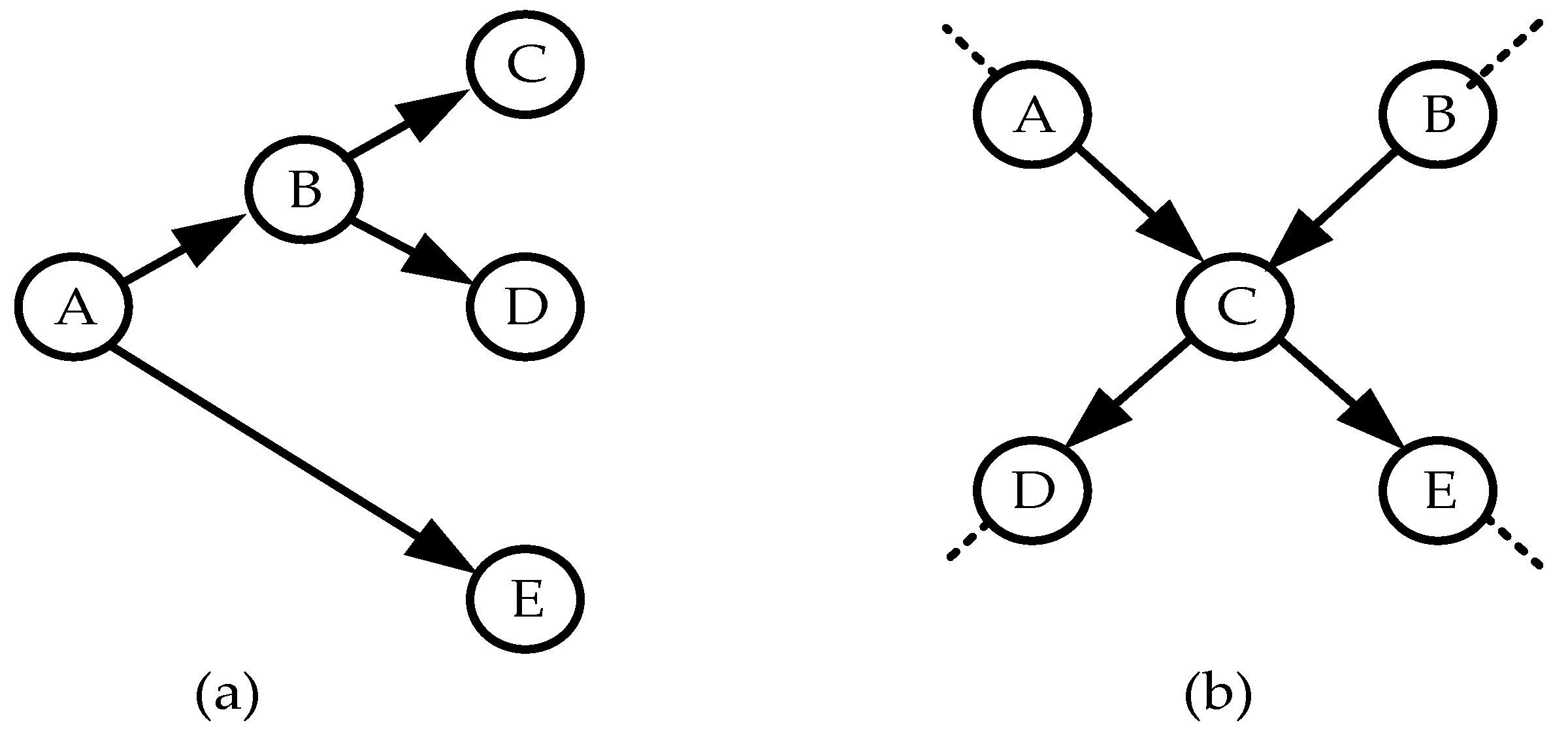
Let us present several provisions related to the syntax of Bayesian networks. The following characteristic types of connections between nodes in any Bayesian network can be defined (see Figure 1) (Korb and Nicholson 2011).
In Figure 1a, nodes A , B , C are connected in a series (chain connection). This type of relationship indicates that the probabilities of events in node B depend on events in node A , and the probabilities of events in node C depend on events in node B . It can be argued that the probabilities of events in node C depend on events in node A , but not directly, but only through events in node B .
Figure 1b shows the divergent type of connections. The probabilities of events at nodes B and C depend on events in node A . In this sense, we can say that nodes B and C have a common cause, node A . Naturally, the concept of a common cause can be extended to several nodes greater than two.
Figure 1c shows the convergent type of connections. The probabilities of events at node C depend on both events at node A and events at node B . Here we can say that variable C has two causes. Naturally, the number of causes may be more than two.
The following terminology is used for Bayesian network structures. If nodes A and B are connected by an arc emanating from node A , then node A is called the direct predecessor (parent) of node B , and node B is called the direct successor (child) of node A . Figure 1b shows a situation where node A has two children: nodes B and C . Figure 1c shows the situation when node C has two parents: nodes A and B .
Based on the shapes of their structure, the following types of Bayesian networks can be distinguished (see Figure 2).
Figure 2a shows an example of a tree-like Bayesian network. The characteristic features of the structures of such networks are: (1) each network’s node has only one parent; (2) there is only one path between the starting node (the root of the tree) and any terminal node (the leaf of the tree).
Figure 2b shows a fragment of a conditional simply connected Bayesian network. In this type of network, some intermediate or terminal node may have more than one parent (nodes A and B are the parents of node C ).
Let us present the main provisions of the semantics of Bayesian networks. The probabilities of events represented by the initial nodes of the network are unconditionally independent. Otherwise, the probabilities of these events do not depend on any events in other network nodes. But if an event occurs in a certain parent node, then the events in the nodes that are children of this node become conditionally independent. Thus, if in node C in Figure 2b some event occurred, then the events in nodes A and B become conditionally independent. If in node A in Figure 2b some event occurred, then the probabilities of events in node C no longer are dependent on events in node A , but remain dependent on events in node B .
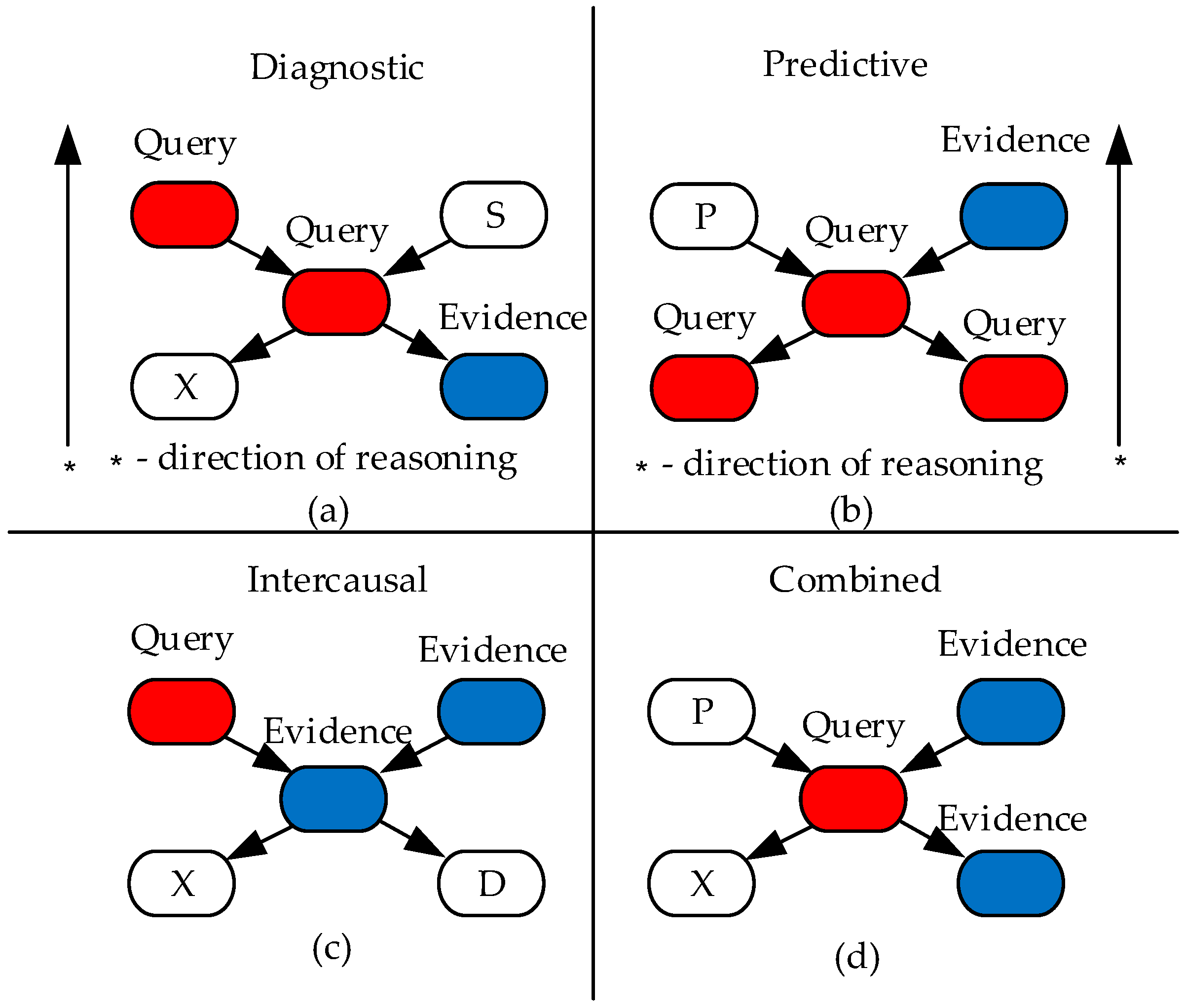
On a fully formed Bayesian network, the probabilistic inference problem of interest to us can be solved (alternatively, the type of reasoning can be implemented). Common types of probabilistic inference (reasoning) are schematically presented in Figure 3 (Korb and Nicholson 2011).
Figure 3a presents diagnostic inference. An example of such an inference would be re-estimating the probabilities of the causes of some disease if a patient is diagnosed with that disease. A characteristic feature of this type of inference is that the inference is made in the direction opposite to the direction of the arcs on the network.
Figure 3a presents diagnostic inference.
Figure 3b presents predictive inference. An example of such an inference would be a re-estimation of the probabilities of possible diseases in a patient when certain symptoms appear. A characteristic feature of this type of inference is that the inference is made in the direction of the network arcs.
Intercausal inference (Figure 3c) is used to re-estimate the probabilities of causes in the corresponding network nodes if some cause event occurred in one of the network nodes. An example of this type of inference would be a re-estimating the probabilities of possible causes of a patient’s illness if one of the causes is confidently established.
Combined inference (Figure 3d) is a combination of some of the above types of probabilistic inference.
How can probabilistic inference be analytically performed on some Bayesian network? Let some path from the initial to the terminal node of the network include n variables (nodes) Y 1 , Y 2 , , Y j , , Y n . Then the general probability distribution for this path can be represented as:
P ( Y 1 ,   .. , Y n ) = P ( Y 1 ) × P ( Y 2 / Y 1 ) × × P ( Y n / Y 1 , , Y n 1 ) = = j P ( Y j / Y 1 , , Y j 1 ) , j = 1 , , n .
Considering that the probabilities of events in an intermediate or terminal node of the network depend only on events in the parent node (nodes) of this node, expression (2) can be presented in the following generalized form:
P ( Y 1 , , Y n ) = j P ( Y j / P a r e n t s ( Y j ) ) ,
where P a r e n t s ( Y j ) is the set of parent nodes of node Y j .
It must be kept in mind that the probabilities of events at some intermediate or terminal node on a selected path may be dependent on events in other nodes that are the parents of this node but are not included in the selected path. Therefore, conditional probabilities of events in this node must be assigned over the entire set of its parents. If there are many such nodes with multiple parent nodes on the network, this greatly increases the number of required assignments and calculations.
It follows that direct calculations to determine the general probability distribution on the network using expression (2) are computationally expensive. To simplify and unify the required calculations, the probability propagation algorithm (Pearl 1988; Neapolitan 1990, 2004) is widely used. We will present a fuzzy version of this algorithm in the next section.
More information about probabilistic inference on Bayesian networks can be found in (Castillo et al. 1997; Jensen and Nielsen 2007; Jordan 1997; Lauritzen 2020; Stephenson 2000). Information on the practical application of Bayesian networks can be found in (Belza and Larrañaga 2014; Favaretto 2024).

4. Fuzzy Version of the Pearl’s Algorithm

In a classical version of Pearl’s algorithm, calculations of a priori and posteriori probabilities of events in network nodes are performed by spreading of λ -estimates and π -estimates vectors throughout the network. It is assumed that all initial and calculated probability values in networks nodes are deterministic values and λ -estimates and π -estimates are also uniquely determined.
In essence, the concepts λ -estimates, π -estimates, λ -values, and π -values are artificial entities. They are introduced for the purpose of formally using the Pearl algorithm. These estimates and values are established, calculated distributed according to the rules of the algorithm. The transition from λ -values and π -values to real estimates of probabilities in the relevant nodes of the network is also carried out according to the rules of the algorithm.
In this section we present a fuzzy version of the Pearl’s algorithm. The values of the relevant probabilities are represented in the form of triangular normal fuzzy numbers. The values of estimates distributed over the network are also represented in the form of triangular normal fuzzy numbers. Since, when performing calculation procedures, the values of some estimates and values are set equal to 1, we use a conditional fuzzy value 1 ˜ = ( 1 , 1 , 1 ) to unify definitions and calculation procedures.
When applying the proposed fuzzy version of this algorithm, the problem of normalizing the resulting fuzzy probability values arises. To normalize the crisp resulting probability values, each of the probability values from the set of calculated probabilities in some network node is simply divided by the sum of these probabilities. Thus, the initial probability values are normalized.
The conditions for normalizing fuzzy probability values are formulated in a more complex way. Let there be a complete group of n random events. The values of these probabilities are given in the form of triangular normal fuzzy numbers p ˜ i = ( l i , m i , u i ) , i = 1 , , n , where l i is the lower bound of the fuzzy number p ˜ i basis, m i is the probability value for which μ ( p ˜ i ) = 1 , and u i is the upper bound of the fuzzy number p ˜ i basis.
Let us formulate the conditions under which the values p ˜ i are normalized fuzzy values.
  • The sum of the central values of m fuzzy numbers must be equal to 1:
    i = 1 n m i = 1 .
  • Fuzzy number bases p ˜ i should be reachable intervals (De Campos et al. 1994):
    i , j i l j + u i 1 ;
    i , j i u j + l i 1 .
If condition (4) is not satisfied for the set of fuzzy probabilities { p ˜ i / i = 1 , , n } under consideration, then new values m i are calculated using the expression
m i = m i i = 1 n m i
Let us denote the bases boundaries of fuzzy probability values p ˜ i by [ l i , u i ] , i = 1 , , n . These intervals are equal in size to the original intervals [ l i , u i ] , but are shifted along the axis p according to the changed values m i .
If conditions (5), (6) are not met for the transformed set of fuzzy probability values { p ˜ i / i = 1 , , n } , then the new values of the bases’ boundaries of the relevant fuzzy probability values are recalculated using the expressions (De Campos et al. 1994)
i , l i = max [ l i , 1 i j u j ]
i , u i = min [ u i , 1 j i l j ]
In a general sense, normalization of fuzzy probabilities means that it is always possible to choose such crisp values of probabilities on the bases of the corresponding fuzzy numbers that will be normalized, that is, their sum is equal to 1. From expressions (8) and (9) it immediately follows that this condition is satisfied for the boundary values of the bases of the relevant fuzzy numbers. From expression (7), it directly follows that this condition is satisfied for the central values of the relevant fuzzy values. It follows from this that, on the bases of the corresponding fuzzy numbers, a set of normalized clear probability values can always be formed. To simplify the problem of selecting the crisp probability values that interest us, the algorithm proposed in (Uzhga-Rebrov 2019) can be used. Using this algorithm, a set of normalized crisp probability values of interest to us can be selected for cases of three and four fuzzy probability values.
To avoid potential normalization of the original fuzzy probability values, it may be recommended to assign these estimates in the form of consistent fuzzy values (Uzhga-Rebrov 2016): (1) i = 1 n m i = 1 ; (2) all the bases of the corresponding fuzzy numbers are the same.
There is another method for normalizing fuzzy probability values:
p ˜ j = p ˜ j = 1 n p ˜ j .
However, this method gives wider intervals for the bases of fuzzy normalized probability values. Therefore, normalization by expressions (7)–(9) seems to be preferable, and it will be used in this work.
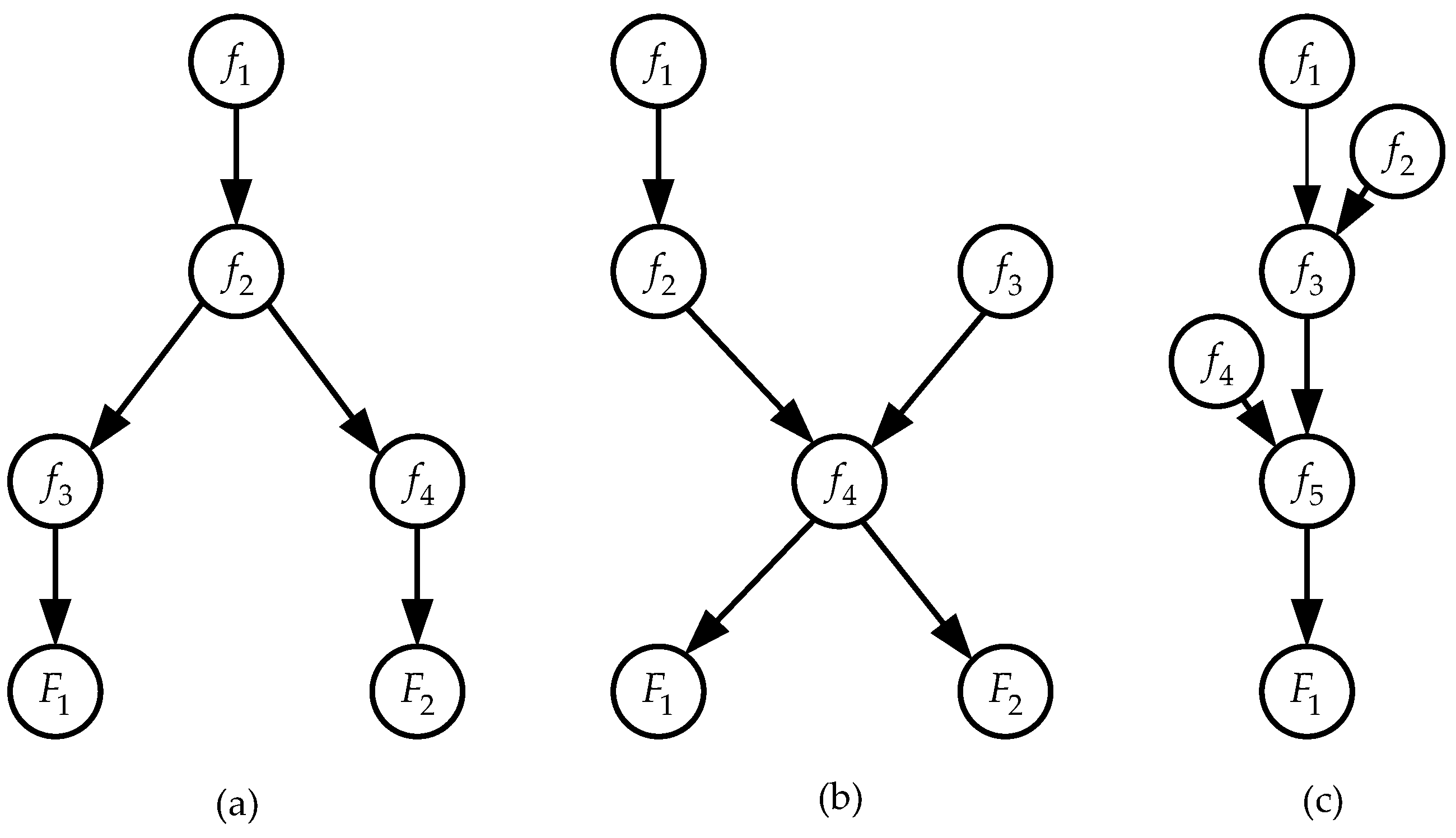
Let us present characteristic types of simply connected Bayesian networks that can represent connections between subfactors and factors in problems of probabilistic risk assignment (Figure 4).
Figure 4a shows a tree-like Bayesian network. Subfactor f 1 states influence the probabilities of subfactor f 2 states. Subfactor f 2 states influence the probabilities of subfactor f 3 , f 4 states. In turn, the states of the subfactor f 3 influence the probabilities of the states of the factor F 1 , and the states of the subfactor f 4 influence the probabilities of the states of the factor F 2 . This type of connection between subfactors and factors is quite rare in problems of probabilistic assignment of environmental risks.
Figure 4b shows the convergent-divergent type of connections between subfactors and factors. The probabilities of the subfactor f 2 states depend on the subfactor f 1 states. The probabilities of subfactor f 4 states depend on the states of subfactors f 2 , f 3 . The probabilities of the states of the factors F 1 and F 2 depend on the states of the subfactor f 4 .
In Figure 4c, the subfactors f 1 , f 3 , f 5 and factor F nodes are connected in a chain manner. Additionally, the probabilities of subfactor f 3 states are influenced by subfactor f 2 states, and the probabilities of subfactor f 5 states are influenced by subfactor f 4 states. The structure of this network may be called a “reverse tree”, but this network is a typical example of a simply connected network. Note that this type of network structure is the most common in problems of probabilistic assignment of environmental risks.
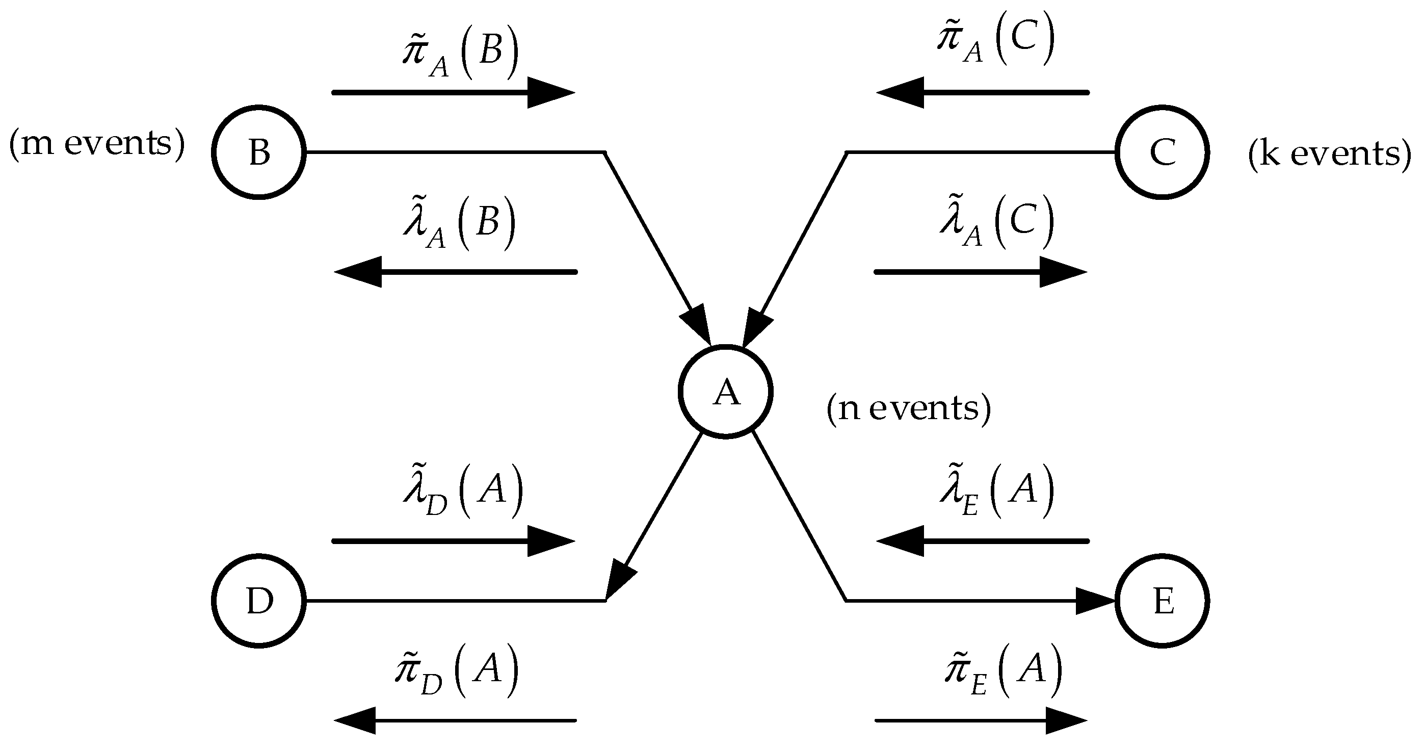
We will present a fuzzy version of Pearl’s probability propagation algorithm on a Bayesian network, taking as a basis the network fragment in Figure 5.
The choice of this structure is because this structure simultaneously reflects both the convergent and divergent type of connections between nodes. The inference algorithm presented below for this network fragment is applicable to any other types of Bayesian networks. To calculate all fuzzy values of total probabilities in some intermediate network node (node A in Figure 5), this node must receive a vector of fuzzy λ ˜ -estimates λ ˜ D ( A ) , λ ˜ E ( A ) from its direct successors (children)—nodes D and E —and vectors of fuzzy π ˜ -estimates, π ˜ A ( B ) , π ˜ A ( C ) , from their direct predecessors (parents)—nodes B and C . After performing the necessary calculations in node A , vectors of fuzzy π ˜ -estimates π ˜ D ( A ) , π ˜ E ( A ) can be sent to nodes D and E and a vector of fuzzy λ ˜ -estimates λ ˜ D ( A ) , λ ˜ E ( A ) to nodes B and C . The necessary calculation expressions will be presented in subsequent definitions. We combine algorithms for propagating fuzzy prior and posterior probabilities over the network. To do this, let Z denote the set of nodes in which events occurred.
Definition 1 (fuzzy  λ ˜  estimates).
Let node  A , displaying  n  events, have two direct predecessors (parents): node  B , displaying  m  events, and node  C , displaying  k  events (see Figure 5). Then for  1 i m
λ ˜ A ( b i ) = l = 1 k ( π ˜ A ( c l ) ) j = 1 n p ˜ ( a j / b i , c l ) λ ˜ ( a j ) , i = 1 , , m ,
where  p ˜ ( a j / b i , c l )  is the fuzzy conditional probability of an event  a j  occurring, subject to the simultaneous occurrence of events  b i  and  c l  ;  π ˜ A ( c l )  is given in Definition 3;  λ ˜ ( a j )  is given in Definition 2.
If node  A  has only one parent, node  B , then the value  λ ˜ ( b i )  is calculated by the expression:
λ ˜ A ( b i ) = j = 1 n p ˜ ( a j / b i ) λ ˜ ( a j ) , i = 1 , , m .
The complete vector of estimates λ ˜ A ( b i ) for everyone 1 i m is called a fuzzy λ ˜ -estimate from A to B and is denoted by λ ˜ A ( B ) .
Definition 2 (fuzzy  λ ˜ -values).
Let  Z  be a subset of nodes in which events occurred,  A  be a node displaying  n  events, and  B k  ,  k = 1 , 2 ,  be the direct successors (children) of node  A . Then:
If  A Z  and  A  is also a terminal node, then
λ ˜ ( a j ) = 1 ˜ , j = 1 , , n .
If  A Z  and  A  is also an intermediate or initial node, then
λ ˜ ( a j ) = B k λ ˜ B k ( a j ) , j = 1 , , n .
If  A Z  and  A  is an arbitrary network node, then
λ ˜ ( a j ) = 1 ˜ , if   event   a j   is   occurred .
λ ˜ ( a ) = 0 , if   event   a i 1 , , n , i j ,   is   occurred .
The complete vector of values λ ˜ ( a j ) , 1 j n , is called the fuzzy λ ˜ -value A and is denoted by λ ˜ ( A ) .
Definition 3 (fuzzy  π ˜ -estimates).
Let  Z  be a subset of nodes in which events occurred,  A  be an arbitrary initial or intermediate network node reflecting  n  events, and  B  be a direct successor (child) of node  A . Then:
If  A Z  , then
π ˜ B ( a j ) = p ˜ ( a / Z ) / λ ˜ B ( a j ) ,
where  p ˜ ( a j / Z )  is the current fuzzy value of the probability of the event  a j  occurring;  λ ˜ B ( a j )  —is given in Definition 1.
If  A Z  , then
π ˜ B ( a j ) = 1 ˜ , if   event   a j   is   occurred ;
π ˜ B ( a j ) = 0 , if   event   a i 1 , , n , i j ,   is   occurred .
If node  A  has a set of nodes  B k  as direct successors (children),  k = 1 , 2 ,  , then  π ˜ -estimates are calculated for each node either by expression (15) or by expression (16).
The complete vector of fuzzy estimates π ˜ B ( a j ) for 1 j n is called a fuzzy π ˜ -estimate from A to B and is denoted by π ˜ B ( A ) .
Definition 4 (fuzzy  π ˜ -values).
Let  A  be an arbitrary network node containing  n  events. Then:
If node  A  is an arbitrary intermediate or terminal node of the network, and it has direct predecessors (parents) node  B  , displaying  m  events, and node  C  , having  k  events (see Figure 5), then for   1 i n
π ˜ ( a i ) = j = 1 m l = 1 k ( p ˜ ( a i / b j , c l ) ) π ˜ A ( b j ) π ˜ A ( c l )
where  p ˜ ( a i / b j , c l )  is the fuzzy conditional probability of an event  a i  occurring, subject to the simultaneous occurrence of events  b j  and  c l ;  π ˜ A ( b j )  ,  π ˜ A ( c l )  are given in Definition 3.
If node  A  has only one direct predecessor (parent), node  B  , then expression (12a) takes the form
π ˜ ( a i ) = j = 1 m p ˜ ( a i / b j ) π ˜ A ( b j ) .
If node  A  is the initial node of the network, then for  1 i n
π ˜ ( a i ) = p ˜ ( a i ) ,
where  p ˜ ( a i )  is the fuzzy value of the unconditional probability of the event  a i  occurring.
The complete vector of values π ˜ ( a i ) is called the fuzzy π ˜ -value A and is denoted by π ˜ ( A ) .
Definition 5 (fuzzy complete conditional probabilities). 
Let  Z  be a subset of nodes where events occurred and  A  be an arbitrary network node containing  n  events. Then for  1 i n
p ˜ ( a i / Z ) = ( φ A ) λ ˜ ( a i ) π ˜ ( a i ) ,
where the symbol  ( φ A )  denotes the procedures for normalizing the calculated fuzzy values  p ˜ ( a i / Z )  using expressions (7)–(9).
Note that normalization procedures are performed only in those cases when the calculated fuzzy values p ˜ ( a i / Z ) are not normalized.
Let us present the steps and procedures of the fuzzy probability propagation algorithm on simply connected Bayesian networks. Let all initial unconditional and conditional fuzzy probability values be specified in all network nodes. First, without considering whether certain events occurred or did not occur in individual nodes of the network, a priori fuzzy conditional probabilities are propagated throughout the network. To do this, the following steps of the algorithm are performed.
Step S.1. For λ ˜ -values, λ ˜ -estimates, and π ˜ -estimates, set the values equal to 1 ˜ .
Step S.2. For events in all the initial nodes of the network, π ˜ -values are set equal to the fuzzy values of the a priori unconditional probabilities of these events: π ˜ ( a j i ) = p ˜ ( a j i ) , where j is the node number and i is the event number in the j -th node.
If no event occurs in any network node, then the following steps of the algorithm are performed:
Step S.3. New π ˜ -estimates are sent to all direct successors (children) of the initial nodes according to expression (15).
Step S.4. Fuzzy π ˜ -values are calculated for events in nodes that are direct successors (children) of the initial nodes using expressions (17) or (18).
Step S.5. Fuzzy a priori conditional probabilities of events in nodes that are direct successors (children) of the initial nodes are calculated using expression (20).
Steps S.3, S.4, and S.5 are sequentially repeated for all nodes in the direction of the network arcs until all terminal nodes are reached.
If an event occurred at some node A , or node A received new λ ˜ -estimates, or new π ˜ -estimates provided that Z , then one of the following procedures is performed:
Procedure A. If an event a j occurs in node A , then:
Step A.1. Set p ˜ ( a j ) = 1 ˜ and p ˜ ( a i ) = 0 , i 1 , , n ,   i j .
Step A.2. Set the value λ ˜ ( A ) according to the expression (13).
Step A.3. Send new λ ˜ -estimates to all direct predecessors (parents) of node A according to expression (11) in the case of one parent node and according to expression (10) for the case of multiple parents of node A .
Step A.4. Send new π ˜ -estimates to all direct successors (children) of node A using expression (16).
Procedure B. If A Z (no event occurred at node A ) and node A received new λ ˜ -estimates from all its direct successors (children), then:
Step B.1. Calculate new values λ ˜ ( A ) using the expression (13).
Step B.2. If new values π ˜ ( A ) are known, calculate the value of the vector ( p ˜ ( A ) ) using expression (20).
Step B.3. Send new λ ˜ -estimates to all direct predecessors (parents) of node A using expressions (10) or (11), respectively.
Step B.4. Send new π ˜ -estimates to all direct successors (children) of node A using expression (16).
Procedure C. A Z (no event occurred at node A ) and node A received new π ˜ -estimates from all its direct predecessors (parents), then:
Step C.1. Calculate new values π ˜ ( A ) using expressions (17) or (18), respectively.
Step C.2. If the value λ ˜ ( A ) is known, calculate the values of the vector ( p ˜ ( A ) ) using expression (20).
Step C.3. Send new π ˜ -estimates to all direct successors (children) of node A using expression (15).
Step C.4. If λ ˜ ( A ) ( 1 ˜ , , 1 ˜ ) , send new λ ˜ -estimates to all direct predecessors (parents) of node A using expressions (10) or (11).

5. Illustrative Example

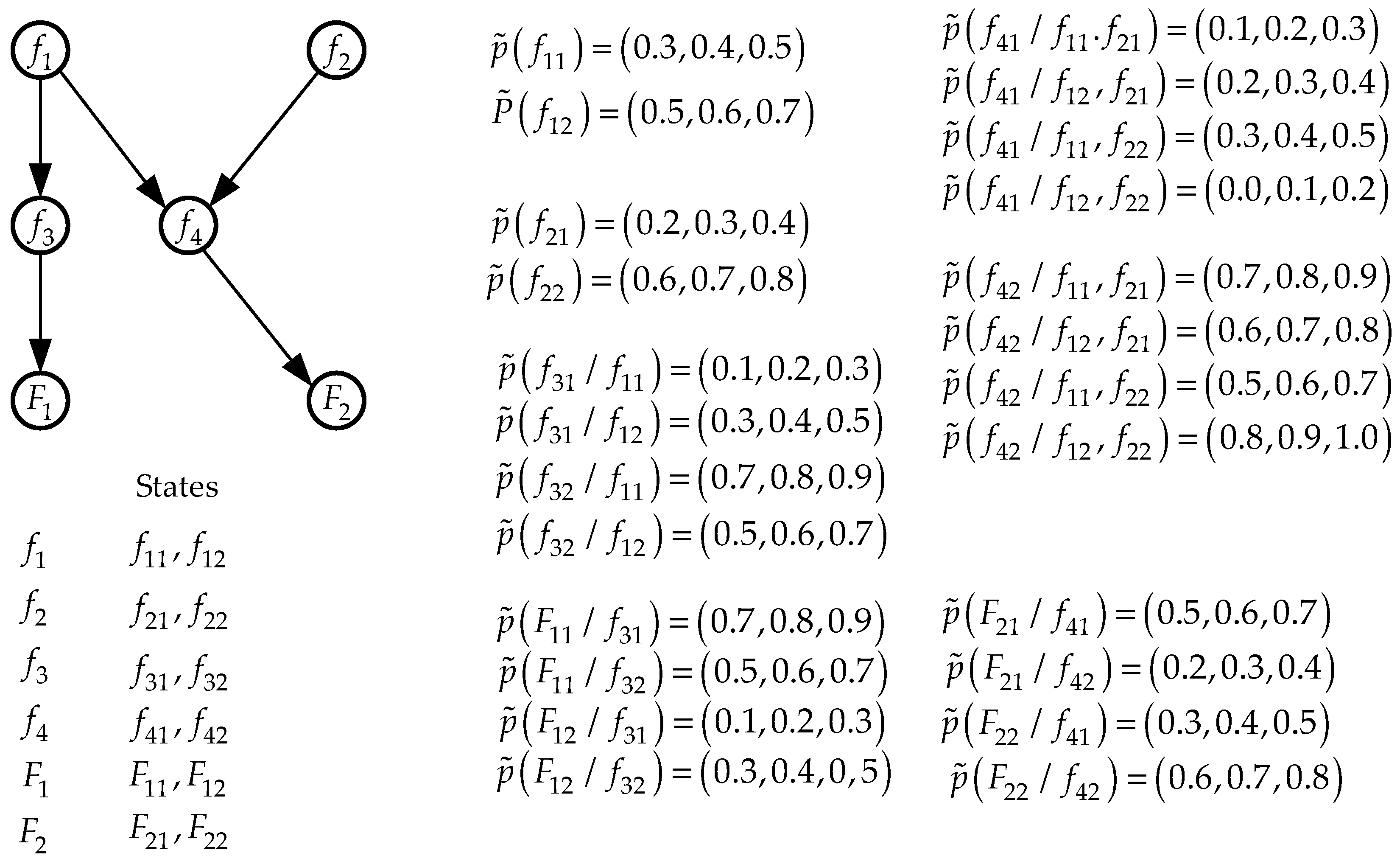
We will demonstrate the use of a fuzzy version of the Pearl’s probability propagation algorithm on the simple Bayesian network shown in Figure 6. In this figure, the nodes F 1 , F 2 display the states of relevant factors and the nodes f 1 ,   f 2 ,   f 3 ,   f 4 display the states of the subfactors associated with them. All assigned probability values for the states of factors and subfactors are consistent fuzzy values. Therefore, by definition, they are normalized fuzzy values.
Note that the requirement of consistency of initial fuzzy probability values is not a mandatory requirement. The consistency condition means that the fuzzy probabilities of the states of factors and subfactors are assigned with the same degrees of uncertainty. If the initial fuzzy probability values are not consistent, a check for normalization conditions (4), (5) is required and, if necessary, these values must be normalized using expressions (6), (8) (9).
Let us carry out the initial steps of assignments, provided that no event has occurred in any network node (the state of the corresponding factor has not changed) ( Z = ) .
S.1.
λ ˜ ( f 1 ) = ( 1 ˜ , 1 ˜ ) , λ ˜ ( f 2 ) = ( 1 ˜ , 1 ˜ ) , λ ˜ ( f 3 ) = ( 1 ˜ , 1 ˜ ) , λ ˜ ( f 4 ) = ( 1 ˜ , 1 ˜ ) , λ ˜ ( F 1 ) = ( 1 ˜ , 1 ˜ ) , λ ˜ ( F 2 ) = ( 1 ˜ , 1 ˜ ) , λ ˜ F 1 ( f 3 ) = ( 1 ˜ , 1 ˜ ) , λ ˜ F 2 ( f 4 ) = ( 1 ˜ , 1 ˜ ) , λ ˜ f 3 ( f 1 ) = ( 1 ˜ , 1 ˜ ) , λ ˜ f 4 ( f 1 ) = ( 1 ˜ , 1 ˜ ) , λ ˜ f 4 ( f 2 ) = ( 1 ˜ , 1 ˜ ) , π ˜ f 3 ( f 1 ) = ( 1 ˜ , 1 ˜ ) , π ˜ f 4 ( f 1 ) = ( 1 ˜ , 1 ˜ ) , π ˜ f 2 ( f 3 ) = ( 1 ˜ , 1 ˜ ) , π ˜ F 1 ( f 2 ) = ( 1 ˜ , 1 ˜ ) , π ˜ F 2 ( f 4 ) = ( 1 ˜ , 1 ˜ ) .
S.2.
π ˜ ( f 1 ) = ( ( 0.3 , 0.4 , 0.5 ) , ( 0.5 , 0.6 , 0.7 ) ) ; π ˜ ( f 2 ) = ( ( 0.2 , 0.3 , 0.4 ) , ( 0.6 , 0.7 , 0.8 ) ) .
S.3.
π ˜ f 3 ( f 11 ) = p ˜ ( f 11 ) / λ ˜ ( f 11 ) = ( 0.3 ,   0.4 ,   0.5 ) / 1 ˜ = ( 0.3 ,   0.4 ,   0.5 ) ; π ˜ f 3 ( f 12 ) = p ( f 12 ) / λ ˜ ( f 12 ) = ( 0.5 ,   0.6 ,   0.7 ) / 1 ˜ = ( 0.5 ,   0.6 ,   0.7 ) . π ˜ f 4 ( f 11 ) = p ˜ ( f 11 ) / λ ˜ f 4 ( f 11 ) = ( 0.3 ,   0.4 ,   0.5 ) / 1 ˜ = ( 0.3 ,   0.4 ,   0.5 ) ; π ˜ f 4 ( f 12 ) = p ( f 12 ) / λ ˜ f 4 ( f 12 ) = ( 0.5 ,   0.6 ,   0.7 ) / 1 ˜ = ( 0.5 ,   0.6 ,   0.7 ) . π ˜ f 4 ( f 21 ) = p ˜ ( f 21 ) / λ ˜ f 4 ( f 21 ) = ( 0.2 ,   0.3 ,   0.4 ) / 1 ˜ = ( 0.2 ,   0.3 ,   0.4 ) ; π ˜ f 4 ( f 22 ) = p ( f 22 ) / λ ˜ f 4 ( f 22 ) = ( 0.6 ,   0.7 ,   0.8 ) / 1 ˜ = ( 0.6 ,   0.7 ,   0.8 ) .
For the node f 3 steps S.4, S.5, S.3 can now be performed:
S.4.
π ˜ ( f 31 ) = p ˜ ( f 31 / f 11 ) π ˜ f 3 ( f 11 ) + p ˜ ( f 31 / f 12 ) π ˜ f 3 ( f 12 ) = = ( 0.1 ,   0.2 ,   0.3 ) ( 0.3 ,   0.4 ,   0.5 ) + ( 0.3 ,   0.4 ,   0.5 ) ( 0.5 ,   0.6 ,   0.7 ) = = ( 0.03 ,   0.08 ,   0.15 ) + ( 0.15 ,   0.24 ,   0.35 ) = ( 0.18 ,   0.32 ,   0.50 ) . π ˜ ( f 32 ) = p ˜ ( f 32 / f 11 ) π ˜ f 3 ( f 11 ) + p ˜ ( f 32 / f 12 ) π ˜ f 3 ( f 12 ) = = ( 0.7 ,   0.8 ,   0.9 ) ( 0.3 ,   0.4 ,   0.5 ) + ( 0.5 ,   0.6 ,   0.7 ) ( 0.5 ,   0.6 ,   0.7 ) = = ( 0.21 ,   0.32 ,   0.45 ) + ( 0.25 ,   0.36 ,   0.49 ) = ( 0.46 ,   0.68 ,   0.94 ) .
S.5.
p ˜ ( f 31 ) = λ ˜ ( f 31 ) π ˜ ( f 31 ) = 1 ˜ ( 0.18 ,   0.32 ,   0.50 ) = ( 0.18 ,   0.32 ,   0.50 ) ; p ˜ ( f 32 ) = λ ˜ ( f 32 ) π ˜ ( f 32 ) = 1 ˜ ( 0.46 ,   0.68 ,   0.94 ) = ( 0.46 ,   0.68 ,   0.94 ) .
For the calculated fuzzy probability values, the normalization condition (4) is satisfied. Let us check the fulfilment of the normalization condition (5).
0.18 + 0.94 = 1.12 > 1 ;   0.46 + 0.50 = 0.96 < 1 .
The normalization condition (5) is not satisfied. Let us check whether the normalization condition (6) is satisfied.
0.50 + 0.46 = 0.96 < 1 ;   0.94 + 0.18 = 1.12 > 1 .
The normalization condition (6) is not satisfied. Let us transform the boundaries of the bases of fuzzy numbers p ˜ ( f 31 ) , p ˜ ( f 32 ) according to the expressions (8), (9).
p ˜ ( f 31 ) l 1 = max [ 0.18 , 1 0.94 ] = max [ 0.18 , 0.06 ] = 0.18 ; u 2 = min [ 0.50 , 1 0.46 ] = min [ 0.50 , 0.54 ] = 0.50 .
p ˜ ( f 32 ) l 2 = max [ 0.46 , 1 0.50 ] = max [ 0.46 , 0.50 ] = 0.50 ; u 2 = min [ 0.94 , 1 0.18 ] = min [ 0.94 , 0.82 ] = 0.82 .
Finally, we have:
p ˜ ( f 21 ) = ( 0.18 ,   0.32 ,   0.50 ) ;   p ˜ ( f 32 ) = ( 0.50 ,   0.68 ,   0.82 ) .
S.3.
π ˜ F 1 ( f 31 ) = p ˜ ( f 31 ) / λ ˜ F 1 ( f 31 ) = ( 0.18 ,   0.32 ,   0.50 ) / 1 ˜ = ( 0.18 ,   0.32 ,   0.50 ) ; π ˜ F 1 ( f 32 ) = p ( f 32 ) / λ ˜ F 1 ( f 32 ) = ( 0.50 ,   0.68 ,   0.82 ) / 1 ˜ = ( 0.50 ,   0.68 ,   0.82 ) .
Node F1.
S.4.
π ˜ ( F 11 ) = p ˜ ( F 11 / f 31 ) π ˜ F 1 ( f 31 ) + p ˜ ( F 11 / f 32 ) π ˜ F 1 ( f 32 ) = = ( 0.70 ,   0.80 ,   0.90 ) ( 0.18 ,   0.32 ,   0.50 ) + ( 0.50 ,   0.60 ,   0.70 ) ( 0.50 ,   0.68 ,   0.82 ) = = ( 0.126 ,   0.256 ,   0.450 ) + ( 0.300 ,   0.408 ,   0.574 ) = ( 0.426 ,   0.664 ,   1.024 ) ; π ˜ ( F 12 ) = p ˜ ( F 12 / f 31 ) π ˜ F 1 ( f 31 ) + p ˜ ( F 12 / f 32 ) π ˜ F 1 ( f 32 ) = = ( 0.10 ,   0.20 ,   0.30 ) ( 0.18 ,   0.32 ,   0.50 ) + ( 0.30 ,   0.40 ,   0.50 ) ( 0.50 ,   0.68 ,   0.82 ) = = ( 0.018 ,   0.064 ,   0.150 ) + ( 0.150 ,   0.272 ,   0.410 ) = ( 0.168 ,   0.336 ,   0.560 ) .
S.5.
p ˜ ( F 11 ) = λ ˜ ( F 11 ) π ˜ ( F 11 ) = 1 ˜ ( 0.426 ,   0.664 ,   1.024 ) = ( 0.426 ,   0.664 ,   1.024 ) ; p ˜ ( F 12 ) = λ ˜ ( F 12 ) π ˜ ( F 12 ) = 1 ˜ ( 0.168 ,   0.336 ,   0.560 ) = ( 0.168 ,   0.336 ,   0.560 ) .
The normalization condition (4) for fuzzy estimates p ˜ ( F 11 ) , p ˜ ( F 12 ) is satisfied, but the normalization conditions (5), (6) are not satisfied. Using expressions (8), (9), we transform the boundaries of the bases of these fuzzy estimates.
p ˜ ( F 11 ) l 1 = max [ 0.426 , 1 0.560 ] = max [ 0.426 , 0.440 ] = 0.440 ; u 1 = min [ 1.024 , 1 0.168 ] = min [ 1.024 , 0.832 ] = 0.832 .
p ˜ ( F 12 ) l 2 = max [ 0.168 , 1 1.024 ] = max [ 0.168 , ( 0.024 ) ] = 0.168 ; u 2 = min [ 0.560 , 1 0.420 ] = min [ 0.560 , 0.580 ] = 0.560 .
Finally, we have:
p ˜ ( F 11 ) = ( 0.440 ,   0.664 ,   0.832 ) ;   p ˜ ( F 2 ) = ( 0.168 ,   0.336 ,   0.560 ) .
Node f 4 .
This node is a direct successor (child) of nodes f 1 and f 2 . Let us perform the necessary steps of the algorithm for this node.
S.4.
π ˜ ( f 41 ) = p ˜ ( f 41 / f 11 , f 21 ) π ˜ f 4 ( f 11 ) π ˜ f 4 ( f 21 ) + p ˜ ( f 41 / f 11 , f 22 ) π ˜ f 4 ( f 11 ) π ˜ f 4 ( f 22 ) + + p ˜ ( f 41 / f 12 , f 21 ) π ˜ f 4 ( f 12 ) π ˜ f 4 ( f 21 ) + p ˜ ( f 41 / f 12 , f 22 ) π ˜ f 4 ( f 12 ) π ˜ ( f 22 ) = = ( 0.1 ,   0.2 ,   0.3 ) ( 0.3 ,   0.4 ,   0.5 ) ( 0.2 ,   0.3 ,   0.4 ) + + ( 0.3 ,   0.4 ,   0.5 ) ( 0.3 ,   0.4 ,   0.5 ) ( 0.6 ,   0.7 ,   0.8 ) + + ( 0.2 ,   0.3 ,   0.4 ) ( 0.5 ,   0.6 ,   0.7 ) ( 0.2 ,   0.3 ,   0.4 ) + + ( 0.0 ,   0.1 ,   0.2 ) ( 0.5 ,   0.6 ,   0.7 ) ( 0.6 ,   0.7 ,   0.8 ) = = ( 0.006 ,   0.024 ,   0.060 ) + ( 0.054 ,   0.112 ,   0.200 ) + ( 0.020 ,   0.054 ,   0.112 ) + + ( 0.000 ,   0.042 ,   0.112 ) = ( 0.080 ,   0.233 ,   0.484 ) ; π ˜ ( f 42 ) = p ˜ ( f 42 / f 11 , f 21 ) π ˜ f 4 ( f 11 ) π ˜ f 4 ( f 21 ) + p ˜ ( f 42 / f 11 , f 22 ) π ˜ f 4 ( f 11 ) π ˜ f 4 ( f 22 ) + + p ˜ ( f 42 / f 12 , f 21 ) π ˜ f 4 ( f 12 ) π ˜ f 4 ( f 21 ) + p ˜ ( f 42 / f 12 , f 22 ) π ˜ f 4 ( f 12 ) π ˜ ( f 22 ) = = ( 0.7 ,   0.8 ,   0.9 ) ( 0.3 ,   0.4 ,   0.5 ) ( 0.2 ,   0.3 ,   0.4 ) + + ( 0.5 ,   0.6 ,   0.7 ) ( 0.3 ,   0.4 ,   0.5 ) ( 0.6 ,   0.7 ,   0.8 ) + + ( 0.6 ,   0.7 ,   0.8 ) ( 0.5 ,   0.6 ,   0.7 ) ( 0.2 ,   0.3 ,   0.4 ) + + ( 0.8 ,   0.9 ,   1.0 ) ( 0.5 ,   0.6 ,   0.7 ) ( 0.6 ,   0.7 ,   0.8 ) = = ( 0.042 ,   0.096 ,   0.180 ) + ( 0.090 ,   0.168 ,   0.280 ) + ( 0.060 ,   0.126 ,   0.224 ) + + ( 0.240 ,   0.378 ,   0.560 ) = ( 0.432 ,   0.768 ,   1.244 ) .
S.5.
p ˜ ( f 41 ) = λ ˜ ( f 41 ) π ˜ ( f 41 ) = 1 ˜ ( 0.080 ,   0.232 ,   0.484 ) ; p ˜ ( f 42 ) = λ ˜ ( f 42 ) π ˜ ( f 42 ) = 1 ˜ ( 0.432 ,   0.768 ,   1.244 ) .
Performing normalization of the obtained values according to the expression (8), (9), we finally have:
p ˜ ( f 41 ) = ( 0.080 ,   0.232 ,   0.484 ) ;   p ˜ ( f 42 ) = ( 0.516 ,   0.768 ,   0.920 ) .
S.3.
π ˜ F 2 ( f 41 ) = p ˜ ( f 41 ) / λ ˜ F 2 ( f 41 ) = ( 0.080 ,   0.232 ,   0.484 ) / 1 ˜ = ( 0.080 ,   0.232 ,   0.484 ) ; π ˜ F 2 ( f 42 ) = p ˜ ( f 42 ) / λ ˜ F 2 ( f 42 ) = ( 0.516 ,   0.768 ,   0.920 ) / 1 ˜ = ( 0.516 ,   0.768 ,   0.920 ) .
Node F 2 .
S.4.
π ˜ ( F 21 ) = p ˜ ( F 21 / f 41 ) π ˜ F 2 ( f 41 ) + p ˜ ( F 21 / f 42 ) π ˜ F 2 ( f 42 ) = = ( 0.5 ,   0.6 ,   0.7 ) ( 0.080 ,   0.232 ,   0.484 ) + ( 0.2 ,   0.3 ,   0.4 ) ( 0.516 ,   0.768 ,   0.920 ) = = ( 0.040 ,   0.139 ,   0.389 ) + ( 0.103 ,   0.230 ,   0.358 ) = ( 0.143 ,   0.369 ,   0.457 ) ; π ˜ ( F 22 ) = p ˜ ( F 22 / f 41 ) π ˜ F 2 ( f 41 ) + p ˜ ( F 22 / f 42 ) π ˜ F 2 ( f 42 ) = = ( 0.3 ,   0.4 ,   0.5 ) ( 0.080 ,   0.232 ,   0.484 ) + ( 0.6 ,   0.7 ,   0.8 ) ( 0.516 ,   0.768 ,   0.920 ) = = ( 0.024 ,   0.093 ,   0.242 ) + ( 0.310 ,   0.538 ,   0.736 ) = ( 0.334 ,   0.631 ,   0.978 ) .
S.5.
p ˜ ( F 21 ) = λ ˜ ( F 21 ) π ˜ ( F 21 ) = 1 ˜ ( 0.143 ,   0.369 ,   0.457 ) = ( 0.143 ,   0.369 ,   0.457 ) ; p ˜ ( F 22 ) = λ ˜ ( F 22 ) π ˜ ( F 22 ) = 1 ˜ ( 0.334 ,   0.631 ,   0.978 ) = ( 0.334 ,   0.631 ,   0.978 ) .
Performing normalization of the obtained fuzzy estimates by expressions (8), (9), we finally have:
p ˜ ( F 21 ) = ( 0.143 ,   0.369 ,   0.437 ) ;   p ˜ ( F 22 ) = ( 0.543 ,   0.631 ,   0.857 ) .
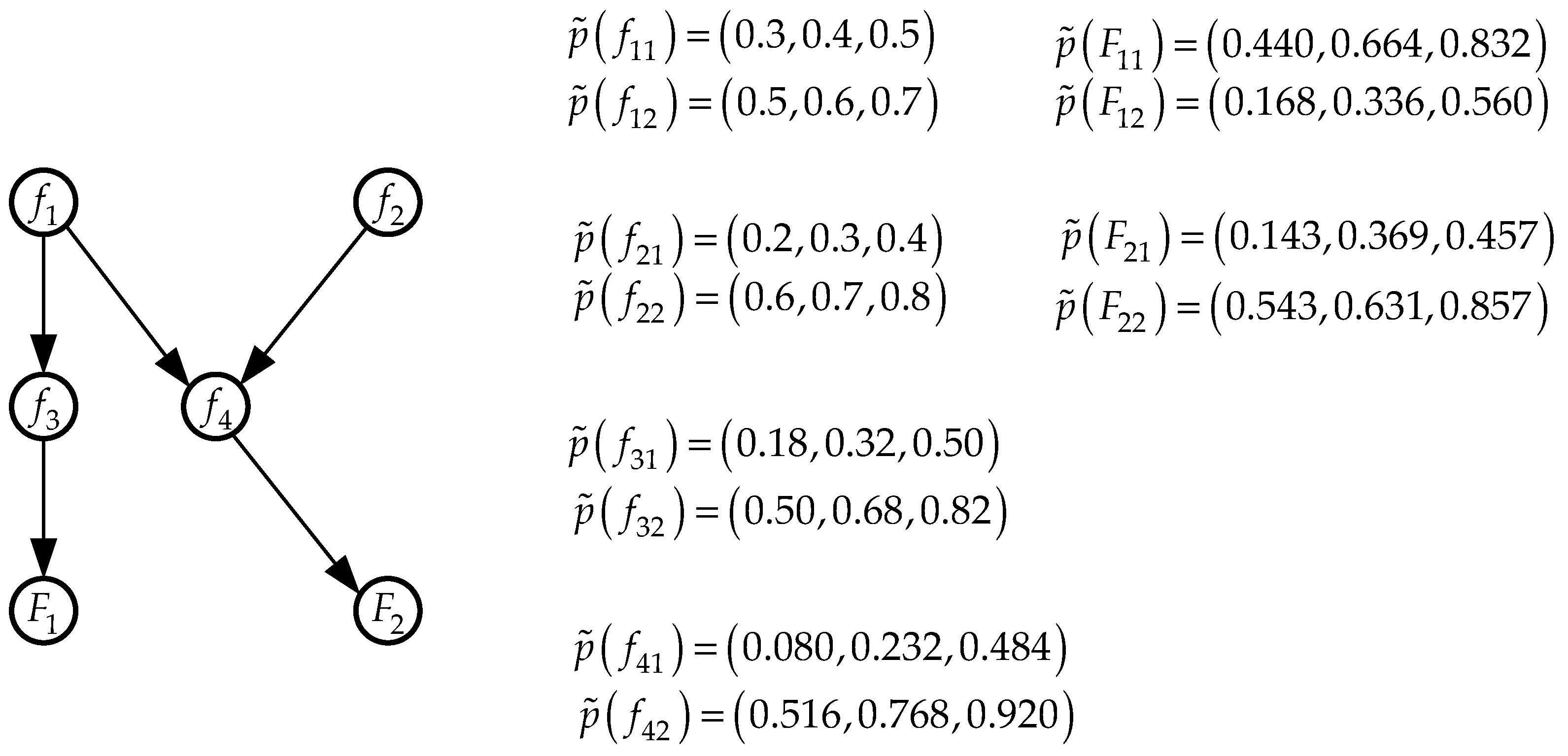
The propagation of prior probabilities is complete. Re-estimated probabilities of subfactor and factor states from the Bayesian network in Figure 6 are shown in Figure 7.
Let us assume that an event occurred in the node f 4 (the state f 41 of the factor f 4 was realized). Now the sequence of A algorithm procedures can be applied to this node.
Node f 4 .
A.1.
p ˜ ( f 41 ) = 1 ˜ ; p ˜ ( f 42 ) = 0 .
A.2.
λ ˜ ( f 41 ) = 1 ˜ ; λ ˜ ( f 42 ) = 0 .
A.3.
λ ˜ f 4 ( f 11 ) = π ˜ f 4 ( f 21 ) [ p ˜ ( f 41 / f 11 , f 21 ) λ ˜ ( f 41 ) + p ˜ ( f 42 / f 11 ,   f 21 ) λ ˜ ( f 42 ) ] + + π ˜ f 4 ( f 22 ) [ p ˜ ( f 41 / f 11 , f 22 ) λ ˜ ( f 41 ) + p ( f 42 / f 11 , f 22 ) λ ˜ ( f 42 ) ] = = ( 0.2 ,   0.3 ,   0.4 ) [ ( 0.1 , 0.2 , 0.3 ) 1 ˜ + ( 0.7 , 0.8 , 0.9 ) 0 ] + + ( 0.6 ,   0.7 ,   0.8 ) [ ( 0.3 , 0.4 , 0.5 ) 1 ˜ + ( 0.5 , 0.6 , 0.7 ) 0 ] = = ( 0.2 ,   0.3 ,   0.4 ) ( 0.1 ,   0.2 ,   0.3 ) + ( 0.6 ,   0.7 ,   0.8 ) ( 0.3 ,   0.4 ,   0.5 ) = = ( 0.02 ,   0.06 ,   0.12 ) + ( 0.18 ,   0.28 ,   0.40 ) = ( 0.20 ,   0.34 ,   0.52 ) ; λ ˜ f 4 ( f 12 ) = π ˜ f 4 ( f 21 ) [ p ˜ ( f 41 / f 12 , f 21 ) λ ˜ ( f 41 ) + p ˜ ( f 42 / f 12 ,   f 21 ) λ ˜ ( f 42 ) ] + + π ˜ f 4 ( f 22 ) [ p ˜ ( f 41 / f 12 , f 22 ) λ ˜ ( f 41 ) + p ( f 42 / f 12 , f 22 ) λ ˜ ( f 42 ) ] = = ( 0.2 ,   0.3 ,   0.4 ) [ ( 0.2 , 0.3 , 0.4 ) 1 ˜ + ( 0.6 , 0.7 , 0.8 ) 0 ] + + ( 0.6 ,   0.7 ,   0.8 ) [ ( 0.0 , 0.1 , 0.2 ) 1 ˜ + ( 0.8 , 0.9 , 1.0 ) 0 ] = = ( 0.2 ,   0.3 ,   0.4 ) ( 0.2 ,   0.3 ,   0.4 ) + ( 0.6 ,   0.7 ,   0.8 ) ( 0.0 ,   0.1 ,   0.2 ) = = ( 0.04 ,   0.09 ,   0.16 ) + ( 0.00 ,   0.07 ,   0.16 ) = ( 0.04 ,   0.16 ,   0.32 ) ; λ ˜ f 4 ( f 21 ) = π ˜ f 4 ( f 11 ) [ p ˜ ( f 41 / f 11 , f 21 ) λ ˜ ( f 41 ) + p ˜ ( f 42 / f 11 ,   f 21 ) λ ˜ ( f 42 ) ] + + π ˜ f 4 ( f 22 ) [ p ˜ ( f 41 / f 12 , f 21 ) λ ˜ ( f 41 ) + p ( f 42 / f 12 , f 21 ) λ ˜ ( f 42 ) ] = = ( 0.3 ,   0.4 ,   0.5 ) [ ( 0.1 , 0.2 , 0.3 ) 1 ˜ + ( 0.7 , 0.8 , 0.9 ) 0 ] + + ( 0.5 ,   0.6 ,   0.7 ) [ ( 0.2 , 0.3 , 0.4 ) 1 ˜ + ( 0.6 , 0.7 , 0.8 ) 0 ] = = ( 0.3 ,   0.4 ,   0.5 ) ( 0.1 ,   0.2 ,   0.3 ) + ( 0.5 ,   0.6 ,   0.7 ) ( 0.2 ,   0.3 ,   0.4 ) = = ( 0.03 ,   0.08 ,   0.15 ) + ( 0.10 ,   0.18 ,   0.28 ) = ( 0.13 ,   0.26 ,   0.43 ) ; λ ˜ f 4 ( f 22 ) = π ˜ f 4 ( f 11 ) [ p ˜ ( f 41 / f 11 , f 21 ) λ ˜ ( f 41 ) + p ˜ ( f 42 / f 11 ,   f 22 ) λ ˜ ( f 42 ) ] + + π ˜ f 4 ( f 22 ) [ p ˜ ( f 41 / f 11 , f 22 ) λ ˜ ( f 41 ) + p ( f 42 / f 12 , f 22 ) λ ˜ ( f 42 ) ] = = ( 0.3 ,   0.4 ,   0.5 ) [ ( 0.3 , 0.4 , 0.5 ) 1 ˜ + ( 0.5 , 0.6 , 0.7 ) 0 ] + + ( 0.5 ,   0.6 ,   0.7 ) [ ( 0.0 , 0.1 , 0.2 ) 1 ˜ + ( 0.8 , 0.9 , 1.0 ) 0 ] = = ( 0.3 ,   0.4 ,   0.5 ) ( 0.3 ,   0.4 ,   0.5 ) + ( 0.5 ,   0.6 ,   0.7 ) ( 0.0 ,   0.1 ,   0.2 ) = = ( 0.09 ,   0.16 ,   0.20 ) + ( 0.00 ,   0.06 ,   0.14 ) = ( 0.09 ,   0.22 ,   0.34 ) .
A.4.
π ˜ F 2 ( f 41 ) = p ˜ ( f 41 ) λ ˜ F 2 ( f 41 ) = 1 ˜ / 1 ˜ = 1 ; π ˜ F 2 ( f 42 ) = p ˜ ( f 42 ) λ ˜ F 2 ( f 42 ) = 0 / 1 ˜ = 1 ˜ .
Since the node f 1 has received new λ ˜ -estimates, the sequence of B algorithm procedures can be applied to this node.
Node f 1 .
B.1.
λ ˜ ( f 11 ) = λ ˜ f 4 ( f 11 ) λ ˜ f 3 ( f 11 ) = ( 0.20 ,   0.34 ,   0.50 ) 1 ˜ = ( 0.20 ,   0.34 ,   0.50 ) ; λ ˜ ( f 12 ) = λ ˜ f 4 ( f 12 ) λ ˜ f 3 ( f 12 ) = ( 0.04 ,   0.16 ,   0.32 ) 1 ˜ = ( 0.04 ,   0.16 ,   0.32 ) .
B.2.
p ˜ ( f 11 / f 41 ) = λ ˜ ( f 11 ) π ˜ ( f 11 ) = ( 0.20 ,   0.34 ,   0.52 ) ( 0.3 ,   0.4 ,   0.5 ) = ( 0.060 ,   0.136 ,   0.260 ) ; p ˜ ( f 12 / f 41 ) = λ ˜ ( f 12 ) π ˜ ( f 12 ) = ( 0.04 ,   0.16 ,   0.32 ) ( 0.5 ,   0.6 ,   0.7 ) = ( 0.020 ,   0.096 ,   0.224 ) .
(We write the values p ˜ ( f 11 / f 41 ) , p ˜ ( f 12 / f 41 ) in the form of conditional probabilities in order to explicitly show that these values are calculated under the condition of the implementation of the state f 41 at the node f 4 . These notations are only illustrative, and nothing more. We will use a similar notation system for the resulting fuzzy probabilities of the states of subfactors and factors and further in this section).
Performing normalization of the calculated fuzzy probability values according to expressions (7), (8), (9), we finally have:
p ˜ ( f 11 / f 41 ) = ( 0.510 ,   0.586 ,   0.680 ) ;   p ˜ ( f 12 / f 41 ) = ( 0.320 ,   0.414 ,   0.490 ) .
Step B.3 fails because the node f 1 has no direct predecessors.
B.4.
π ˜ f 3 ( f 11 ) = p ˜ ( f 11 / f 41 ) / λ ˜ f 3 ( f 11 ) = ( 0.510 ,   0.586 ,   0.681 ) / 1 ˜ = ( 0.510 ,   0.586 ,   0.684 ) ; π ˜ f 3 ( f 12 ) = p ˜ ( f 12 / f 41 ) / λ ˜ f 3 ( f 12 ) = ( 0.320 ,   0.414 ,   0.490 ) / 1 ˜ = ( 0.320 ,   0.414 ,   0.490 ) .
Node f 2 .
B.1.
λ ˜ ( f 21 ) = λ ˜ f 4 ( f 21 ) = ( 0.13 , 0.26 , 0.43 ) ; λ ˜ ( f 22 ) = λ ˜ f 4 ( f 22 ) = ( 0.09 , 0.22 , 0.34 ) .
B.2.
p ˜ ( f 21 / f 41 ) = λ ˜ ( f 21 ) π ˜ ( f 21 ) = ( 0.13 ,   0.26 ,   0.43 ) ( 0.2 ,   0.3 ,   0.4 ) = ( 0.026 ,   0.078 ,   0.172 ) ; p ˜ ( f 22 / f 41 ) = λ ˜ ( f 22 ) π ˜ ( f 22 ) = ( 0.09 ,   0 ,   22 ,   0.34 ) ( 0.6 ,   0.7 ,   0.8 ) = ( 0.054 ,   0.154 ,   0.296 ) .
Applying normalization procedures (7)–(9) to the obtained fuzzy values, we have:
p ˜ ( f 21 / f 41 ) = ( 0.242 ,   0.336 ,   0 ,   388 ) ;   p ˜ ( f 21 / f 41 ) = ( 0.612 ,   0.664 ,   0.758 ) .
Steps B.3 and B.4 fails because the node f 2 has no direct predecessors (parents) and no other direct successors (children).
Node f 3 .
C.1.
π ˜ ( f 31 ) = p ˜ ( f 31 / f 11 ) π ˜ f 31 ( f 11 ) + p ˜ ( f 31 / f 12 ) π ˜ f 3 ( f 12 ) = = ( 0.1 ,   0.2 ,   0.3 ) ( 0.510 ,   0.586 ,   0 ,   681 ) + ( 0.3 ,   0.4 ,   0.5 ) ( 0.320 ,   0.414 ,   0.490 ) = = ( 0.051 ,   0.117 ,   0.284 ) + ( 0.096 ,   0.166 ,   0.245 ) = ( 0.147 ,   0.283 ,   0.449 ) ; π ˜ ( f 32 ) = p ˜ ( f 32 / f 11 ) π ˜ f 3 ( f 11 ) + p ˜ ( f 32 / f 12 ) π ˜ f 3 ( f 12 ) = = ( 0.7 ,   0.8 ,   0.9 ) ( 0.510 ,   0.586 ,   0 ,   681 ) + ( 0.5 ,   0.6 ,   0.7 ) ( 0.320 ,   0.414 ,   0.490 ) = = ( 0.357 ,   0.496 ,   0.613 ) + ( 0.160 ,   0.248 ,   0.343 ) = ( 0.517 ,   0.717 ,   0.956 ) .
C.2.
p ˜ ( f 31 / f 41 ) = λ ˜ ( f 31 ) π ˜ ( f 31 ) = 1 ˜ ( 0.147 ,   0.283 ,   0.449 ) = ( 0.147 ,   0.283 ,   0.449 ) ; p ˜ ( f 32 / f 41 ) = λ ˜ ( f 32 ) π ˜ ( f 32 ) = 1 ˜ ( 0.517 ,   0.717 ,   0.986 ) = ( 0.517 ,   0.717 ,   0.986 ) .
Normalizing the obtained fuzzy values by expressions (8), (9), we have:
p ˜ ( f 31 / f 41 ) = ( 0.147 ,   0.283 ,   0.449 ) ;   p ˜ ( f 32 / f 41 ) = ( 0.551 ,   0.717 ,   0.853 ) .
C.3.
π ˜ F 1 ( f 31 ) = p ˜ ( f 31 / f 41 ) / λ ˜ F 1 ( f 31 ) = ( 0.147 ,   0.283 ,   0.449 ) / 1 ˜ = ( 0.147 ,   0.283 ,   0.449 ) ; π ˜ F 1 ( f 32 ) = p ˜ ( f 32 / f 41 ) / λ ˜ F 1 ( f 32 ) = ( 0.551 ,   0.717 ,   0.553 ) / 1 ˜ = ( 0.551 ,   0.717 ,   0.853 ) .
Node F 1 .
C.1.
π ˜ ( F 11 ) = p ˜ ( F 11 / f 31 ) π ˜ F 1 ( f 31 ) + p ˜ ( F 11 / f 32 ) π ˜ F 1 ( f 32 ) = = ( 0.7 ,   0.8 ,   0.9 ) ( 0.147 ,   0.283 ,   0.449 ) + ( 0.5 ,   0.6 ,   0.7 ) ( 0.551 ,   0.717 ,   0.853 ) = = ( 0.103 ,   0.326 ,   0.404 ) + ( 0.276 ,   0.430 ,   0.597 ) = ( 0.379 ,   0.657 ,   1.001 ) ; π ˜ ( F 12 ) = p ˜ ( F 12 / f 31 ) π ˜ F 1 ( f 31 ) + p ˜ ( F 12 / f 32 ) π ˜ F 1 ( f 32 ) = = ( 0.1 ,   0.2 ,   0.3 ) ( 0.147 ,   0.283 ,   0.449 ) + ( 0.3 ,   0.4 ,   0.5 ) ( 0.551 ,   0.717 ,   0.853 ) = = ( 0.015 ,   0.057 ,   0.135 ) + ( 0.165 ,   0.286 ,   0.426 ) = ( 0.180 ,   0.343 ,   0.561 ) .
C.2.
p ˜ ( F 11 / f 41 ) = λ ˜ ( F 11 ) π ˜ ( F 11 ) = 1 ˜ ( 0.379 ,   0.657 ,   1.001 ) = ( 0.379 ,   0.657 ,   1.001 ) ; p ˜ ( F 12 / f 41 ) = λ ˜ ( F 22 ) π ˜ ( F 12 ) = 1 ˜ ( 0.180 ,   0.343 ,   0.561 ) = ( 0.180 ,   0.343 ,   0.561 ) .
Normalizing the obtained fuzzy values according by the expressions (8), (9), we have:
p ˜ ( F 11 ) = ( 0.439 , 0.657 , 0.820 ) ;   p ˜ ( F 12 ) = ( 0.180 , 0.343 , 0.561 ) .
Node F 2 .
C.1.
π ˜ ( F 21 ) = p ˜ ( F 21 / f 41 ) π ˜ F 2 ( f 41 ) + p ˜ ( F 21 / f 42 ) π ˜ F 2 ( f 42 ) = = ( 0.5 ,   0.6 ,   0.7 ) 1 ˜ + ( 0.2 ,   0.3 ,   0.4 ) 0 = ( 0.5 ,   0.6 ,   0.7 ) ; π ˜ ( F 22 ) = p ˜ ( F 22 / f 41 ) π ˜ F 2 ( f 41 ) + p ˜ ( F 22 / f 42 ) π ˜ F 2 ( f 42 ) = = ( 0.3 ,   0.4 ,   0.5 ) 1 ˜ + ( 0.6 ,   0.7 ,   0.8 ) 0 = ( 0.3 ,   0.4 ,   0.5 ) .
C.3.
p ˜ ( F 21 / f 41 ) = λ ˜ ( F 21 ) π ˜ ( F 21 ) = 1 ˜ ( 0.5 ,   0.6 ,   0.7 ) = ( 0.500 ,   0.600 ,   0.700 ) ; p ˜ ( F 22 / f 41 ) = λ ˜ ( F 22 ) π ˜ ( F 22 ) = 1 ˜ ( 0.3 ,   0.4 ,   0.5 ) = ( 0.300 ,   0.400 ,   0.500 ) .
Normalization of the obtained fuzzy probability values is not required.
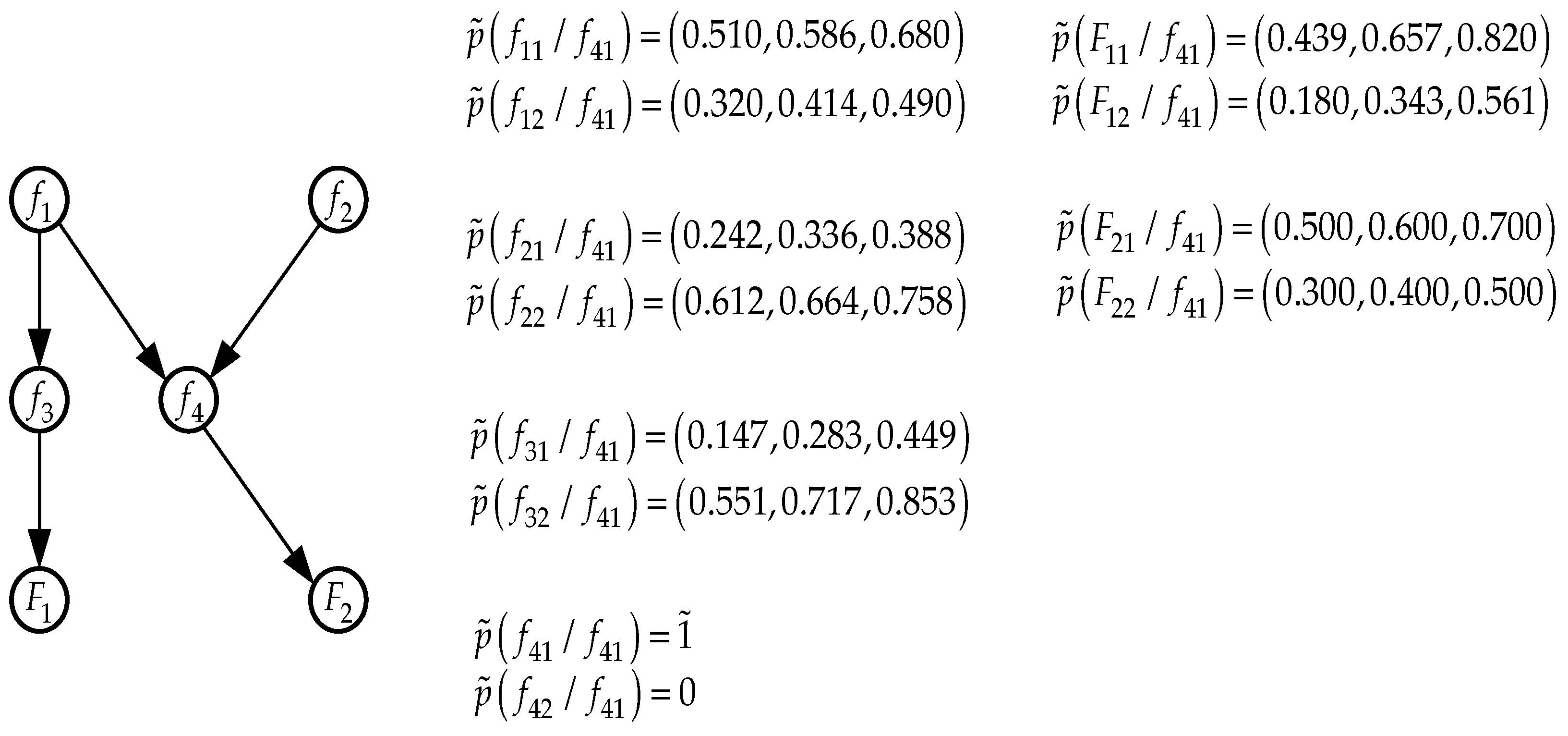
The reassigned fuzzy probability values are presented in Figure 8.
If the states of subfactors are realized sequentially in time in other nodes of the network, calculations of the full conditional probabilities are made by analogy, taking as the initial information obtained at the previous stage of the process and the fact of the implementation of a new state of one of the subfactors.
Based on the illustrative example presented above, the following scheme of algorithm actions can be established when propagating fuzzy posterior probabilities. When an event occurs in some intermediate node of the network (a specific state of the corresponding subfactor is realized), changes in the a priori fuzzy probabilities in the nodes of the branch (branches) from this node to the terminal node (to the terminal nodes) are happening due to changes in π ˜ -estimates. In Figure 8 this applies to nodes f 4 and F 2 . Changes in fuzzy prior probabilities in the branch (branches) to the initial node (to the initial nodes) of the network are happening due to changes in λ ˜ -estimates. In Figure 8 the change λ ˜ -estimates occur in the direction of the initial nodes f 1 and f 2 . In the branch (branches) from the initial node (nodes), in which no events occurred, the propagation of the influences of the event are happening due to changes in π ˜ -estimates (branch f 1 f 3 F 1 in Figure 8).
If an event (realization of a certain state of a specific subfactor) occurs at the initial node of the network, influences in the direction of terminal nodes are spread due to π ˜ -estimates. These influences propagate in the direction of other initial nodes due to changes in λ ˜ estimates. If there are other branches from other initial nodes, then in these branches the influences spread due to changes in π ˜ -estimates.

6. Discussion

In problems of assigning environmental risks, the determining factors probabilities are the probabilities of the occurrence of the states of the main factors since these states directly determine the adverse consequences. To analyze the results obtained in the illustrative example above, Table 1 presents the probabilities of factor states F 1 , F 2 for various states of the initial data.
From the data presented in this table, it follows that the implementation of the state f 41 of subfactor f 4 did not significantly affect the values full conditional posterior probabilities of factor F 1 states. But the values of the total posterior probabilities of the factor states F 2 have changed significantly. This is because the nodes F 2 and f 4 are connected by an arc on the Bayesian network graph. Therefore, the implementation of the subfactor state f 41 had as result such significant changes in the values of the total posterior probabilities p ˜ ( F 21 ) , p ˜ ( F 22 ) .
Let us present general conclusions, taking the material of this article as a basis. The Pearl algorithm allows us to formally solve the problem of probabilistic inference on a Bayesian network by calculating and propagating special λ ˜ -estimates and π ˜ -estimates along network arcs and calculating special λ ˜ -values and π ˜ -values in network nodes. But the original version of Pearl’s algorithm can only be used when the initial probabilistic estimates are given in deterministic form. In practice, in most cases, obtaining such estimates in tasks of assigning environmental risks seems unrealistic. It therefore seems appropriate to assign these estimates in an uncertain form. In this work, it is assumed that the initial estimates of all probabilities are given in the form of triangular normal fuzzy numbers.
To take advantage of Pearl’s algorithm when specifying probabilistic estimates in an uncertain form, in this article we proposed a fuzzy version of this algorithm. Based on the description of this fuzzy version in Section 4 and the results obtained in the illustrative example in Section 5, it can be confidently stated that the proposed version of the algorithm can be successfully used in the case of specifying relevant probability estimates in the form of triangular normal fuzzy numbers. The difference between the two versions of the algorithm lies only in the way the resulting estimates of the full conditional probabilities are normalized. In the original version of the algorithm, normalization of the resulting deterministic probability estimates is performed by simply dividing each probability estimate by the sum of all estimates. In the fuzzy version of the algorithm, normalization of the resulting fuzzy probabilistic estimates is performed in a more complex manner, using expressions (7)–(9). All other computational procedures in the proposed fuzzy version of the algorithm are performed by analogy with the procedures in the original version of the algorithm, only instead of point calculation estimates and values, their fuzzy analogues are used.

7. Materials and Methods

The material for research in this article are Bayesian networks that model complex multifactorial input data in problems of assigning environmental risks.
The study is based on the original version of the Pearl’s probability propagation algorithm on simply connected Bayesian networks. The article proposes a fuzzy version of this algorithm, based on which it is possible to solve problems of probabilistic inference on Bayesian networks that model the initial data in problems of assigning environmental risks with fuzzy initial probabilistic estimates.

8. Conclusions

The original version of Pearl’s algorithm works successfully when the probabilities of relevant events are specified in a crisp form. The current state of affairs in the field of environmental risk assignment indicates that it is more realistic to assign probabilistic estimates in an uncertain form, in particular, in the form of triangular fuzzy numbers.
The presented fuzzy version of the Pearl’s algorithm allows performing probabilistic inference on Bayesian networks in problems of assigning environmental risks when setting initial unconditional and conditional probability estimates in the form of triangular normal fuzzy numbers. It seems promising to offer versions of the algorithm for other types of fuzzy probability estimates, for example, in the form of interval-valued fuzzy numbers. The main requirement for such potentially possible versions of the algorithm is the availability of suitable approaches to normalizing probability estimates given in the appropriate fuzzy form.
In this paper, a fuzzy version of Pearl’s algorithm on arbitrary singly connected Bayesian networks is presented in the context of environmental risk assessment. This type of Bayesian networks is very common and is essentially an extension and generalization of tree-based and singly connected networks.
Much more difficult are the problems of abductive inference based on Pearl’s algorithm. Abductive inference is a process of reasoning that yields the best explanation (or some set of best explanations) under the conditions of a particular problem (Neapolitan 1990). It seems promising to develop fuzzy versions of Pearl’s algorithm for different types of abductive inference.
In this paper, a conditional environmental risk assignment problem is presented as an illustrative example of using the fuzzy version of the Pearl algorithm. Other problems where Bayesian networks and the fuzzy version of Pearl’s algorithm can be used include the following:
-
Representation of sets of states of the main factors of the emergence of a crisis situation in the economy and sets of states of subfactors related to each other and to the main factors;
-
Representation of sets of states of the main factors characterizing the possibility of an armed conflict between two states, and sets of states of subfactors related to each other and to the main factors;
-
Representation of sets of states of the main factors influencing the level of competitiveness of a large enterprise, and sets of states of subfactors related to each other and to the main factors.
The main advantage of the Pearl algorithm and its fuzzy version is that when any new state of any of the subfactors or the implementation of some combination of subfactor states is realized, a formal recalculation of the probabilities of the states of the main factors is performed. This allows management to continuously monitor a complex uncertain situation and, if necessary, make a timely and effective management decision.

Funding

This research received no external funding.

Institutional Review Board Statement

Not applicable.

Informed Consent Statement

Not applicable.

Data Availability Statement

The original contributions presented in the study are included in the article, further inquiries can be directed to the corresponding author.

Conflicts of Interest

The author declares no conflicts of interest.

References

  1. Adam, Vėronique, Alex von Wyl, and Bernd Novack. 2021. Probabilistic environmental risk assessment of micro- plastic in marine habitats. Aquatic Toxicology 230: 105689. [Google Scholar] [CrossRef] [PubMed]
  2. Alexander, David. 2013. Volcanic Ash in the Atmosphere and Risks for Civil Aviation: A Study in European Crisis management. International Journal Disaster Risk Science 4: 9–19. [Google Scholar] [CrossRef]
  3. Andrić, Jelena M., and Da-Gang Lu. 2017. Fuzzy probabilistic seismic hazard analysis with applications to Kumming city, China. Natural Hazards 89: 1–27. [Google Scholar] [CrossRef]
  4. Ansari, Zakir Ali, and S. G. Prabhu Matondkar. 2014. Anthropogenic Activities Including Pollution and Contamination of Coastal Marine Environment. Journal of Ecophysiology and Occupational Health 14: 71–78. [Google Scholar] [CrossRef]
  5. Arihilam, Ngozi, and E. Arihilam. 2019. Impact and control of anthropogenic pollution on the ecosystem—A review. Journal of Bioscience and Biotechnology Discovery 4: 54–79. [Google Scholar] [CrossRef]
  6. Baker, Jack W., Brendon A. Bradley, and Peter J. Stafford. 2021. Seismic Hazard and Risk Analysis. Cambridge: Cambridge University Press. [Google Scholar]
  7. Behrens, Jörn, Finn Løvholt, Fatemeh Jalayer, Stefano Lorito, Mario A. Salgado-Gálvez, Mathilde Sørensen, Stephane Abadie, Ignacio Aguirre-Ayerbe, Iñigo Aniel-Quiroga, Andrey Babeyko, and et al. 2021. Probabilistic Tsunami Hazard and Risk Analysis: A Review. Frontiers in Earth Science 9: 628772. [Google Scholar] [CrossRef]
  8. Belza, Concha, and Pedro Larrañaga. 2014. Bayesian networks in neuroscience: A survey. Frontiers in Computational Neuroscience 8: 131. [Google Scholar] [CrossRef]
  9. Boc, Kamil, Jurai Vasilík, and Dagmar Vidriková. 2012. Fuzzy Approach to Risk Analysis and its Advantages Against the Qualitative Approach. Paper presented at 12th Conference “Reliability and Statistic in Transportation and Communication”, Riga, Latvia, October 17–20. [Google Scholar]
  10. Bommer, Julian. 2021. Review of Seismic Hazard and Risk Analysis. Seismological Research Letters 92: 3248–50. [Google Scholar] [CrossRef]
  11. Booth, Adam, Angus Bruno Reed, Sonia Ponzo, Arrash Yassaee, Mert Aral, David Plans, Alain Labrique, and Diwakar Mohan. 2021. Poulation risk factors for severe disease and mortality in COVID-19: A global systematic review and metaanalysis. PLoS ONE 16: e0247461. [Google Scholar] [CrossRef]
  12. Borisov, Vadim Vladimirovich, Sergei A. Ponomarenko, Alexander Sergeevich Fedulov, and Vladimir I. Bobkov. 2019. Complex system risk assessment based on the fuzzy probabilistic Bayesian inference. ATP Conference Proceedings 2176: 040003. [Google Scholar] [CrossRef]
  13. Castillo, Enrique, Josė M. Gutėrrez, and Ali S. Hadi. 1997. Expert Systems and Probabilistic Network Models. New York: Springer. [Google Scholar]
  14. De Campos, Luis M., Juan F. Huete, and Serafin Moral. 1994. Probability Intervals: A Tool for Uncertain Reasoning. International Journal of Uncertainty, Fuzziness and Knowledge-Based Systems 2: 167–96. [Google Scholar] [CrossRef]
  15. Dickey, James W. E., Ross N. Guthbert, Michael Rea, Ciaran Laverty, Kate Crane, Josie South, Elizabeta Driski, Xiexiu Chang, Neil E. Coughlan, Hugh J. Macissac, and et al. 2018. Assessing the relative ecological impact and invasion risks of emerging and future invasive alien species. Neo Biota 40: 1–24. [Google Scholar] [CrossRef]
  16. Erdem, Fatma. 2022. Risk assessment with the fuzzy logic method for Ankara OIZ environmental waste water treatment plant. Turkish Journal of Engineering 6: 268–75. [Google Scholar] [CrossRef]
  17. Favaretto, Paula. 2024. Modeling Lung Cancer Diagnosis Using Bayesian Network Inference. Available online: https://www.mathworks.com/matlabcentral/fileexchange/17862-modeling-lung-cancer-diagnosis-using-bayesian-network-inference (accessed on 22 April 2024).
  18. Ghomshei, Mory M., and John A. Meech. 2010. Application of Fuzzy Logic in Environmental Risk Assessment: Some Thoughts on Fuzzy Sets. Cybernetics and Systems 31: 317–52. [Google Scholar] [CrossRef]
  19. Grieser, Jürgen, and Phil Heines. 2020. Tornado Risk Climatology in Europe. Atmosphere 11: 768. [Google Scholar] [CrossRef]
  20. Hong, Hyunjoo, Vėronique Adam, and Bernd Novack. 2021. Form-Specific and Probabilistic Environmental Risk Assessment of 3 Engineered Nanomaterials (Nano-Ag, Nano TiO2, and ZnO) in European Freshwaters. Environmental Toxicology and Chemistry 40: 2629–39. [Google Scholar] [CrossRef]
  21. Iderawumi, Addulraheem M. 2019. Sources of Environment Hazards Effects and Control. Asia Pacific Journal of Energy and Environment 6: 77–82. [Google Scholar] [CrossRef]
  22. Jensen, Finn V., and Thomas D. Nielsen. 2007. Networks and Decision Graphs, 2nd ed. Berlin/Heidelberg: Springer. [Google Scholar]
  23. Jordan, Michael I. 1997. An Introduction to Graphical Models. Center for Biological and Computational Learning. Massachusetts Institute of Technology. Available online: https://docslib.org/doc/11226934/an-introduction-to-graphical-models (accessed on 10 March 2024).
  24. Ketsap, Akkachai, Hansapinuo Chqyanon, Kronparset Nopaden, and Limkatanyu Suchart. 2019. Uncertainty and Fuzzy Decision in Earthquake risk Evaluation of Building. Engineering Journal 23: 89–105. [Google Scholar] [CrossRef]
  25. Korb, Kevin D., and Ann E. Nicholson. 2011. Bayesian Artificial Intelligence, 2nd ed. Boca Raton: Chapman & Hall. [Google Scholar]
  26. Kumar, Rai P., and J. S. Singh. 2020. Invasive alien plant species: Their impact on environment, ecosystem services and human health. Ecological Indicators 111: 106020. [Google Scholar] [CrossRef]
  27. Lauritzen, Steffen L. 2020. Lectures on Graphical Models, 3rd ed. København: University of Copenhagen, Department of Mathematical Sciences. [Google Scholar]
  28. Linders, Teo Edmund Werner, Urs Schaffner, Renė Eschen, Anteneh Adebe, Simon Kevin Choge, Lisanework Nigafu, Purity Rima Nbaabu, Kailu Shieraw, and Eric Allan. 2019. Direct and indirect effects of invasive species: Biodiversity loss in a major mechanism by with an invasive tree effects ecosystem functioning. Journal of Ecology 107: 2660–72. [Google Scholar] [CrossRef]
  29. Liu, Guilin, Jingyi Yin, Shichun Song, Wenjin Yang, Yuhang Tian, Liping Wang, and Yu Xu. 2023. Risk Estimation of Typhon Disaster Based on Three-Dimensional Information Diffusion Method. Journal of Marine Science and Engineering 11: 1080. [Google Scholar] [CrossRef]
  30. Maertens, Alexandra, Emily Golden, Thomas H. Luechtefeld, Sebastian Hoffmann, Katya Tsaioun, and Thomas Hartung. 2022. Probabilistic risk assessment—The keystone for the future of toxicology. ALTEX 39: 3–29. [Google Scholar] [CrossRef]
  31. Mentzel, Sophie, Merete Grung, Knut E. Telletsen, Marianne Stenrød, Karina Petersen, and S. Janicke Moe. 2022. Development of a Bayesian network for probabilistic risk assessment of pesticides. Integrated Environmental Assessment and Management 18: 1072–87. [Google Scholar] [CrossRef]
  32. Nastos, Panagiotis T., Nicolas R. Dalezios, Joannis N. Faraslis, Kostas Mitrokopoulos, Anna Blanta, Marios Spilietopolus, Stavros Sakellariouos, Pantelis Sidirooulos, and Ana M. Tarquis. 2021. Review article: Risk management framework of environmental hazard and extremes in Mediterranean ecosystems. Natural Hazards and Earth System Sciences 21: 1935–54. [Google Scholar] [CrossRef]
  33. Neapolitan, Richard E. 1990. Probabilistic Reasoning in Expert Systems. Theory and Algorithms. Hoboken: John Wiley & Sons. [Google Scholar]
  34. Neapolitan, Richard E. 2004. Learning Bayesian Networks. Hoboken: Pearson Prentice Hall. [Google Scholar]
  35. Oberdorfer, Stefan, Philip Sander, and Sven Fuchs. 2020. Multi-hazard risk assessment for risk: Probabilistic versus deterministic approach. Natural Hazards and Earth System Sciences 20: 3135–60. [Google Scholar] [CrossRef]
  36. Pearl, Judea. 1988. Probabilistic Reasoning in Intelligent Systems. San Mateo: Morgan Kaufman. [Google Scholar]
  37. Prűss-Ustűn, Annette, Jennyfer Wolf, Carlos S. Corvalán, Robert Bos, and Maria P. Neira. 2016. Preventing Disease through Healthy Environments: A Global Assessment of the Burden of Disease from Environmental Risks. Geneva: World Health Organization. Available online: https://iris.who.int/handle/10665/204585 (accessed on 5 November 2023).
  38. Raadgever, G. T., Nikėh Booister, and Martin Steens. 2018. Flood Risk Management Strategies. In Flood Risk Management Strategies and Governance. Berlin/Heidelberg: Springer, pp. 93–100. [Google Scholar] [CrossRef]
  39. Radionovs, Andrejs, and Oleg Uzhga-Rebrov. 2014. Application of Fuzzy Logic for Risk Assessment. Information Technology and Management Science 17: 50–54. [Google Scholar] [CrossRef]
  40. Reynolds, Sam A., and David C. Aldridge. 2021. Global impacts of invasive species on the tipping points of shallow lakes. Global Change Biology 23: 6129–38. [Google Scholar] [CrossRef]
  41. Rhind, S. M. 2009. Anthropogenic pollutants: A threat to ecosystem sustainability? Philosophical Transactions of the Royal Society B 364: 3391–401. [Google Scholar] [CrossRef] [PubMed]
  42. Roisenberg, Mauro, Sintia Shoeninger, and Reneu da Silva. 2009. A hybrid fuzzy-probabilistic system for risk analysis in petroleum exploration projects. Expert Systems and Applications 36: 6282–94. [Google Scholar] [CrossRef]
  43. Rojas-Rueda, David, Emily Morales-Zamora, Wael Abdullah Alsufyani, Christopher H. Herbst, Salem M. AlBalawi, Reem Alsukait, and Mashael Alomran. 2021. Environmental Risk Factors and Health” An Umbrella Review of Meta-Analyses. International Journal of Environmental Research and Public Health 18: 704. [Google Scholar] [CrossRef]
  44. Sari, A. M., and A. Fakhrurrozi. 2018. Earthquake Hazard Analysis Methods: A Review. IOP Conference Series: Earth and Environmental Science 118: 012044. [Google Scholar] [CrossRef]
  45. Soltanzadeh, Ahmad, Mahdinia Mohsen, and Mohammadfam Iraj. 2022. Fuzzy Logic-based Risk Analysis of COVID-19 Infection: A Case Study in Healthcare Facilities. Health in Emergencies and Disasters Quarterly 8: 55–64. [Google Scholar] [CrossRef]
  46. Stephenson, Told A. 2000. An Introduction to Bayesian Network. Theory and Usage. IDIAP Research Report 00-03. Martigny: IDIAP. [Google Scholar]
  47. Uzhga-Rebrov, Oleg. 2016. Uncertainty Management. Part 4. Combining Uncertainties. Rezekne: RA Publishing House. (In Russian) [Google Scholar]
  48. Uzhga-Rebrov, Oleg. 2019. Estimation, Analysis and Propagation of Uncertainties. Rezekne: RA Drukatava. 582p. (In Russian) [Google Scholar]
Figure 1. Main types of connections between nodes on a Bayesian network. (a) chain connection, (b) divergent type of connections, (c) convergent type of connections.
Risks 12 00135 g001
Figure 2. Characteristic types of Bayesian network structures. (a) tree-like Bayesian network, (b) simply connected Bayesian network.
Risks 12 00135 g002
Figure 3. Common types of probabilistic inference (reasoning) on Bayesian networks. (a) diagnostic inference, (b) predictive inference, (c) intercausal inference, (d) combined inference. S—patient is smoker; D—patient has a dyspnea; P—patient has a pollution; X-ray.
Risks 12 00135 g003
Figure 4. Possible types of Bayesian networks in problems of probabilistic risk assignment. (a) tree-like connections between subfactors and factors, (b) the convergent-divergent type of connections between subfactors and factors, (c) the chain-convergent type of connections between subfactirs and factors.
Risks 12 00135 g004
Figure 5. Fragment of a conditional Bayesian network.
Risks 12 00135 g005
Figure 6. Simply connected Bayesian network and initial fuzzy assignments of unconditional and conditional probabilities of states of subfactors and factors in network nodes.
Risks 12 00135 g006
Figure 7. Bayesian network from Figure 6 and the values of complete a priori fuzzy conditional probabilities in network nodes.
Risks 12 00135 g007
Figure 8. Fuzzy probability values in network nodes after in the node f 4 has implemented a state f 41 .
Risks 12 00135 g008
Table 1. Probability values of factor states F 1 , F 2 for various states of initial data.
Events (States of Factors)Full Conditional
Prior Probabilities
Full Conditional
Posterior Probabilities
F 11 (0.440, 0.664, 0.821)(0.439, 0.657, 0.820)
F 12 (0.168, 336, 0.560)(0.180, 0.343, 0.561)
F 21 (0.143, 0.369, 0.457)(0.500, 0.600, 0.700)
F 22 (0.543, 0.631, 0.857)(0.300, 0.400, 0.500)
Disclaimer/Publisher’s Note: The statements, opinions and data contained in all publications are solely those of the individual author(s) and contributor(s) and not of MDPI and/or the editor(s). MDPI and/or the editor(s) disclaim responsibility for any injury to people or property resulting from any ideas, methods, instructions or products referred to in the content.