Pricing Life Contingencies Linked to Impaired Life Expectancies Using Intuitionistic Fuzzy Parameters

Abstract

Several life contingency agreements are based on the assumption that policyholders have impaired life expectancy attributable to factors, such as lifestyle, social class, or preexisting health issues. Quantifying two crucial variables, augmented death probabilities and the discount rate of projected cash flows, is essential for pricing such agreements. Information regarding the correct values of these parameters is subject to vagueness and imprecision, which further intensifies if impairments must be considered. This study proposes modelling mortality and interest rates using a generalization of fuzzy numbers (FNs), known as intuitionistic fuzzy numbers (IFNs). Consequently, this paper extends the literature on life contingency pricing with fuzzy parameters, where uncertainty in variables, such as interest rates and death probabilities, is modelled using FNs. While FNs introduce epistemic uncertainty, the use of IFNs adds bipolarity to the analysis by incorporating both positive and negative information regarding actuarial variables. Our analysis focuses on two agreements involving policyholders with impaired life expectancies: determining the annuity payment in a substandard annuity and pricing a life settlement over a whole life insurance policy. In particular, we emphasize modelling interest rates and survival probabilities using triangular intuitionistic fuzzy numbers (TIFNs) owing to their ease of interpretation and implementation.

1. Introduction

Life insurers have traditionally focused on providing standardized life coverages, pricing them primarily based on age and, when permissible, gender (Gatzert and Klotzki 2016). However, since the last few decades of the 20th century, a significant trend in the insurance industry has been the customization of services to align with the individual needs of the insured (Sosa and Montes 2022). This shift underscores the importance of considering the heterogeneity of life expectancies in the offering and valuation of policies addressing life contingencies, such as life annuities (Olivieri and Pitacco 2016).

Within the realm of life contingency insurance, two general types can be distinguished: life annuities, covering the contingency of survival, and life insurance, addressing the contingency of death (Promislow 2014). In both types of insurance contracts, there are agreements in which projected cash flows are established to individualize the mortality of insured persons. This approach involves considering the possibility that owing to their particular lifestyle, health, etc., an insured person may have a diminished life expectancy (LE) compared to the expected norm for their age. This study addresses two situations in actuarial pricing linked to life contingencies associated with life insurance coverage: special-rate life annuities and life settlements.

In the domain of life annuities, the use of standard probabilities for evaluation is attractive, primarily for healthy individuals, but may not be suitable for those with impaired life expectancy. Thus, to expand their market, some insurers offer elevated annuity rates to individuals with critical health conditions (Olivieri and Pitacco 2016). This practice is known as a special rate or substandard annuity.

When a policyholder seeks to liquidate life insurance prematurely, the insurer determines the amount offered, referred to as the surrender value, by valuing it using standard death probabilities. In highly developed life markets, such as those of the United States, there is the option to sell life insurance to third parties—investors in life insurance policies—under agreements known as life settlements (LSs). Through these transactions, policyholders with impaired life expectancies can obtain greater value by selling their policies than the surrender value (Brockett et al. 2013) because reduced LEs are associated with higher prices. This is because of the likelihood that investors will pay fewer pending insurance premiums, and the death benefit is expected sooner (Braun and Xu 2020).

The assessment of life contingencies with heterogeneous life expectancies (LEs) relies on conventional life insurance mathematics, involving the discounted value of expected cash flows with an appropriate interest rate and death probabilities tailored to the specific policyholder. This approach applies to both special-rate annuities (Pitacco 2017) and life settlements (LSs) (Braun and Xu 2020). Adjusting one-year death probabilities suited to the policy of interest is typically performed by referencing a standard mortality law corresponding to a large group, representing the mortality behavior of an “average” person and subsequently adapting it to the particular characteristics of the life contingencies intended for valuation (Olivieri 2006).

The parameters embedded in life insurance pricing are subject to various types of uncertainty, such as risk, vagueness, and imprecision. Traditionally, the valuation of life contingencies has operated under the assumption of pure risk, wherein the probabilities associated with potential outcomes (e.g., death, survival, or disability) are considered to be perfectly known. Consequently, the discounted valuation of cash flows typically assumes that the parameters associated with valuation, primarily interest rate and survival probabilities, are quantifiable by real numbers. This holds true for standard life contingencies (Promislow 2014), special-rate annuities (Pitacco 2017), and life settlements (Lubovich et al. 2008).

However, in practice, information regarding the precise values of parameters used in life contingency valuation contains various sources of imprecision and uncertainty; thus, employing crisp parameters represents a simplification (Lemaire 1990). The technical interest rate paid by insurance companies to policyholders and annuitants must align with the risk-free interest rate expected in the economy over the duration of the contract. This requires making prudent assumptions about the risk-free interest rate in the long term, the knowledge of which is inherently vague (Devolder 1988).

Uncertainty also significantly influences the standard mortality probabilities used in valuation given that the evolution of population mortality over time is not predictable with absolute precision. To address this, dynamic stochastic mortality models have been developed, for example, as described by Lee and Carter (1992). Moreover, considering heterogeneous life expectancies introduces additional sources of uncertainty into mortality probabilities. Many factors influencing life expectancy are inherently imprecise from a medical standpoint (Anderton and Robb 1998), and policyholders often possess more information about their LEs than evaluators do (Bauer et al. 2020). Furthermore, information provided by applicants in medical interviews may be inaccurate, false, or incomplete, often because they have incentives to obtain more favorable prices (Bundock 2006). Additionally, ongoing advancements in medical technologies have contributed to increasing life expectancies, potentially surpassing the estimates made at the time of valuation based on available information (Xu and Hoesch 2018).

Fuzzy set theory (FST) provides tools, such as fuzzy expert systems, fuzzy numbers, fuzzy random variables, and fuzzy regression, allowing for the treatment of uncertainty. These tools have been in use since the 1980s in financial and actuarial mathematics. While traditional financial methods, such as cash flow discount models or option pricing models, provide a solid analytical foundation, the integration of fuzzy tools can improve the results by addressing additional sources of uncertainty alongside inherent risks (Andrés-Sánchez 2023).

In the realm of financial and actuarial pricing, seminal works by Kaufmann (1986), Buckley (1987), and Lemaire (1990) proposed modelling uncertain parameters using fuzzy numbers (FNs). In these contributions, FNs must be interpreted as quantifications of epistemic uncertainty, capturing vague or incomplete information about the value of the parameter of interest (Dubois and Prade 2012). Let $\rho$ be a variable (the adequate discount rate). We can define the fuzzy number $\hat{\rho }$, interpreted as “the discount rate must be approximately $\hat{\rho }$,” by using a possibility distribution that measures the ease with which a value $x$ is equal to $\rho$. This interpretation of an FN has been widely used in FSTs for financial and actuarial analyses.

Following Dong and Li (2016), capital budgeting and cash-flow discounting were the initial domains in which uncertainty was introduced by means of fuzzy numbers. This includes the computation of the net present value (Kaufmann 1986), the internal rate of return (IRR) (Buckley 1992), and the terminal value of an investment project (Kahraman et al. 2002). Likewise, the application of a fuzzy-random approach to option pricing, both in continuous time and discrete time, has been a burgeoning field in this regard (Muzzioli and De Baets 2016; Andrés-Sánchez 2023).

Although FST is far from being at the core of actuarial science, Table 1 shows that various authors have found that its application could be useful in different actuarial areas. These studies have been published in both applied mathematics journals and more specialized actuarial mathematics journals. Notably, there is a specific chapter dedicated to fuzzy sets in the Encyclopedia of Actuarial Science (Derrig and Ostaszewski 2006).

Table 1. Contributions to the financial–actuarial valuation of the arithmetic of fuzzy numbers.

Issue	Papers
Life insurance pricing (cash-flow discounting)	Lemaire (1990), Ostaszewski (1993), Andrés-Sánchez and Terceño (2003), Shapiro (2004), Andrés Sánchez and González-Vila (2012, 2017a, 2017b, 2023), Andrés-Sánchez et al. (2020), Aalaei (2022), Dębicka et al. (2022).
Life insurance pricing (final value)	Cassú et al. (1996), Betzuen et al. (1997),
Insurance pricing (option pricing)	Xu et al. (2009), Anzilli and Facchinetti (2017), Nowak and Romaniuk (2017), Anzilli et al. (2018).
Nonlife insurance (cash-flow discounting)	Derrig and Ostaszewski (1997), Cummins and Derrig (1997), Andrés-Sánchez and Terceño (2003), Andrés-Sánchez (2014),
Nonlife insurance (terminal value)	Mircea and Covrig (2015), Ungureanu and Vernic (2015),
Claim reserving	Andrés-Sánchez and Terceño (2003), Apaydin and Baser (2010), Andrés-Sánchez (2012), Heberle and Thomas (2014), Heberle and Thomas (2016), Woundjiagué et al. (2019).

Fuzzy actuarial pricing, in both life insurance (Lemaire 1990) and nonlife insurance (Cummins and Derrig 1997), primarily involves using the discounted value of projected cash flows. However, in the field of life contingency analysis, Anzilli and Facchinetti (2017), Nowak and Romaniuk (2017), and Anzilli et al. (2018) applied option pricing methods with fuzzy parameters. Similarly, Mircea and Covrig (2015) and Ungureanu and Vernic (2015) model the terminal value of an insurance company within a predefined time horizon as the terminal value of its projected cash flows. In the nonlife insurance sector, Apaydin and Baser (2010) and Heberle and Thomas (2014) explore the development of fuzzy claim reserving.

The concept of intuitionistic fuzzy numbers (IFNs) is a tool in the theory of intuitionistic fuzzy sets presented by Atanassov (1986) and Atanassov (1989) that allows for the quantification of uncertain quantities. They extend the concept of FNs (Mitchell 2004) and facilitate the inclusion of bipolar information along with epistemic uncertainty in the quantification of parameters of interest. In this context, bipolarity involves considering both positive information regarding the potential values of the parameter of interest and negative information related to the values that the parameter actually cannot take (Dubois and Prade 2012).

According to Dubois and Prade (2012), the bipolarity considered in instruments such as IFNs does not introduce additional uncertainty; however, it does provide new information. In the case of IFNs, this entails adding an estimate of values that, with certainty, should be excluded, thus complementing information about the believed possible values of a quantity.

The application of IFN parameters in financial pricing is significantly scarcer than that of conventional fuzzy numbers, especially in finance, and is absent in actuarial pricing. The relevant applications include capital budgeting (Kumar and Bajaj 2014; Kahraman et al. 2015; Boltürk and Kahraman 2022; Haktanır and Kahraman 2023), option pricing (Wu et al. 2016), and real option pricing (Ersen et al. 2018; Ersen et al. 2023).

Building upon the reflections presented in the introduction, this study expands upon the findings of Andrés-Sánchez et al. (2020) on special-rate annuities and Aalaei (2022) and Andrés-Sánchez and González-Vila (2023) on LSs. These contributions model the uncertainty of LE and adequate discount rates using FNs. This work generalizes these results by considering that information about these parameters is provided by IFNs, with a specific focus on triangular IFNs owing to their greater practical applicability.

The remainder of this paper is organized as follows. The next section introduces the fundamentals of intuitionistic fuzzy numbers and their arithmetic operations. The third section develops elements of life insurance in the presence of heterogeneity in LEs under the hypothesis that discount and mortality rates are estimated by means of IFNs. The fourth section develops substandard life annuities and life-settlement pricing in the presence of intuitionistic information. We compare the results of the numerical applications with those obtained by modelling uncertain parameters with equivalent random variables following Dubois et al. (2004). The study concludes by highlighting the main results and suggesting further research.

2. Intuitionistic Fuzzy Numbers

2.1. Fuzzy Numbers and Intuitionistic Fuzzy Numbers

Definition 1. 

A fuzzy set (FS) in a referential set $X$, $\widehat{A}$ is defined as (Zadeh 1965):

$$\widehat{A}=\left\{⟨x,{\mu }_A\left(x\right)⟩, x\in X\right\},$$

where ${\mu }_A:X⟶\left[0,1\right]$ is the so-called membership function.

Definition 2. 

The fuzzy set $\widehat{A}$ can be represented through level sets or $\alpha$-cuts, $A_{\alpha }$ (Zadeh 1965):

$$A_{\alpha }=\left\{x|{\mu }_A\left(x\right)\ge \alpha , 0<\alpha \le 1\right\}.$$

Definition 3. 

A fuzzy number (FN), $\widehat{A}$, is a fuzzy subset of the real line (Dubois and Prade 1993), such that

i. 

is normal, i.e.,  $\exists x|{\mu }_A\left(x\right)=1.$

ii. 

is convex, i.e.,

$$\forall x_1,x_2\in \mathbb{R},0\le \lambda \le 1,{\mu }_A\left({\lambda x}_1,\left(1-\lambda \right)x_2\right)\ge \min \left({\mu }_A\left(x_1\right),{\mu }_A\left(x_2\right)\right).$$

Remark 1. 

As a consequence, the α-cuts of $\widehat{A}$, $A_{\alpha }$ are confidence intervals:

$$A_{\alpha }=\left\{x|{\mu }_A\left(x\right)\ge \alpha , 0<\alpha \le 1\right\}=\left[{\underset{\_}{A}}_{\alpha }, {\overline{A}}_{\alpha }\right],$$

 where ${\underset{\_}{A}}_{\alpha }$ is an increasing function of $\alpha$ and ${\overline{A}}_{\alpha }$ is a decreasing function.

Fuzzy set theory commonly represents imprecise quantities and parameters using fuzzy numbers (FNs) (Dubois and Prade 1993).

Definition 4. 

A triangular fuzzy number (TFN) can be represented by the triplet $\widehat{A}=\left(A^{\left(l\right)},A^{\left(c\right)},A^{\left(r\right)}\right)$, $A^{\left(l\right)}\le A^{\left(c\right)}\le A^{\left(r\right)}$:

$${\mu }_A\left(x\right)=\left\{\begin{array}{cc}\frac{x-A^{\left(l\right)}}{A^{\left(c\right)}-A^{\left(l\right)}}& A^{\left(l\right)}\le x\le A^{\left(c\right)}\\ \frac{A^{\left(r\right)}-x}{A^{\left(r\right)}-A^{\left(c\right)}}& A^{\left(c\right)}\le x\le A^{\left(r\right)}\\ 0& \mathrm{o}\mathrm{t}\mathrm{h}\mathrm{e}\mathrm{r}\mathrm{w}\mathrm{i}\mathrm{s}\mathrm{e}\end{array}\right.,$$

and its α-cut representation:

$$A_{\alpha }=\left[{\underset{\_}{A}}_{\alpha }, {\overline{A}}_{\alpha }\right]=\left[A^{\left(l\right)}+\left(A^{\left(c\right)}-A^{\left(l\right)}\right)\alpha ,{ A}^{\left(r\right)}-\left(A^{\left(r\right)}-A^{\left(c\right)}\right)\alpha \right], 0\le \alpha \le 1.$$

Within fuzzy set theory, TFNs are very common in practical financial applications (Andrés-Sánchez 2023). In triangular fuzzy numbers, the grading of the membership level is performed linearly, which is reasonable because it applies the principle of parsimony when dealing with vague information (Jiménez and Rivas 1998).

Thus, the fuzzy number $\tilde{A}$ is interpreted as a value that is approximately $A^{\left(c\right)}$ with the lower and upper extreme scenarios denoted as $A^{\left(l\right)}$ and $A^{\left(r\right)}$, respectively. For example, an economic prediction such as “the inflation next year will be approximately 3%, and we do not expect it to be below 2.5% or above 4%” can be represented as (2.5%, 3%, 4%).

Definition 5. 

The intuitionistic fuzzy set (IFS) $\tilde{A}$ defined in a referential set $X$ is (Atanassov 1986):

$$\tilde{A}=\left\{⟨x,{\mu }_A\left(x\right),v_A\left(x\right)⟩, x\in X\right\},$$

where ${\mu }_A:X⟶\left[0,1\right]$ measures the membership of $x$ in $\tilde{A}$ and $v_A:X⟶\left[0,1\right]$ is nonmembership. The corresponding functions are as follows:

$$0\le {\mu }_A\left(x\right)+v_A\left(x\right)\le 1.$$

Remark 2. 

Note that not necessarily ${\mu }_A\left(x\right)+v_A\left(x\right)=1$; that is, an element $x$ is allowed to avoid belonging to $\tilde{A}$ and its complement with a degree of hesitancy, $h_A\left(x\right)$, which is:

$$h_A\left(x\right)=1-{\mu }_A\left(x\right)-v_A\left(x\right).$$

Remark 3. 

The IFSs generalize the concept of an FS, such that if $h_A\left(x\right)=0 \forall x$, $\tilde{A}$ is a conventional FS $\widehat{A}$.

Definition 6. 

An IFN can be expressed using $⟨\alpha ,\beta ⟩$-levels or $⟨\alpha ,\beta ⟩$-cuts, $A_{⟨\alpha ,\beta ⟩}$ (Atanassov 1986):

$$A_{⟨\alpha ,\beta ⟩}=\left\{x|{\mu }_A\left(x\right)\ge \alpha , v_A\left(x\right)\le \beta ,0\le \alpha +\beta \le 1,\alpha ,\beta \in \left[0,1\right]\right\}.$$

Remark 4. 

$A_{⟨\alpha ,\beta ⟩}$ can be decoupled into two level sets (Yuan et al. 2014):

$$A_{\alpha }=\left\{{x|\mu }_A\left(x\right)\ge \alpha \right\} \mathrm{a}\mathrm{n}\mathrm{d} A_{\beta }^{*}=\left\{x|v_A\left(x\right)\le \beta \right\},$$

in such a way that

$$A_{⟨\alpha ,\mathsf{\beta }⟩}=⟨A_{\alpha }=\left\{{x|\mu }_A\left(x\right)\ge \alpha \right\},A_{\beta }^{*}=\left\{x|v_A\left(x\right)\le \beta \right\},0\le \mathsf{\alpha }+\beta \le 1,\mathsf{\alpha },\beta \in \left[0,1\right]⟩.$$

Definition 7. 

A fuzzy subset ${\widehat{A}}^{*}$ is considered. Following Burillo and Bustince (1996), IFS can be induced by means of an application $\Phi :FSs\to IFSs,$ $\tilde{A}=\Phi \left({\widehat{A}}^{*}\right)$ by stating ${\alpha }_x$ and $h_{A^{*}}\left(x\right)$ as follows:

i. 

${\alpha }_x\ge {\mu }_{A^{*}}\left(x\right)$,

ii. 

$h_{A^{*}}\left(x\right)\le \frac{{\mu }_{A^{*}}\left(x\right)}{{\alpha }_x}$

and then:

$$\begin{array}{l}{\mu }_A\left(x\right)={\mu }_{A^{*}}\left(x\right)-{\alpha }_x{h}_{A^{*}}\left(x\right),\\ v_A\left(x\right)=1-{\mu }_{A^{*}}\left(x\right)+{\alpha }_x{h}_{A^{*}}\left(x\right)-h_{A^{*}}\left(x\right),\\ h_A\left(x\right)=h_{A^{*}}\left(x\right).\end{array}$$

Definition 8. 

An intuitionistic fuzzy number (IFN) is an IFS defined on real numbers (Kahraman et al. 2015), such that

i. 

It is normal, i.e., $\exists x|{\mu }_A\left(x\right)=1\Rightarrow v_A\left(x\right)=h_A\left(x\right)=0.$

ii. 

${\mu }_A\left(x\right)$ is convex,

$$\forall x_1,x_2\in \mathbb{R},0\le \lambda \le 1,{\mu }_A\left({\lambda x}_1,\left(1-\lambda \right)x_2\right)\ge \min \left({\mu }_A\left(x_1\right),{\mu }_A\left(x_2\right)\right),$$

iii. 

and $v_A\left(x\right)$ is concave:

$$\forall x_1,x_2\in \mathbb{R},0\le \lambda \le 1,v_A\left({\lambda x}_1,\left(1-\lambda \right)x_2\right)\le \max \left(v_A\left(x_1\right),v_A\left(x_2\right)\right).$$

Remark 5. 

The $⟨\alpha ,\beta ⟩$-cuts of $\tilde{A}$ and $A_{⟨\alpha ,\beta ⟩}$ can be decoupled as:

$$A_{\alpha }=\left\{{x|\mu }_A\left(x\right)\ge \alpha \right\}=\left[{\underset{\_}{A}}_{\alpha },{\overline{A}}_{\alpha }\right] \mathrm{a}\mathrm{n}\mathrm{d} A_{\beta }^{*}=\left\{v_A\left(x\right)\le \beta \right\}=\left[{\underset{\_}{A^{*}}}_{\beta },{\overline{A^{*}}}_{\beta }\right],0\le \mathsf{\alpha }+\beta \le 1,\mathsf{\alpha },\beta \in (0,1),$$

where ${\underset{\_}{A}}_{\alpha }$ $\left({\overline{A}}_{\alpha }\right)$is an increasing (decreasing) function of $\alpha$ and ${\underset{\_}{A^{*}}}_{\beta }$ $\left({\overline{A^{*}}}_{\beta }\right)$ decreases (increases) with respect to $\beta$.

Remark 6. 

Thus, an $⟨\alpha ,\beta ⟩$-level of $A_{⟨\alpha ,\beta ⟩}$ can be represented:

$$A_{⟨\alpha ,\beta ⟩}=⟨A_{\alpha }=\left[{\underset{\_}{A}}_{\alpha },{\overline{A}}_{\alpha }\right],{A^{*}}_{\beta }=\left[{\underset{\_}{A^{*}}}_{\beta },{\overline{A^{*}}}_{\beta }\right],0\le \alpha +\beta \le 1,\mathsf{\alpha },\beta \in (0,1)⟩.$$

An IFN is an imprecise quantity that is measured using a real number. If nonmembership is established as $v_A\left(x\right)=1-{\mu }_A\left(x\right) \forall x$, then $\tilde{A}$ is an FN.

Remark 7. 

FN ${\widehat{A}}^{*}$ generates an IFN $\tilde{A}$ by considering Definition 7 ${\alpha }_x=1$. Therefore, in this case, ${\mu }_A\left(x\right)={\mu }_{A^{*}}\left(x\right)-h_A\left(x\right)$ and $v_A\left(x\right)=1-{\mu }_{A^{*}}\left(x\right)$.

Following Mitchell (2004), ${\mu }_{A^{*}}\left(x\right)=1-v_A\left(x\right)$ can be interpreted as the upper distribution function of the uncertain quantity $A$, and ${\mu }_A\left(x\right)$ can be interpreted as the lower distribution function. In this way, Dubois and Prade (2012) interpreted ${\mu }_{A^{*}}\left(x\right)$ and ${\mu }_A\left(x\right)$ as bipolar possibility distribution measurements in such a way that ${\mu }_{A^{*}}\left(x\right)$ accounts for the potential possibility and ${\mu }_A\left(x\right)$ accounts for the real possibility of $A$ being $x$.

Definition 9. 

A triangular intuitionistic fuzzy number (TIFN) $\tilde{A}$ can be denoted as $\tilde{A}=⟨\left(A^{\left(l\right)},A^{\left(c\right)},A^{\left(r\right)}\right), \left(A^{\left(l\right)*},A^{\left(c\right)},A^{\left(r\right)*}\right)⟩$, with membership and nonmembership functions (Kumar and Bajaj 2014):

$${\mu }_A\left(x\right)=\left\{\begin{array}{cc}\frac{x-A^{\left(l\right)}}{A^{\left(c\right)}-A^{\left(l\right)}}& A^{\left(l\right)}\le x\le A^{\left(c\right)}\\ \frac{A^{\left(r\right)}-x}{A^{\left(r\right)}-A^{\left(c\right)}}& A^{\left(c\right)}\le x\le A^{\left(l\right)}\\ 0& \mathrm{o}\mathrm{t}\mathrm{h}\mathrm{e}\mathrm{r}\mathrm{w}\mathrm{i}\mathrm{s}\mathrm{e}\end{array}\right.,$$

(1)

and

$$v_A\left(x\right)=\left\{\begin{array}{cc}\frac{A^{\left(c\right)}-x}{A^{\left(c\right)}-A^{\left(l\right)*}}& A^{\left(l\right)*}\le x\le A^{\left(c\right)}\\ \frac{x-A^{\left(c\right)}}{A^{\left(r\right)*}-A^{\left(c\right)}}& A^{\left(c\right)}\le x\le A^{\left(r\right)*}\\ 0& \mathrm{o}\mathrm{t}\mathrm{h}\mathrm{e}\mathrm{r}\mathrm{w}\mathrm{i}\mathrm{s}\mathrm{e}\end{array}\right.,$$

(2)

where $A^{\left(l\right)*}\le A^{\left(l\right)}\le A^{\left(c\right)}\le A^{\left(r\right)}\le A^{\left(r\right)*}$. Figure 1 depicts the shape of a TIFN and the relationship between the embedded functions ${\mu }_A\left(x\right)$ $v_A\left(x\right)$, ${\mu }_{A^{*}}\left(x\right)$ and $h_A\left(x\right).$

Figure 1. Triangular intuitionistic fuzzy number.

Remark 8. 

The level sets $A_{⟨\alpha ,\beta ⟩},$ of a TIFN can be decoupled into:

$$A_{\alpha }=\left[{\underset{\_}{A}}_{\alpha },{\overline{A}}_{\alpha }\right]=\left[A^{\left(l\right)}+\left(A^{\left(c\right)}-A^{\left(l\right)}\right)\alpha ,A^{\left(r\right)}-\left(A^{\left(r\right)}-A^{\left(c\right)}\right)\alpha \right],$$

(3)

$${A^{*}}_{\beta }=\left[{\underset{\_}{A^{*}}}_{\beta },{\overline{A^{*}}}_{\beta }\right]=\left[A^{\left(c\right)}-\left(A^{\left(c\right)}-A^{\left(l\right)*}\right)\beta ,A^{\left(c\right)}+\left(A^{\left(r\right)*}-A^{\left(c\right)}\right)\beta \right].$$

(4)

Thus, TIFNs are an extension of TFNs, such that if $A^{\left(l\right)*}=A^{\left(l\right)}$ and $A^{\left(r\right)*}{=A}^{\left(r\right)}$, we deal with a conventional TFN (Kumar and Hussain 2015). Triangular uncertain parameters are commonly considered in practical applications involving intuitionistic modelling (Mahapatra and Roy 2013; Kahraman et al. 2015; Kumar and Hussain 2015; Bhaumik et al. 2017; Rasheed et al. 2021). The argument put forward by Jiménez and Rivas (1998), based on applying the parsimony principle for the use of TFNs, can be extended to the use of TIFNs.

A TIFN adapts very naturally to the way humans make estimations by incorporating more nuances than are necessary to fit a TFN. Once again, $A^{\left(c\right)}$ represents the scenario with the maximum reliability. Moreover, whereas $A^{\left(l\right)}$ and $A^{\left(l\right)*}$ are two extreme lower-case scenarios, $A^{\left(r\right)}$ and $A^{\left(r\right)*}$ are two extreme upper-case scenarios. $A^{\left(l\right)}$ is considerably lower than the central value, and $A^{\left(l\right)*}$ is exceptionally low compared to the possible values of the parameter. For example, in the context of a random variable, $A^{\left(l\right)}$ could be a reasonably small percentile (e.g., the 5th percentile), and $A^{\left(l\right)*}$ is an exceptionally extreme percentile (e.g., the 0.1 percentile). If $A^{\left(l\right)*}<x\le$ $A^{\left(l\right)}, {\mu }_A\left(x\right)=$ 0, we do not assign a likelihood to parameter $\tilde{A}$ taking the value $x$ but rather express some level of doubt about its nonmembership, $h_A\left(x\right)>0,$ because $v_A\left(x\right)<1$.

Similarly, $A^{\left(r\right)}$ can be described as a notably high realization of $\tilde{A}$ and can be assimilated to a relatively high percentile of a random variable (e.g., the 90th percentile). In contrast, $A^{\left(r\right)*}$ has a potentially extremely high value (e.g., 99.5th percentile).

Note that TIFNs allow for modelling estimations of a parameter that, while its knowledge may also be vague and imprecise, contains more nuances than an FN. For instance, a statement such as “inflation will be approximately 3%, ranging from 2.5% to 4%. In any case, with total certainty, this variable will never be lower than 2% or higher than 5%.” could be quantified as ⟨(2.5%, 3%, 4%) (2%, 3%, 5%)⟩ using TIFNs.

Remark 9. 

From Definition 7, a TFN ${\widehat{A}}^{*}=\left(A^{\left(l\right)*},A^{\left(c\right)*},A^{\left(r\right)*}\right)$ can induce TIFN $\tilde{A}$ by stating $A^{\left(l\right)}\le A^{\left(c\right)}{\le A}^{\left(r\right)}$ such that $A^{\left(c\right)}=A^{\left(c\right)*}$, $A^{\left(l\right)}\ge A^{\left(l\right)*}$, and $A^{\left(r\right)}\le A^{\left(r\right)*}$ and letting ${\alpha }_x=1.$ Specifically, the hesitancy level is:

$$h_A\left(x\right)=\{\begin{array}{ll}\frac{x-A^{\left(l\right)*}}{A^{\left(c\right)}-A^{\left(l\right)*}},& A^{\left(l\right)*}\le x\le A^{\left(l\right)}\\ \frac{\left(A^{\left(c\right)}-x\right)\left(A^{\left(l\right)}-A^{\left(l\right)*}\right)}{\left(A^{\left(c\right)}-A^{\left(l\right)}\right)\left(A^{\left(c\right)}-A^{\left(l\right)*}\right)},& A^{\left(l\right)}\le x\le A^{\left(c\right)}\\ \frac{\left(x-A^{\left(c\right)}\right)\left(A^{\left(r\right)*}-A^{\left(r\right)}\right)}{\left(A^{\left(r\right)*}-A^{\left(c\right)}\right)\left(A^{\left(r\right)}-A^{\left(c\right)}\right)},& A^{\left(c\right)}\le x\le A^{\left(r\right)}\\ \frac{x-A^{\left(c\right)}}{A^{\left(r\right)*}-A^{\left(c\right)}},& A^{\left(r\right)}\le x\le A^{\left(r\right)*}\\ 0& \mathrm{o}\mathrm{t}\mathrm{h}\mathrm{e}\mathrm{r}\mathrm{w}\mathrm{i}\mathrm{s}\mathrm{e}.\end{array}.$$

(5)

2.2. Intuitionistic Fuzzy Number Arithmetic

In the introduction, we highlighted numerous applications of fuzzy subsets in finance and insurance pricing using fuzzy number inputs. In all these cases, the fundamental problem lies in evaluating actuarial functions whose inputs are given via fuzzy numbers. This requires the application of Zadeh’s extension principle with max–min operators, which are typically implemented through functional analysis in alpha-level sets.

Shen and Chen (2012) and Bayeg and Mert (2021) generalized the findings of Nguyen (1978), Dong and Shah (1987), and Buckley and Qu (1990) to IFN arithmetic in their evaluation of functions with fuzzy estimates of variables through alpha cuts.

Let $y=f\left(x_1,x_2,\dots ,x_n\right)$ be a continuous and differentiable function, such that the values of the input variables are given the means of IFNs ${\tilde{A}}_{\left(i\right)}, i=1,2,\dots ,n$. This generates IFN $\tilde{B}$, $\tilde{B}=f\left({\tilde{A}}_{\left(1\right)},{\tilde{A}}_{\left(2\right)},\dots ,{\tilde{A}}_{\left(n\right)}\right)$, whose characteristic functions ${\mu }_B\left(y\right)$ and $v_B\left(y\right)$ must be obtained by using a convolution of a τ-conorm with a τ-norm. Among these combinations, it is common to generalize Zadeh’s principle by using the min-norm and max-conorm as follows (Bayeg and Mert 2021):

$$\begin{array}{l}{\mu }_B\left(y\right)=\underset{y=f\left(x_1,x_2,\dots ,x_n\right)}{\max }\min \left\{{\mu }_{A_{\left(1\right)}}\left(x_1\right),{\mu }_{A_{\left(2\right)}}\left(x_2\right),\dots ,{\mu }_{A_{\left(n\right)}}\left(x_n\right)\right\},\\ v_B\left(y\right)=\underset{y=f\left(x_1,x_2,\dots ,x_n\right)}{\min }\max \left\{v_{A_{\left(1\right)}}\left(x_1\right),v_{A_{\left(2\right)}}\left(x_2\right),\dots ,v_{A_{\left(n\right)}}\left(x_n\right)\right\}.\end{array}$$

Therefore, if ${\tilde{A}}_{\left(i\right)}, i=1,2,\dots ,n$ are FNs, it is only necessary to obtain ${\mu }_B\left(y\right)$ using the usual max–min principle. Therefore, to obtain $B_{⟨\alpha ,\beta ⟩}$ from ${A_{\left(i\right)}}_{⟨\alpha ,\beta ⟩}, i=1,2,\dots ,n$, we must implement (Shen and Chen 2012):

$$B_{⟨\alpha ,\mathsf{\beta }⟩}=f\left({A_{\left(1\right)}}_{⟨\alpha ,\mathsf{\beta }⟩},{A_{\left(2\right)}}_{⟨\alpha ,\mathsf{\beta }⟩},\dots ,{A_{\left(n\right)}}_{⟨\alpha ,\mathsf{\beta }⟩}\right),$$

and, thus, given that $f$ is continuous, the $⟨\alpha ,\beta ⟩-$ cuts of $\tilde{B}$ are:

$$B_{⟨\alpha ,\beta ⟩}=⟨B_{\alpha }=\left[{\underset{\_}{B}}_{\alpha },{\overline{B}}_{\alpha }\right],{B^{*}}_{\beta }=\left[{\underset{\_}{B^{*}}}_{\beta },{\overline{B^{*}}}_{\beta }\right],0\le \mathsf{\alpha }+\mathsf{\beta }\le 1,\mathsf{\alpha },\beta \in \left[0,1\right]⟩,$$

where,

$$\begin{array}{l}{\underset{\_}{B}}_{\alpha }=\inf \left\{y|y=f\left(x_1,x_2,\dots ,x_n\right),x\in {\mathit{A}}_{\alpha }\right\},{\overline{B}}_{\alpha }=\sup \left\{y|y=f\left(x_1,x_2,\dots ,x_n\right),x\in {\mathit{A}}_{\alpha }\right\},\\ {\underset{\_}{B^{*}}}_{\beta }=\inf \left\{y|y=f\left(x_1,x_2,\dots ,x_n\right),x\in {\mathit{A}}_{\beta }^{*}\right\},{\overline{B^{*}}}_{\beta }=\sup \left\{y|y=f\left(x_1,x_2,\dots ,x_n\right),x\in {\mathit{A}}_{\beta }^{*}\right\},\end{array}$$

 being ${\mathit{A}}_{\alpha }$ and ${{\mathit{A}}^{\mathbf{*}}}_{\beta }$ the rectangles in ${\mathbb{R}}^n:$

$$\begin{array}{l}{\mathit{A}}_{\alpha }=\left\{x=\left(x_1,x_2,\dots ,x_n\right)|x_i\in {A_{\left(i\right)}}_{\alpha },i=1,2,\dots ,n\right\},\\ {{\mathit{A}}^{*}}_{\beta }=\left\{x=\left(x_1,x_2,\dots ,x_n\right)|x_i\in {A_{\left(i\right)}^{*}}_{\beta },i=1,2,\dots ,n\right\}.\end{array}$$

Therefore, $B_{\alpha }$ and ${B^{*}}_{\beta }$ can be obtained analogously to the $\alpha$-cuts of conventional fuzzy number functions. To obtain $B_{\alpha }$, given that the domain on which $f$ is evaluated is convex, as it is a rectangle in ${\mathbb{R}}^n$, the global optima in the domain $x\in {\mathit{A}}_{\alpha }$, ${\underset{\_}{B}}_{\alpha }$ (minimum of $f$) and ${\overline{B}}_{\alpha }$ (maximum f) (Dong and Shah 1987) are as follows:

• The local optima at the internal points ${\mathit{x}\in \mathit{A}}_{\alpha },$ where $\nabla f\left(\mathit{x}\right)=0$. Thus, $\mathrm{H}f\left(\mathit{x}\right)$ is negative semidefinite if ${\overline{B}}_{\alpha }$ is obtained at $\mathit{x}$ and positive semidefinite if ${\underset{\_}{B}}_{\alpha }$.
• If there are no local optima in ${\mathit{A}}_{\alpha }$, the argument that optimizes $f$ is found at the vertex of the domain ${\mathit{A}}_{\alpha }$.

Similar considerations are made for the determination of ${B^{*}}_{\beta }$, which requires obtaining ${\underset{\_}{B^{*}}}_{\beta }$ and ${\overline{B^{*}}}_{\beta }$ by evaluating $f\left(x_1,x_2,\dots ,x_n\right)$ in the hyperrectangle ${{\mathit{A}}^{*}}_{\beta }$.

Following Buckley and Qu (1990), when $f$ monotonically increases with respect to $x_i, i=1,2,\dots m$ and monotonically decreases in $x_i, i=m+1,m+2,\dots ,n$, $m\le n$, $B_{\alpha }=\left[{\underset{\_}{B}}_{\alpha },{\overline{B}}_{\alpha }\right]$ is

$${\underset{\_}{B}}_{\alpha }=f\left({\overline{A_{\left(1\right)}}}_{\alpha },{\overline{A_{\left(2\right)}}}_{\alpha },\dots ,{\overline{A_{\left(m\right)}}}_{\alpha },{\underset{\_}{A_{\left(m+1\right)}}}_{\alpha },\dots {,\underset{\_}{A_{\left(n\right)}}}_{\alpha }\right),$$

(6)

$${\underset{\_}{B}}_{\alpha }=f\left({\underset{\_}{A_{\left(1\right)}}}_{\alpha },{\underset{\_}{A_{\left(2\right)}}}_{\alpha },\dots ,{\underset{\_}{A_{\left(m\right)}}}_{\alpha },{\overline{A_{\left(m+1\right)}}}_{\alpha },\dots {,\overline{A_{\left(n\right)}}}_{\alpha }\right).$$

(7)

By analogy, the β-cuts of ${B^{*}}_{\beta }$ are

$${\underset{\_}{B^{*}}}_{\beta }=f\left({\underset{\_}{A_{\left(1\right)}^{*}}}_{\beta },{\underset{\_}{A_{\left(2\right)}^{*}}}_{\beta },\dots ,{\underset{\_}{A_{\left(m\right)}^{*}}}_{\beta },{\overline{A_{\left(m+1\right)}^{*}}}_{\beta },\dots ,{\overline{A_{\left(n\right)}^{*}}}_{\beta }\right),$$

(8)

$${\overline{B^{*}}}_{\beta }=f\left({\overline{A_{\left(1\right)}^{*}}}_{\beta },{\overline{A_{\left(2\right)}^{*}}}_{\beta },\dots ,\overline{{A_{\left(m\right)}^{*}}_{\beta }},{\underset{\_}{A_{(m+1)}^{*}}}_{\beta },\dots {\underset{\_}{{,A}_{\left(n\right)}^{*}}}_{\beta }\right).$$

(9)

The sum and subtraction results of the two TIFNs are also TIFNs. Letting $\tilde{A}=⟨\left(A^{\left(l\right)},A^{\left(c\right)},A^{\left(r\right)}\right),\left(A^{\left(l\right)*},A^{\left(c\right)},A^{\left(r\right)*}\right)⟩$ and $\tilde{B}=⟨\left(B^{\left(l\right)},B^{\left(c\right)},B^{\left(r\right)}\right),\left(B^{\left(l\right)*},B^{\left(c\right)},B^{\left(r\right)*}\right)⟩$, we find that:

$$\tilde{C}=\tilde{A}+\tilde{B}=⟨\left(A^{\left(l\right)}+B^{\left(l\right)},A^{\left(c\right)}+B^{\left(c\right)},A^{\left(r\right)}+B^{\left(r\right)}\right),\left(A^{\left(l\right)*}{+B}^{\left(l\right)*},A^{\left(c\right)}+B^{\left(c\right)},A^{\left(r\right)*}{+B}^{\left(r\right)*}\right)⟩.$$

(10)

$$\tilde{C}=\tilde{A}-\tilde{B}=⟨\left(A^{\left(l\right)}-B^{\left(r\right)},A^{\left(c\right)}-B^{\left(c\right)},A^{\left(r\right)}-B^{\left(l\right)}\right),\left(A^{\left(l\right)*}{-B}^{\left(r\right)*},A^{\left(c\right)}-B^{\left(c\right)},A^{\left(r\right)*}{-B}^{\left(l\right)*}\right)⟩.$$

(11)

The multiplication of a TIFN by a scalar is also a TIFN.

$$\tilde{C}=\lambda ·\tilde{A}=\left\{\begin{array}{c}⟨\left({\lambda A}^{\left(l\right)},{\lambda A}^{\left(c\right)},{\lambda A}^{\left(r\right)}\right),\left({\lambda A}^{\left(l\right)*},{\lambda A}^{\left(c\right)},{\lambda A}^{\left(r\right)*}\right)⟩, \lambda \ge 0 \\ ⟨\left({\lambda A}^{\left(r\right)},{\lambda A}^{\left(c\right)},{\lambda A}^{\left(l\right)}\right),\left({\lambda A}^{\left(r\right)*},{\lambda A}^{\left(c\right)},{\lambda A}^{\left(l\right)*}\right)⟩, \lambda <0 \end{array}\right..$$

(12)

The evaluation of nonlinear functions using TIFNs does not reveal a TIFN. Despite this limitation, Kreinovich et al. (2020) argued that linear shapes often offer an effective solution to practical issues in the majority of cases. In many instances, straightforward and intuitively clear methods have proven to be the most successful, combining both formulas and intuition. The alignment of the resulting membership function with the original fuzzy concept improved as the characteristic value approached the minimum value. Hence, it is reasonable to consider utilizing functions for alternative fuzzy modelling where the characteristic value is minimized (Kreinovich et al. 2020).

Hence, the multiplication and division of two TIFNs do not result in TIFNs, as indicated by the exact membership function expressions in Mahapatra and Roy (2013). However, it is worth noting that they allow for expressions similar to those presented for the product and division of TFNs in Kaufmann (1986), which are widely used in practical applications. Thus, the triangular approximation of the product of two strictly nonnegative TIFNs $\tilde{A}$ and $\tilde{B}$, $A^{\left(l\right)*}\ge 0$ and $B^{\left(l\right)*}\ge 0$:

$$\tilde{C}=\tilde{A}·\tilde{B}\approx ⟨\left(A^{\left(l\right)}·B^{\left(l\right)},A^{\left(c\right)}·B^{\left(c\right)},A^{\left(r\right)}·B^{\left(r\right)}\right), \left(A^{\left(l\right)*}{·B}^{\left(l\right)*},A^{\left(c\right)}·B^{\left(c\right)},A^{\left(r\right)*}{·B}^{\left(r\right)*}\right)⟩.$$

(13)

Similarly, the triangular approximation of the division of two TIFNs $\tilde{A}$ and $\tilde{B},$ when $A^{\left(l\right)*}\ge 0$ and $B^{\left(l\right)*}>0$, is

$$\tilde{C}=\frac{\tilde{A}}{\tilde{B}}\approx ⟨\left(\frac{A^{\left(l\right)}}{B^{\left(r\right)}},\frac{A^{\left(c\right)}}{B^{\left(c\right)}},\frac{A^{\left(r\right)}}{B^{\left(l\right)}}\right), \left(\frac{A^{\left(l\right)*}}{B^{\left(r\right)*}},\frac{A^{\left(c\right)}}{B^{\left(c\right)}},\frac{A^{\left(r\right)*}}{B^{\left(l\right)*}}\right)⟩.$$

(14)

It is well known that there are many financial functions that, despite not being linear, when they are evaluated, the result is well approximated by a TFN that maintains the same support (the 0-cut) and core (the 1-cut). This encompasses the present value of a set of cash flows (Kaufmann 1986), the final value of a pension plan (Jiménez and Rivas 1998), or the internal rate of return (Terceño et al. 2003). In the actuarial field, this involves the estimation of claim reserves (Heberle and Thomas 2014), asymptotic probabilities of the number of claims in a bonus-malus system (Villacorta et al. 2021), payment of an immediate annuity (Andrés-Sánchez et al. 2020), and price of LSs (Andrés-Sánchez and González-Vila 2023). Following the same philosophy, Kumar and Bajaj (2014) postulate that the net present value function, when cash flows and the discount rate are estimated using TIFNs, can be approximated through a TIFN with the same <0,1>-cut and <1,0>-cut. Therefore, in this study, when the initial data are estimated by TIFNs ${\tilde{A}}_{\left(i\right)}, i=1,2,\dots ,n$, the approximate TIFN $\widetilde{B^{\prime }}\approx \tilde{B}=f\left({\tilde{A}}_{\left(1\right)},{\tilde{A}}_{\left(2\right)},\dots ,{\tilde{A}}_{\left(n\right)}\right)$ is considered:

$${\tilde{B}}^{\prime }=⟨\left(B^{\left(l\right)},B^{\left(c\right)},B^{\left(r\right)}\right),\left(B^{\left(l\right)*},B^{\left(c\right)},B^{\left(r\right)*}\right)⟩=⟨\left({\underset{\_}{B}}_0,{{\underset{\_}{B}}_1=\overline{B}}_1,{\overline{B}}_0\right)\left({\underset{\_}{B^{*}}}_0,{\underset{\_}{B^{*}}}_1={\overline{B^{*}}}_1,{\overline{B^{*}}}_0\right)⟩,$$

(15)

in such a way that if $f$ is continuous and monotonically increasing with respect to the m first variables and monotonically decreasing with respect to the last n-m:

$$B^{\left(l\right)}=f\left(A_{\left(1\right)}^{\left(l\right)},A_{\left(2\right)}^{\left(l\right)},\dots ,A_{\left(m\right)}^{\left(l\right)},A_{(m+1)}^{\left(r\right)},\dots A_{\left(n\right)}^{\left(r\right)}\right),$$

(16)

$$B^{\left(c\right)}=f\left(A_{\left(1\right)}^{\left(c\right)},A_{\left(2\right)}^{\left(c\right)},\dots ,A_{\left(m\right)}^{\left(c\right)},A_{(m+1)}^{\left(c\right)},\dots A_{\left(n\right)}^{\left(c\right)}\right),$$

(17)

$$B^{\left(r\right)}=f\left(A_{\left(1\right)}^{\left(r\right)},A_{\left(2\right)}^{\left(r\right)},\dots ,A_{\left(m\right)}^{\left(r\right)},A_{(m+1)}^{\left(l\right)},\dots A_{\left(n\right)}^{\left(l\right)}\right),$$

(18)

$$B^{\left(l\right)*}=f\left(A_{\left(1\right)}^{\left(l\right)*},A_{\left(2\right)}^{\left(l\right)*},\dots ,A_{\left(m\right)}^{\left(l\right)*},A_{(m+1)}^{\left(r\right)*},\dots A_{\left(n\right)}^{\left(r\right)*}\right),$$

(19)

$$B^{\left(r\right)*}=f\left(A_{\left(1\right)}^{\left(r\right)*},A_{\left(2\right)}^{\left(r\right)*},\dots ,A_{\left(m\right)}^{\left(r\right)*},A_{(m+1)}^{\left(l\right)*},\dots A_{\left(n\right)}^{\left(l\right)*}\right).$$

(20)

By analogy with the error measurement in the triangular approximation of fuzzy numbers in Andrés-Sánchez and González-Vila (2023), the quality of the relative error measurement in the bounds of $B_{⟨\alpha ,\beta ⟩}$ calculated with (6)–(9) by those of its triangular approximation, (15)–(20), ${B_{⟨\alpha ,\beta ⟩}}^{\prime }$ is $B_{\alpha }=\left[{\underset{\_}{B}}_{\alpha },{\overline{B}}_{\alpha }\right],$

$${\underset{\_}{\epsilon }}_{\alpha }=\frac{\left|{\underset{\_}{B}}_{\alpha }-{{\underset{\_}{B}}_{\alpha }}^{\prime }\right|}{{\underset{\_}{B}}_{\alpha }},{\overline{\epsilon }}_{\alpha }=\frac{\left|{\overline{B}}_{\alpha }-{{\overline{B}}_{\alpha }}^{\prime }\right|}{{\overline{B}}_{\alpha }},$$

(21)

and for ${B^{*}}_{\beta }=\left[{\underset{\_}{B^{*}}}_{\beta },{\overline{B^{*}}}_{\beta }\right],$

$${\underset{\_}{{\epsilon }^{*}}}_{\beta }=\frac{\left|{\underset{\_}{B^{*}}}_{\beta }-{{\underset{\_}{B^{*}}}_{\beta }}^{\prime }\right|}{{\underset{\_}{B^{*}}}_{\beta }},{\overline{{\epsilon }^{*}}}_{\beta }=\frac{\left|{\overline{B^{*}}}_{\beta }-{{\overline{B^{*}}}_{\beta }}^{\prime }\right|}{{\overline{B^{*}}}_{\beta }}.$$

(22)

Therefore, to measure the average relative deviations, we use the weights of (21) and (22). A greater $B_{\alpha }=\left[{\underset{\_}{B}}_{\alpha },{\overline{B}}_{\alpha }\right]$ belongs to a greater $\alpha$-level, which implies greater reliability. Therefore, we define the weighted average errors for the approximation of $B_{\alpha }$:

$$\underset{\_}{\epsilon }=\frac{{\int }_0^1\alpha {\underset{\_}{\epsilon }}_{\alpha }d\alpha }{{\int }_0^1\alpha d\alpha },\overline{\epsilon }=\frac{{\int }_0^1\alpha {\overline{\epsilon }}_{\alpha }d\alpha }{{\int }_0^1\alpha d\alpha },\epsilon =\frac{\underset{\_}{\epsilon }+\overline{\epsilon }}{2}.$$

(23)

On the other hand, in ${B^{*}}_{\beta }=\left[{\underset{\_}{B^{*}}}_{\beta },{\overline{B^{*}}}_{\beta }\right]$, a greater nonmembership degree $\beta$ supposes lower reliability. Therefore, we define the weighted average errors for the approximation of ${B^{*}}_{\beta }$:

$$\underset{\_}{{\epsilon }^{*}}=\frac{{\int }_0^1(1-\beta ){\underset{\_}{{\epsilon }^{*}}}_{\beta }d\beta }{{\int }_0^1(1-\beta )d\beta }, \overline{{\epsilon }^{*}}=\frac{{\int }_0^1(1-\beta ){\overline{{\epsilon }^{*}}}_{\beta }d\alpha }{{\int }_0^1(1-\beta )d\beta }, {\epsilon }^{*}=\frac{\underset{\_}{{\epsilon }^{*}}+\overline{{\epsilon }^{*}}}{2}.$$

(24)

3. An Intuitionistic Fuzzy Framework for Evaluating Life Contingencies for Heterogeneous Life Expectancies

3.1. Modelling One-Year Death Probabilities with Intuitionistic Fuzzy Numbers

The consideration of heterogeneity in mortality involves obtaining death probabilities or instantaneous mortality rates appropriate for the person for whom life contingencies are being priced (Olivieri 2006). When the cause of substandard LE is common to a wide group of people, such as smoking, specific mortality tables can be developed. However, in many cases, this is not possible, either because there are very specific causes of impairment (e.g., a rare disease) or because the cause of impairment is a combination of risk factors (Pitacco 2019). Thus, a common alternative is to use a reference standard death probability, symbolized as $q_x^S$ for a person aged $x$ to fit the actual probability $q_x.$ The probabilities $q_x^S$ consider common conditions affecting a large group, such as climate, pollution, healthcare system, gender, and smoking status.

Subsequently, $q_x^S$ must be transformed to obtain specific probabilities $q_x$, that is, $q_x=f\left(q_x^S\right)$, by introducing individual characteristics that shape the specificity of the evaluated person’s LE, such as the presence of any preexisting disability (Olivieri 2006).

There are numerous ways to obtain $q_x$ from $q_x^S$ in practice (Pitacco 2019). One of the most common methodologies considered in this study involves setting a parameter $k>0$, the so-called mortality multiplier, such that:

$$q_x=\min \left\{1,k·q_x^S\right\},$$

(25)

where if $k>1$, we have a substandard LE; if $k<1$, it is a preferred risk; and if $k=1$, it is a standard risk (Pitacco 2019). Clearly, $\frac{\partial q_x}{\partial k},\frac{{\partial q}_x}{\partial q_x^S}\ge 0$.

Standard mortality probabilities can be derived from either a static or a dynamic survival table. In the latter scenario, as described in the works of Koissi and Shapiro (2006), Andrés-Sánchez and González-Vila (2019), and Szymański and Rossa (2021), future survival probabilities were estimated as FNs using fuzzy regression methods and the analytical groundwork of Lee and Carter (1992). The fuzziness of standard probabilities in the context of static mortality tables is used, for example, in Lemaire (1990). Thus, we suppose that the set of one-year death probabilities is given by IFNs, $\widetilde{q_x^S}$:

$$q_{x_{⟨\alpha ,\beta ⟩}}^S=⟨q_{x_{\alpha }}^S=\left[{\underset{\_}{q_x^S}}_{\alpha },{\overline{q_x^S}}_{\alpha }\right],q_{x_{\alpha }}^{S*}=\left[{\underset{\_}{q_x^{S*}}}_{\beta },{\overline{q_x^{S*}}}_{\beta }\right],0\le \mathsf{\alpha }+\mathsf{\beta }\le 1,\mathsf{\alpha },\beta \in (0,1)⟩.$$

(26)

We also assume that the mortality multiplier, $k$, will be estimated with IFN $\tilde{k}$, whose $⟨\alpha ,\beta ⟩$-cut is denoted as

$$k_{⟨\alpha ,\beta ⟩}=⟨k_{\alpha }=\left[{\underset{\_}{k}}_{\alpha },{\overline{k}}_{\alpha }\right],{k^{*}}_{\beta }=\left[{\underset{\_}{k^{*}}}_{\beta },{\overline{k^{*}}}_{\beta }\right],0\le \mathsf{\alpha }+\mathsf{\beta }\le 1,\mathsf{\alpha },\beta \in (0,1)⟩.$$

(27)

Several clarifications can be made regarding the justification of using an IFN mortality multiplier:

• A widely used method for determining $k$ is the numerical rating system (Kita 2000), which is particularly prevalent in the life-settlement market (Xu 2020). With this method, $k=1+{\sum }_{j=1}^n{\rho }_j$, where ${\rho }_j>0$ represents a percentage increase in the death probability associated with the jth factor; that is, it is a so-called debit. Conversely, ${\rho }_j<0$ implies a decrease in the probability of death as the factor increases LE; that is, it is credit. The debits and credits can be precisely estimated (Werth 1995) or expressed imprecisely using fluctuation bands instead of clear values; in this last case, IFNs could be suitable for modelling them. According to Xu and Hoesch (2018), medical underwriting for life settlements is inherently imprecise due to several factors. Base mortality tables inherited from the life insurance market introduce inaccuracies in mortality rates for elderly populations because data for these age groups are scarce (Braun and Xu 2020). Other factors also contribute to biased and imprecise information fitting for debits and credit. These include the false application of information, lack of critical information, and incorporation of irrelevant and false information. These factors emphasize the need to assess life-settlement prices by introducing variability bands in mortality multipliers when calculating LS prices (Xu and Hoesch 2018).
• Lim and Shyamalkumar (2022) indicated that to fit the mortality multiplier, unreported deaths must be considered, whose knowledge is inherently vague because data on this issue in practice are incomplete. They outline that a commonly agreed estimate is “approximately 5%” with seniors ranging from “5–7%,”. Note that these statements are vague and imprecise and are, therefore, susceptible to being modelled with a TIFN whose base TFN may be 5%, 5.5%, or 7%.
• Goodwin et al. (2006) recommend that, in tariffing involving older people with impairments, seeking the judgement of a professional gerontologist is advisable. Fuzzy-set instruments can naturally model subjective information from experts (Shapiro 2004).
• Evaluating not only central values but also extreme mortality scenarios is common practice in insurance markets. Richards (2008) provided an example in the context of life annuities, and Xu and Hoesch (2018) expressed extreme scenarios in the 5th and 95th percentiles. In Andrés-Sánchez and González-Vila (2023), the use of a fuzzy triangular number is justified for shaping a mortality multiplier that can be considered “most reliable” and for two extreme scenarios below and above this central value. The use of TIFNs generalizes the use of TFNs involving a central scenario and two pairs of extreme scenarios, below and above this central value. In these pairs, while one scenario might be factually extreme (e.g., percentiles 10 and 90), the other could be potentially extreme (e.g., comparable to percentiles 0.5 and 99.5).
• In the life-settlement market, reliable values of life expectancy and, consequently, the mortality multiplier are typically expressed not by a crisp parameter but with a set of crisp estimates. This is because the LE of the insured is often reported by at least two independent medical underwriters (Xu 2020). Therefore, for a given policy, if the set of multipliers by LE providers is $\left\{k_1,k_2\right\}$, it seems reliable to give a fuzzy quantification to the mortality multiplier, as “it must be approximately $\frac{k_1+k_2}{2}”$ and “it may fluctuate in margins depending on $\left|k_2-k_1\right|$” (Andrés-Sánchez and González-Vila 2023).
• The derivation of the sensitivity of death probability to risk factors through regression methods, as developed by Meyricke and Sherris (2013), assumes that the estimation of death probabilities and coefficients involves probabilistic confidence intervals. The results of Couso et al. (2001), Dubois et al. (2004), and Sfiris and Papadopoulos (2014) facilitate the inference of fuzzy numbers using probabilistic confidence intervals. These findings were employed in a regression framework by Adjenughwure and Papadopoulos (2020) and Al-Kandari et al. (2020), where the variables of interest were predicted by fuzzy numbers induced from probabilistic confidence interval estimates derived from statistical regression. Remark 6 shows that TIFN can be induced from the estimated TFN.
• Of course, fuzzy one-year standard mortality probabilities may consider an impairment common to a wide proportion of the population, for which the evaluator has developed mortality tables ad hoc (Drinkwater et al. 2006). An example of this is the mortality tables for smokers. If a person has no other cause of impairment, $k=1$.

Under our assumptions, the one-year death probability of the assessed life contingency can be obtained as IFN $\widetilde{q_x}=\mathrm{M}\mathrm{i}\mathrm{n} \left\{1,\tilde{k}·\widetilde{q_x^S}\right\}$. The probability $\widetilde{q_x}$ can be fitted by its $⟨\alpha ,\beta ⟩$-cut by evaluating (25) using rules (6)–(9) on (26) and (27). Therefore,

$${q_x}_{⟨\alpha ,\beta ⟩}=⟨{q_x}_{\alpha }=\left[{\underset{\_}{q_x}}_{\alpha },{\overline{q_x}}_{\alpha }\right],{q_x}_{\beta }^{*}=\left[{\underset{\_}{q_x}}_{\beta }^{*},{\overline{q_x^{*}}}_{\beta }\right],0\le \alpha +\beta \le 1,\mathsf{\alpha },\beta \in (0,1)⟩,$$

where

$${\underset{\_}{q_x}}_{\alpha }=\mathrm{m}\mathrm{i}\mathrm{n}\left\{1,{\underset{\_}{k}}_{\alpha }·{\underset{\_}{q_x^S}}_{\alpha }\right\},{\overline{q_x}}_{\alpha }=\mathrm{m}\mathrm{i}\mathrm{n}\left\{1,{\overline{k}}_{\alpha }·{\overline{q_x^S}}_{\alpha }\right\},$$

(28)

$${\underset{\_}{q_x}}_{\beta }^{*}=\mathrm{m}\mathrm{i}\mathrm{n}\left\{1,{\underset{\_}{k^{*}}}_{\beta }·{\underset{\_}{q_x^{S*}}}_{\beta }\right\},{\overline{q_x^{*}}}_{\beta }=\mathrm{m}\mathrm{i}\mathrm{n}\left\{1,{\overline{k^{*}}}_{\beta }·{\overline{q_x^{S*}}}_{\beta }\right\}.$$

(29)

3.2. Modelling the Probabilities of Survival and the Curated Life Expectancy with Intuitionistic Fuzzy Numbers

The survival probability in $t$ years for people with impaired life expectancy of age x years, ${}_{t}p_x$, and LE $e_x$ is obtained from adjusted one-year death probabilities. Therefore, ${}_{t}p_x$ and $e_x$ are functions of the multiplier $k$ and the vector of standard death probabilities that serve as a baseline, which we denote as ${\mathit{q}}_{\mathit{x}}^{\mathit{S}}=\left(q_x^S,q_{x+1}^S,\dots ,q_{x+\infty }^S\right)$. Thus, we can obtain life probabilities as

$${}_{t}p_x\left(k,{\mathit{q}}_{\mathit{x}}^{\mathit{S}}\right)=\prod _{j=0}^{t-1}\left(1-q_{x+j}\right)=\prod _{j=0}^{t-1}\left(1-\min \left\{1,k·q_{x+j}^S\right\}\right),$$

(30)

and curtate life expectancy as

$$e_x\left(k,{\mathit{q}}_{\mathit{x}}^{\mathit{S}}\right)=\sum _{t=1}^{\mathrm{\infty }}{}_{t}p_x\left(k,{\mathit{q}}_{\mathit{x}}^{\mathit{S}}\right)=\sum _{t=1}^{\mathrm{\infty }}\prod _{j=0}^{t-1}\left(1-\min \left\{1,k·q_{x+j}^S\right\}\right),$$

(31)

where $\frac{\partial {}_{t}p_x}{\partial k},\frac{\partial {}_{t}p_x}{\partial q_{x+j}^S},\frac{{\partial e}_x}{\partial k},\frac{{\partial e}_x}{\partial q_{x+j}^S}$ ≤ 0.

From the $⟨\alpha ,\beta ⟩$-cuts of $\widetilde{q_x^S}$ in (26), we refer to ${\underset{\_}{{\mathit{q}}_{\mathit{x}}^{\mathit{S}}}}_{\mathit{\alpha }}=\left({\underset{\_}{q_x^S}}_{\alpha },{\underset{\_}{q_{x+1}^S}}_{\alpha },\dots ,{\underset{\_}{q_{x+\mathrm{\infty }}^S}}_{\alpha }\right)$ as the path with the lowest death probabilities of ${q_x^S}_{\alpha }$ and ${\overline{{\mathit{q}}_{\mathit{x}}^{\mathit{S}}}}_{\mathit{\alpha }}=\left({\overline{q_x^S}}_{\alpha },{\overline{q_{x+1}^S}}_{\alpha },\dots ,{\overline{q_{x+\mathrm{\infty }}^S}}_{\alpha }\right)$ as that of the upper probabilities. Therefore, for ${q_x^{S*}}_{\beta }$, the lower path of the standard death probabilities is ${\underset{\_}{{\mathit{q}}_{\mathit{x}}^{\mathit{S}\mathbf{*}}}}_{\mathit{\beta }}=\left({\underset{\_}{q_x^{S*}}}_{\beta },{\underset{\_}{q_{x+1}^{S*}}}_{\beta },\dots ,{\underset{\_}{q_{x+\mathrm{\infty }}^{S*}}}_{\beta }\right)$, and the upper path is ${\overline{{\mathit{q}}_{\mathit{x}}^{\mathit{S}\mathbf{*}}}}_{\mathit{\beta }}=\left({\overline{q_x^{S*}}}_{\beta },{\overline{q_{x+1}^{S*}}}_{\beta },\dots ,{\overline{q_{x+\mathrm{\infty }}^{S*}}}_{\beta }\right)$.

If the mortality multiplier is IFN (27) and the standard death probabilities are defined as (26), the probability of survival $t$ years at age $x$, ${}_t\widetilde{p_x}$, is also an IFN whose $⟨\alpha ,\beta ⟩$-cut can be denoted as

$${{}_{t}p_x}_{⟨\alpha ,\beta ⟩}=⟨{{}_{t}p_x}_{\alpha }=\left[{\underset{\_}{{}_{t}p_x}}_{\alpha },{\overline{{}_{t}p_x}}_{\alpha }\right],{{}_{t}p_x}_{\beta }^{*}=\left[{\underset{\_}{{}_t{p}_x^{*}}}_{\beta },{\overline{{}_t{p}_x^{*}}}_{\beta }\right]0\le \alpha +\beta \le 1,\alpha ,\beta \in \left[0,1\right]⟩,$$

Therefore, considering that in relationship (30), the probability of survival is an inverse function of the mortality multiplier and the baseline probabilities of death, we obtain using (6)–(9):

$${\underset{\_}{{}_{t}p_x}}_{\alpha }={}_{t}p_x\left({\overline{k}}_{\alpha },{\overline{{\mathit{q}}_{\mathit{x}}^{\mathit{S}}}}_{\mathit{\alpha }}\right)=\prod _{j=0}^{t-1}\left(1-{\overline{q_{x+j}}}_{\alpha }\right),$$

(32)

$${\overline{{}_{t}p_x}}_{\alpha }={}_{t}p_x\left({\underset{\_}{k}}_{\alpha },{\underset{\_}{{\mathit{q}}_{\mathit{x}}^{\mathit{S}}}}_{\mathit{\alpha }}\right)=\prod _{j=0}^{t-1}\left(1-{\underset{\_}{q_{x+j}}}_{\alpha }\right),$$

(33)

$${\underset{\_}{{}_t{p}_x^{*}}}_{\beta }={}_{t}p_x\left({\overline{k^{*}}}_{\beta },{\overline{{\mathit{q}}_{\mathit{x}}^{\mathit{S}\mathbf{*}}}}_{\mathit{\beta }}\right)=\prod _{j=0}^{t-1}\left(1-{\overline{q_{x+j}^{*}}}_{\beta }\right),$$

(34)

$${\overline{{}_t{p}_x^{*}}}_{\beta }={}_{t}p_x\left({\underset{\_}{k^{*}}}_{\beta },{\underset{\_}{{\mathit{q}}_{\mathit{x}}^{\mathit{S}\mathbf{*}}}}_{\mathit{\beta }}\right)=\prod _{j=0}^{t-1}\left(1-{\underset{\_}{q_{x+j}^{*}}}_{\beta }\right).$$

(35)

Under the hypothesis of intuitionistic parameters, LE, $\widetilde{e_x}$, is fitted through its $⟨\alpha ,\beta ⟩$-cut:

$${e_x}_{⟨\alpha ,\beta ⟩}=⟨{e_x}_{\alpha }=\left[{\underset{\_}{e_x}}_{\alpha },{\overline{e_x}}_{\alpha }\right],{e_x}_{\beta }^{*}=\left[{\underset{\_}{e_x}}_{\beta }^{*},{\overline{e_x^{*}}}_{\beta }\right],0\le \mathsf{\alpha }+\mathsf{\beta }\le 1,\mathsf{\alpha },\beta \in (0,1)⟩,$$

which is obtained by evaluating (31) with life probabilities (32)–(33):

$${\underset{\_}{e_x}}_{\alpha }=\sum _{t=1}^{\infty }{\underset{\_}{{}_{t}p_x}}_{\alpha }, {\overline{e_x}}_{\alpha }=\sum _{t=1}^{\infty }{\overline{{}_{t}p_x}}_{\alpha },{\underset{\_}{e_x}}_{\beta }^{*}=\sum _{t=1}^{\infty }{\underset{\_}{{}_t{p}_x^{*}}}_{\beta },{\overline{e_x^{*}}}_{\beta }=\sum _{t=1}^{\infty }{\overline{{}_t{p}_x^{*}}}_{\beta }.$$

(36)

If $\widetilde{q_x^S}=⟨\left({q_x^S}^{\left(l\right)},{q_x^S}^{\left(c\right)},{q_x^S}^{\left(r\right)}\right),\left({q_x^S}^{\left(l\right)*},{q_x^S}^{\left(c\right)},{q_x^S}^{\left(r\right)*}\right)⟩,$ $\tilde{k}=⟨\left(k^{\left(l\right)},k^{\left(c\right)},k^{\left(r\right)}\right),\left(k^{\left(l\right)*},k^{\left(c\right)},k^{\left(r\right)*}\right)⟩$, the parameters $\widetilde{q_x}$, ${}_t\widetilde{p_x}$ and $\widetilde{e_x}$ can be approximated using TIFN (1)–(4). By denoting ${{\mathit{q}}_{\mathit{x}}^{\mathit{S}}}^{\left(\mathit{l}\right)}=\left({q_x^S}^{\left(l\right)},q_{x+1}^{S\left(l\right)},\dots ,q_{x+\mathrm{\infty }}^{S\left(l\right)}\right)$, ${{\mathit{q}}_{\mathit{x}}^{\mathit{S}}}^{\left(\mathit{c}\right)}=\left({q_x^S}^{\left(c\right)},q_{x+1}^{S\left(c\right)},\dots ,q_{x+\mathrm{\infty }}^{S\left(c\right)}\right)$, ${{\mathit{q}}_{\mathit{x}}^{\mathit{S}}}^{\left(\mathit{r}\right)}=\left({q_x^S}^{\left(r\right)},q_{x+1}^{S\left(r\right)},\dots ,q_{x+\mathrm{\infty }}^{S\left(r\right)}\right)$, ${{\mathit{q}}_{\mathit{x}}^{\mathit{S}}}^{\left(\mathit{l}\right)\mathbf{*}}=\left({q_x^S}^{\left(l\right)*},q_{x+1}^{S\left(l\right)*},\dots ,q_{x+\mathrm{\infty }}^{S\left(l\right)*}\right)$ and ${{\mathit{q}}_{\mathit{x}}^{\mathit{S}}}^{\left(\mathit{r}\right)\mathbf{*}}=\left({q_x^S}^{\left(r\right)*},q_{x+1}^{S\left(r\right)*},\dots ,q_{x+\mathrm{\infty }}^{S\left(r\right)*}\right)$ and considering (15)–(20) and (30), survival probabilities can be approximated as follows:

$${}_t\tilde{p}_x\approx {}_t\tilde{p}_x^{\prime }=⟨\left({}_{t}p_x^{\left(l\right)},{}_{t}p_x^{\left(c\right)},{}_{t}p_x^{\left(r\right)}\right)\left({}_{t}p_x^{\left(l\right)*},{}_{t}p_x^{\left(c\right)},{}_{t}p_x^{\left(r\right)*}\right)⟩,$$

where:

$$\begin{array}{l}{}_{t}p_x^{\left(l\right)}=\left(k^{\left(r\right)},{{\mathit{q}}_{\mathit{x}}^{\mathit{S}}}^{\left(\mathit{r}\right)}\right), {}_{t}p_x^{\left(c\right)}=\left(k^{\left(\mathrm{c}\right)},{{\mathit{q}}_{\mathit{x}}^{\mathit{S}}}^{\left(\mathit{c}\right)}\right),{}_{t}p_x^{\left(r\right)}=\left(k^{\left(l\right)},{{\mathit{q}}_{\mathit{x}}^{\mathit{S}}}^{\left(\mathit{l}\right)}\right),\\ {}_{t}p_x^{\left(l\right)*}=\left(k^{\left(r\right)},{{\mathit{q}}_{\mathit{x}}^{\mathit{S}}}^{\left(\mathit{r}\right)}\right), {}_{t}p_x^{\left(r\right)*}=\left(k^{\left(l\right)},{{\mathit{q}}_{\mathit{x}}^{\mathit{S}}}^{\left(\mathit{l}\right)}\right).\end{array}$$

(37)

For LE, ${\tilde{e}}_x\approx {\tilde{e}}_x^{\prime }=⟨\left(e_x^{\left(l\right)},e_x^{\left(c\right)},e_x^{\left(r\right)}\right),\left(e_x^{\left(l\right)*},e_x^{\left(c\right)},e_x^{\left(r\right)*}\right)⟩$, because it can be obtained using (31) and then by rule (10):

$$\begin{array}{l}{e}_x^{\left(l\right)}={\displaystyle \sum _{t=1}^{\mathrm{\infty }}}{}_{t}p_x^{\left(l\right)},e_x^{\left(c\right)}={\displaystyle \sum _{t=1}^{\mathrm{\infty }}}{}_{t}p_x^{\left(c\right)},e_x^{\left(r\right)}={\displaystyle \sum _{t=1}^{\mathrm{\infty }}}{}_{t}p_x^{\left(r\right)},\\ e_x^{\left(l\right)*}={\displaystyle \sum _{t=1}^{\mathrm{\infty }}}{}_{t}p_x^{\left(l\right)*},e_x^{\left(r\right)*}={\displaystyle \sum _{t=1}^{\mathrm{\infty }}}{}_{t}p_x^{\left(r\right)*}\end{array}$$

(38)

Example 1. 

To develop the numerical applications of this study, we used survival tables for the conjoint male and female Spanish population for 2019 from the Human Mortality Database (HMD) (https://www.mortality.org/, accessed on 10 November 2023). Therefore, $\widetilde{q_x^S}$ is indeed a crisp probability. In the HMD, there are annual mortality tables for men and women and combined tables for more than 40 countries that are compiled annually. To simplify the calculations, in this study, we consider a static table from 2019 for a specific country (Spain) and combined it. However, obviously, the calculations can be performed with dynamic tables that we estimate based on those provided by the HMD for any country. We used the combined table without differentiating between genders since, in certain countries, such as Spain, differentiating pricing based on gender is not allowed.

We also assume a mortality multiplier $\tilde{k}=⟨\left(5,6,7\right)\left(4.5,6,7.5\right)⟩$. Table 2 shows that for a person aged $x$ = 65, the <$\alpha$, 1-$\mathsf{\alpha }$ >cuts, where $\alpha$ = 0, 0.25, 0.5, 0.75, of ${}_{10}\widetilde{p_{65},}$ $\widetilde{{\mathrm{e}}_{65}}$ and their triangular approximations ${}_{10}\widetilde{{p_{65}}^{\prime }}$ and $\widetilde{{e_{65}}^{\prime }}$. Table 2 also shows the errors by ${}_{10}\widetilde{{p_{65}}^{\prime }}$ and $\widetilde{{e_{65}}^{\prime }}$ calculated using (21)–(24). A mortality multiplier of $k=6$ implies a 500% increase in the probability of death. This value could be associated, for example, with a risk factor such as a certain type of cancer.

Table 2. $⟨\alpha ,\beta ⟩$-cuts of ${}_{10}\widetilde{p_{65}}$ and $\widetilde{e_{65}}$, their triangular approximations ${}_{10}\widetilde{{p_{65}}^{\prime }}$ and $\widetilde{{e_{65}}^{\prime }}$ and the measurement of the approximation errors.

		10-Year Life Probability for x = 65				Life Expectancy for x = 65
α	β	${\underset{\_}{{}_{10}p_{65}}}_{\alpha }$	${\overline{{}_{10}p_{65}}}_{\alpha }$	${\underset{\_}{{}_{10}p_{65}^{*}}}_{\beta }$	${\overline{{}_{10}p_{65}^{*}}}_{\beta }$	${\underset{\_}{e_{65}}}_{\alpha }$	${\overline{e_{65}}}_{\alpha }$	${\underset{\_}{e_{65}}}_{\beta }^{*}$	${\overline{e_{65}^{*}}}_{\beta }$
1	0	0.4592	0.4592	0.4592	0.4592	9.10	9.10	9.10	9.10
0.75	0.25	0.4439	0.4749	0.4364	0.4830	8.87	9.34	8.77	9.47
0.5	0.5	0.4290	0.4912	0.4146	0.5079	8.66	9.59	8.45	9.86
0.25	0.75	0.4146	0.5079	0.3938	0.5340	8.45	9.86	8.16	10.29
0	1	0.4007	0.5252	0.3740	0.5612	8.26	10.15	7.89	10.77
α	β	${{\underset{\_}{{}_{10}p_{65}}}^{\prime }}_{\alpha }$	${{\overline{{}_{10}p_{65}}}^{\prime }}_{\alpha }$	${\underset{\_}{{{}_{10}p_{65}^{*}}^{\prime }}}_{\beta }$	${\overline{{{}_{10}p_{x65}^{*}}^{\prime }}}_{\beta }$	${\underset{\_}{{e_{65}}^{\prime }}}_{\alpha }$	${\overline{{e_{65}}^{\prime }}}_{\alpha }$	${\underset{\_}{{e_{65}}^{\prime }}}_{\beta }^{*}$	${\overline{{e_{65}^{*}}^{\prime }}}_{\beta }$
1	0	0.4592	0.4592	0.4592	0.4592	9.10	9.10	9.10	9.10
0.75	0.25	0.4445	0.4757	0.4379	0.4847	8.89	9.36	8.80	9.52
0.5	0.5	0.4299	0.4922	0.4166	0.5102	8.68	9.62	8.50	9.94
0.25	0.75	0.4153	0.5087	0.3953	0.5357	8.47	9.88	8.19	10.35
0	1	0.4007	0.5252	0.3740	0.5612	8.26	10.15	7.89	10.77
α	β	${\underset{\_}{\epsilon }}_{\alpha }$	${\overline{\epsilon }}_{\alpha }$	${\underset{\_}{{\epsilon }^{*}}}_{\beta }$	${\overline{{\epsilon }^{*}}}_{\beta }$	${\underset{\_}{\epsilon }}_{\alpha }$	${\overline{\epsilon }}_{\alpha }$	${\underset{\_}{{\epsilon }^{*}}}_{\beta }$	${\overline{{\epsilon }^{*}}}_{\beta }$
1	0	0	0	0	0	0	0	0	0
0.75	0.25	0.0015	0.0015	0.0034	0.0035	0.002	0.002	0.004	0.006
0.5	0.5	0.0021	0.0020	0.0047	0.0045	0.002	0.003	0.005	0.008
0.25	0.75	0.0016	0.0015	0.0037	0.0033	0.002	0.002	0.004	0.006
0	1	0	0	0	0	0	0	0	0
		$\underset{\_}{\epsilon }=$ 0.0017 $\overline{\epsilon }$ = 0.0017 $\epsilon =$ 0.0017		$\underset{\_}{{\epsilon }^{*}}=$ 0.0039 $\overline{{\epsilon }^{*}}$ = 0.0038 ${\epsilon }^{*}=$ 0.0038		$\underset{\_}{\epsilon }=$ 0.0020 $\overline{\epsilon }$ = 0.0026 $\epsilon$ = 0.0023		$\underset{\_}{{\epsilon }^{*}}=$ 0.0043 $\overline{{\epsilon }^{*}}=$ 0.0062 ${\epsilon }^{*}=$ 0.0053

Note: The errors are expressed over unity by using (21)–(24).

For instance, in the case of a “nonaggressive” cancer such as prostate cancer, it is estimated that the decrease in the 1-year survival probability is 1% (World Cancer Research Fund International 2023). Thus, with our mortality table, considering a person of age $x=65$, $q_{65}^S=0.0084$ and so ${}_{1}p_{65}^S=0.9916$, the one-year survival probability adjusted for this risk factor would be ${}_{1}p_{65}=0.99159·0.99=0.9817$. Hence, we can derive a multiplier of $1-{k·q}_{65}^S=0.9817$ and so $k=2.19$, i.e., the one-year death probabilities increase by 119%. On the other hand, if the risk factor is an especially aggressive cancer such as lung cancer, the 1-year survival probability decreases by 50% (World Cancer Research Fund International 2023). Using our mortality table, for a 65-year-old person, the risk-adjusted survival probability is ${}_{1}p_{65}=0.4958$, where $k=59.95$. Thus, for this type of cancer, the 1-year probability of death increases by 5995%.

We implemented the calculations in a spreadsheet. However, they can also be programmed in any programming language such as R or Phyton. To make this task easier, in the Appendix A, we display a pseudocode linked with these calculations.

It can be verified that the triangular approximation calculated with (37)–(38) to the original IFNs, which were previously calculated throughout (32)–(33) in the case of ${}_{10}\widetilde{p_{65},}$ and with (36) in the case of $\widetilde{e_{65}}$, works well. The endpoints of the $⟨\alpha ,\beta ⟩$-cuts in the case where the largest errors occurred, which were placed in ${e_{65}}_{\beta }^{*}$ and never exceeded 1%.

3.3. Pricing Immediate Whole-Life Annuities and Immediate Whole-Life Insurance with Intuitionistic Fuzzy Parameters

Life contingency pricing requires establishing not only an adequate rating of covered contingencies but also an adequate discount rate for linked cash flow. A clear distinction can be drawn between an insurer’s liability pricing setting and the sale of policies to third parties, as in the case of life settlements. In the first case, the interest rate is the so-called technical interest rate. In this context, the insurer’s projection should align with the anticipated profitability of the portfolio in which premiums are invested, often comprising a substantial portion of public debt bonds (Eling and Holder 2013). Conversely, when pricing an LS, the discount rate, also referred to as the internal rate of return (IRR), is greater. This is because it is obtained by adding a premium to the risk-free interest rate to reward the risks assumed by the policy buyer, such as those linked to longevity and liquidity (Braun and Xu 2020) and asymmetric information (Bauer et al. 2020).

Whether in one situation or the other, denoting the discount rate as $i$, the unitary pricing of immediate whole annuities and immediate whole insurance is determined as follows.

$$a_x\left(i,k,{\mathit{q}}_{\mathit{x}}^{\mathit{S}}\right)=\sum _{t=1}^{\infty }{\left(1+i\right)}^{-t}{}_{t}p_x=\sum _{t=1}^{\infty }{\left(1+i\right)}^{-t}\prod _{j=0}^{t-1}\left(1-\min \left\{1,k·q_{x+j}^S\right\}\right),$$

(39)

$$\begin{array}{ll}{A}_x\left(i,k,{\mathit{q}}_{\mathit{x}}^{\mathit{S}}\right)& ={\displaystyle \sum _{t=0}^{\infty }}{\left(1+i\right)}^{-(t+1)}{}_{t-1}p_x·q_{x+t}\\ & ={\displaystyle \sum _{t=0}^{\infty }}{\left(1+i\right)}^{-(t+1)}{\displaystyle \prod _{j=0}^{t-1}}\left(1-\min \left\{1,k·q_{x+j}^S\right\}\right)·\min \left\{1,k·q_{x+t}^S\right\}.\end{array}$$

(40)

In this regard, it is easy to check that $\frac{{\partial a}_x}{\partial i},\frac{{\partial a}_x}{\partial k},\frac{{\partial a}_x}{\partial q_{x+j}^S},\frac{{\partial A}_x}{\partial i}$ ≤ 0 and $\frac{{\partial A}_x}{\partial k},\frac{{\partial A}_x}{\partial q_{x+j}^S}\ge 0$.

Let us now price life contingencies with an IFN $\tilde{i}$, whose $⟨\alpha ,\beta ⟩$-cut is symbolized as

$$i_{⟨\alpha ,\beta ⟩}=⟨i_{\alpha }=\left[{\underset{\_}{i}}_{\alpha },{\overline{i}}_{\alpha }\right],i_{\beta }^{*}=\left[{\underset{\_}{i}}_{\beta }^{*},{\overline{i^{*}}}_{\beta }\right],0\le \mathsf{\alpha }+\mathsf{\beta }\le 1,\mathsf{\alpha },\beta \in \left[0,1\right]⟩.$$

The representation of interest rates through an IFN is an extension of how the fuzzy actuarial literature in Table 1 proposes quantifying uncertainty in discount rates, that is, using FNs. From the intuitionistic interest rate and life probabilities, we obtain IFNs as whole-life immediate annuities and whole-life immediate insurance, denoted as $\widetilde{a_x}$ and $\widetilde{A_x}$, respectively. Thus, the $⟨\alpha ,\beta ⟩$-cut of the annuity

$${a_x}_{⟨\alpha ,\beta ⟩}=⟨{a_x}_{\alpha }=\left[{\underset{\_}{a_x}}_{\alpha },{\overline{a_x}}_{\alpha }\right],{a_x^{*}}_{\beta }=\left[{\underset{\_}{a_x^{*}}}_{\beta },{\overline{a_x^{*}}}_{\beta }\right],0\le \mathsf{\alpha }+\mathsf{\beta }\le 1,\mathsf{\alpha },\beta \in (0,1)⟩,$$

is obtained throughout ${a_x}_{\alpha }$ and ${a_x^{*}}_{\beta }$ by considering that the present value of annuity (39) decreases with respect to the interest rate and increases with respect to survival probabilities. Using (6)–(9) and (32)–(35) in (39), we obtain

$${\underset{\_}{a_x}}_{\alpha }=a_x\left({\overline{i}}_{\alpha },{\overline{k}}_{\alpha },{\overline{{\mathit{q}}_{\mathit{x}}^{\mathit{S}}}}_{\mathit{\alpha }}\right)=\sum _{t=1}^{\infty }{\left(1+i_{\alpha }\right)}^{-t}{\underset{\_}{{}_{t}p_x}}_{\alpha }$$

(41)

$${\overline{a_x}}_{\alpha }=a_x\left({\underset{\_}{i}}_{\alpha },{\underset{\_}{k}}_{\alpha },{\underset{\_}{{\mathit{q}}_{\mathit{x}}^{\mathit{S}}}}_{\mathit{\alpha }}\right)=\sum _{t=1}^{\infty }{\left(1+{\underset{\_}{i}}_{\alpha }\right)}^{-t}{\overline{{}_{t}p_x}}_{\alpha },$$

(42)

$${\underset{\_}{a_x^{*}}}_{\beta }=a_x\left({\overline{i^{*}}}_{\beta },{\overline{k^{*}}}_{\beta },{\overline{{\mathit{q}}_{\mathit{x}}^{\mathit{S}\mathit{*}}}}_{\mathit{\beta }}\right)=\sum _{t=1}^{\infty }{\left(1+{\overline{i}}_{\beta }^{*}\right)}^{-t}{\underset{\_}{{}_t{p}_x^{*}}}_{\beta },$$

(43)

$${\overline{a_x^{*}}}_{\beta }=a_x\left({\underset{\_}{i}}_{\beta }^{*},{\underset{\_}{k^{*}}}_{\beta },{\underset{\_}{{\mathit{q}}_{\mathit{x}}^{\mathit{S}\mathit{*}}}}_{\mathit{\beta }}\right)=\sum _{t=1}^{\infty }{\left(1+{\underset{\_}{i}}_{\beta }^{*}\right)}^{-t}{\overline{{}_t{p}_x^{*}}}_{\beta }.$$

(44)

The $⟨\alpha ,\beta ⟩$-cut of the entire life insurance $\widetilde{A_x}$ is obtained by considering that (40) is an increasing function of the mortality multiplier and standard death probability and decreasing with respect to the interest rate. Therefore, to obtain

$${A_x}_{⟨\alpha ,\beta ⟩}=⟨{A_x}_{\alpha }=\left[{\underset{\_}{A_x}}_{\alpha },{\overline{A_x}}_{\alpha }\right],{A_x^{*}}_{\beta }=\left[{\underset{\_}{A_x^{*}}}_{\beta },{\overline{A_x^{*}}}_{\beta }\right],0\le \mathsf{\alpha }+\mathsf{\beta }\le 1 \mathsf{\alpha },\beta \in (0,1)⟩,$$

We evaluate (40) by applying rules (6)–(9) and using (28)–(29) and (32)–(35):

$${\underset{\_}{A_x}}_{\alpha }=A_x\left({\overline{i}}_{\alpha },{\underset{\_}{k}}_{\alpha },{\underset{\_}{{\mathit{q}}_{\mathit{x}}^{\mathit{S}}}}_{\mathit{\alpha }}\right)=\sum _{t=0}^{\infty }{\left(1+{\overline{i}}_{\alpha }\right)}^{-\left(t+1\right)}{\overline{{}_{t}p_x}}_{\alpha }·{\underset{\_}{q_{x+t}}}_{\alpha } ,$$

(45)

$${\overline{A_x}}_{\alpha }=A_x\left({\underset{\_}{i}}_{\alpha },{\overline{k}}_{\alpha },{\overline{{\mathit{q}}_{\mathit{x}}^{\mathit{S}}}}_{\mathit{\alpha }}\right)=\sum _{t=0}^{\infty }{\left(1+{\underset{\_}{i}}_{\alpha }\right)}^{-\left(t+1\right)}{\underset{\_}{{}_{t}p_x}}_{\alpha }·{\overline{q_{x+t}}}_{\alpha },$$

(46)

$${\underset{\_}{A_x^{*}}}_{\beta }=A_x\left({\overline{i^{*}}}_{\beta },{\underset{\_}{k^{*}}}_{\beta },{\underset{\_}{{\mathit{q}}_{\mathit{x}}^{\mathit{S}\mathit{*}}}}_{\mathit{\beta }}\right)=\sum _{t=0}^{\infty }{\left(1+{\overline{i}}_{\beta }^{*}\right)}^{-\left(t+1\right)}{\overline{{}_t{p}_x^{*}}}_{\beta }·{\underset{\_}{q_{x+t}^{*}}}_{\beta } ,$$

(47)

$${\overline{A_x^{*}}}_{\beta }=A_x\left({\underset{\_}{i}}_{\beta }^{*},{\overline{k^{*}}}_{\beta },{\overline{{\mathit{q}}_{\mathit{x}}^{\mathit{S}\mathit{*}}}}_{\mathit{\beta }}\right)=\sum _{t=0}^{\infty }{\left(1+{\underset{\_}{i}}_{\beta }^{*}\right)}^{-(t+1)}{\underset{\_}{{}_t{p}_x^{*}}}_{\beta }·{\overline{q_{x+t}^{*}}}_{\beta }.$$

(48)

If we use a TIFN to model $\widetilde{q_x^S}$, $\tilde{k}$, and the discount rate is also TIFN $\tilde{i}=⟨\left(i^{\left(l\right)},i^{\left(c\right)},i^{\left(r\right)}\right), \left(i^{\left(l\right)*},i^{\left(c\right)},i^{\left(r\right)*}\right)⟩$, the value of the whole-life annuity $\widetilde{a_x}$ can be approximated by TIFN $\widetilde{{a_x}^{\prime }}$:

$$\widetilde{a_x}=\widetilde{{a_x}^{\prime }}\approx ⟨\left(a_x^{\left(l\right)},a_x^{\left(c\right)},a_x^{\left(r\right)}\right), \left(a_x^{\left(l\right)*},a_x^{\left(c\right)},a_x^{\left(r\right)*}\right)⟩,$$

where from (39) and (15)–(20),

$$\begin{array}{l}{a}_x^{\left(l\right)}=a_x\left(i^{\left(r\right)},k^{\left(r\right)},{{\mathit{q}}_{\mathit{x}}^{\mathit{S}}}^{\left(\mathit{r}\right)}\right),a_x^{\left(c\right)}=a_x\left(i^{\left(c\right)},k^{\left(c\right)},{{\mathit{q}}_{\mathit{x}}^{\mathit{S}}}^{\left(\mathit{c}\right)}\right),a_x^{\left(r\right)}=a_x\left(i^{\left(l\right)},k^{\left(l\right)},{{\mathit{q}}_{\mathit{x}}^{\mathit{S}}}^{\left(\mathit{l}\right)}\right),\\ a_x^{\left(l\right)*}=a_x\left(i^{\left(r\right)*},k^{\left(r\right)*},{{\mathit{q}}_{\mathit{x}}^{\mathit{S}}}^{\left(\mathit{r}\right)\mathbf{*}}\right),a_x^{\left(r\right)*}=a_x\left(i^{\left(l\right)*},k^{\left(l\right)*},{{\mathit{q}}_{\mathit{x}}^{\mathit{S}}}^{\left(\mathit{l}\right)\mathbf{*}}\right).\end{array}$$

(49)

In the case of whole-life insurance $\widetilde{A_x}$, the approximate TIFN $\widetilde{{A_x}^{\prime }}$ is:

$$\widetilde{A_x}\approx \widetilde{{A_x}^{\prime }}=⟨\left(A_x^{\left(l\right)},A_x^{\left(c\right)},A_x^{\left(r\right)}\right),\left(A_x^{\left(l\right)*},A_x^{\left(c\right)},A_x^{\left(r\right)*}\right)⟩,$$

being, from (40) and (15)–(20):

$$\begin{array}{l}{A}_x^{\left(l\right)}=A_x\left(i^{\left(r\right)},k^{\left(l\right)},{{\mathit{q}}_{\mathit{x}}^{\mathit{S}}}^{\left(\mathit{l}\right)}\right), A_x^{\left(c\right)}=A_x\left(i^{\left(c\right)},k^{\left(c\right)},{{\mathit{q}}_{\mathit{x}}^{\mathit{S}}}^{\left(\mathit{c}\right)}\right),A_x^{\left(r\right)}=A_x\left(i^{\left(l\right)},k^{\left(r\right)},{{\mathit{q}}_{\mathit{x}}^{\mathit{S}}}^{\left(\mathit{r}\right)}\right),\\ A_x^{\left(l\right)*}=A_x\left(i^{\left(r\right)*},k^{\left(l\right)*},{{\mathit{q}}_{\mathit{x}}^{\mathit{S}}}^{\left(\mathit{l}\right)\mathit{*}}\right), A_x^{\left(r\right)*}=A_x\left(i^{\left(l\right)*},k^{\left(r\right)*},{{\mathit{q}}_{\mathit{x}}^{\mathit{S}}}^{\left(\mathit{r}\right)\mathit{*}}\right).\end{array}$$

(50)

Example 2. 

We price a whole-life annuity and whole-life insurance for a person aged  $x=65$ with the same baseline death probabilities and mortality multiplier as in Example 1. Similarly, we use a discount rate $\tilde{i}=$ <(0.01, 0.02, 0.03) (0.0075, 0.02, 0.0325)>. Table 3 shows the <$\alpha$, 1-$\alpha$ >-cuts, $\alpha$ = 0, 0.25, 0.5. 0.75, 1 for $\widetilde{a_{65}}$ and·$\widetilde{A_{65}}$ and their TIFNs approximate $\widetilde{{a_{65}}^{\prime }}$ and $\widetilde{{A_{65}}^{\prime }}$ in (49) and (50), respectively. The errors caused by the approximations were calculated using (21)–(24). It can be checked that if the input data are given by the TIFN, approximating the price of life contingencies with a linear shape provides reliable results. Note that the errors obtained by approximating the TIFN were quite small. The greatest errors are produced in ${a_{65}^{*}}_{\beta }=\left[{\underset{\_}{a_{65}^{*}}}_{\beta },{\overline{a_{65}^{*}}}_{\beta }\right]$, in which the average error is not larger than 0.6%. Figure 2 shows the shape of $\widetilde{A_{65}}$ calculated using (45)–(48) and the triangular approximation (50). The Appendix A displays a pseudocode linked with the calculations in Table 3.

Table 3. $⟨\alpha ,\beta ⟩$-cuts of $\widetilde{a_{65}}$ and $\widetilde{A_{65}}$, their triangular approximations $\widetilde{{a_{65}}^{\prime }}$ and $\widetilde{{A_{65}}^{\prime }}$ and the measurement of the approximation errors.

		Whole Life Annuity				Whole Life Insurance
α	β	${\underset{\_}{a_{65}}}_{\alpha }$	${\overline{a_{65}}}_{\alpha }$	${\underset{\_}{a_{65}^{*}}}_{\beta }$	${\overline{a_{65}^{*}}}_{\beta }$	${\underset{\_}{A_{65}}}_{\alpha }$	${\overline{A_{65}}}_{\alpha }$	${\underset{\_}{A_{65}^{*}}}_{\beta }$	${\overline{A_{65}^{*}}}_{\beta }$
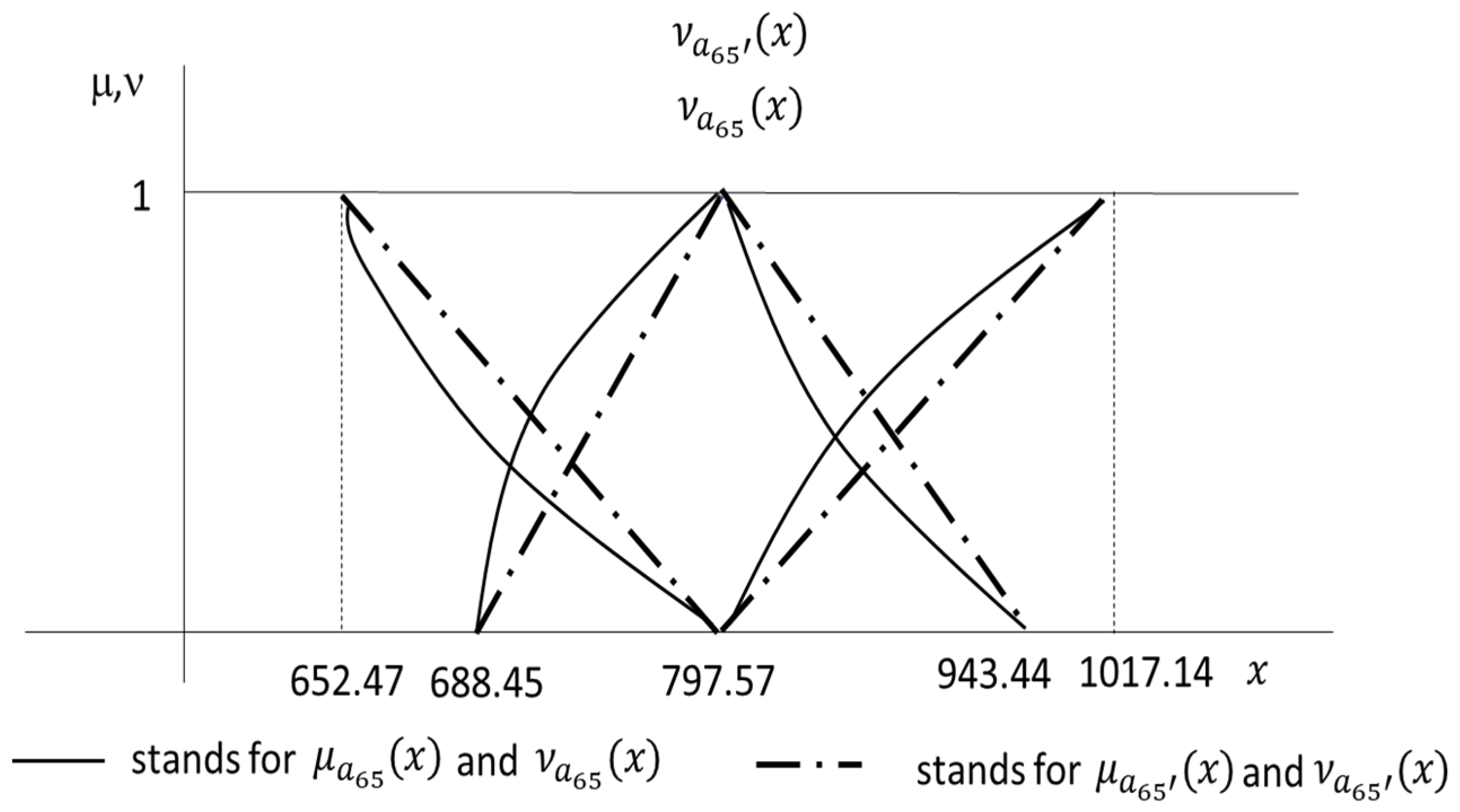
1	0	797.57	797.57	797.57	797.57	82.40	82.40	82.40	82.40
0.75	0.25	767.44	829.95	756.02	843.58	80.12	84.66	79.43	85.30
0.5	0.5	739.34	864.85	718.32	894.83	77.81	86.91	76.39	88.14
0.25	0.75	713.06	902.56	683.94	952.27	75.47	89.13	73.26	90.92
0	1	688.45	943.44	652.47	1017.14	73.11	91.33	70.04	93.65
α	β	${{\underset{\_}{a_{65}}}^{\prime }}_{\alpha }$	${\overline{{a_{65}}^{\prime }}}_{\alpha }$	${{\underset{\_}{a_{65}^{*}}}^{\prime }}_{\beta }$	${\overline{{a_{65}^{*}}^{\prime }}}_{\beta }$	${\underset{\_}{{A_{65}}^{\prime }}}_{\alpha }$	${\overline{{A_{65}}^{\prime }}}_{\alpha }$	${\underset{\_}{{A_{65}^{*}}^{\prime }}}_{\beta }$	${\overline{{A_{65}^{*}}^{\prime }}}_{\beta }$
1	0	797.57	797.57	797.57	797.57	82.40	82.40	82.40	82.40
0.75	0.25	770.29	834.04	761.30	852.46	80.08	84.63	79.31	85.21
0.5	0.5	743.01	870.51	725.02	907.35	77.75	86.87	76.22	88.02
0.25	0.75	715.73	906.97	688.74	962.25	75.43	89.10	73.13	90.83
0	1	688.45	943.44	652.47	1017.14	73.11	91.33	70.04	93.65
α	β	${\underset{\_}{\epsilon }}_{\alpha }$	${\overline{\epsilon }}_{\alpha }$	${\underset{\_}{{\epsilon }^{*}}}_{\beta }$	${\overline{{\epsilon }^{*}}}_{\beta }$	${\underset{\_}{\epsilon }}_{\alpha }$	${\overline{\epsilon }}_{\alpha }$	${\underset{\_}{{\epsilon }^{*}}}_{\beta }$	${\overline{{\epsilon }^{*}}}_{\beta }$
1	0	0	0	0	0	0	0	0	0
0.75	0.25	0.0037	0.0049	0.0070	0.0105	0.0005	0.0003	0.0015	0.0010
0.5	0.5	0.0050	0.0065	0.0093	0.0140	0.0007	0.0004	0.0022	0.0013
0.25	0.75	0.0037	0.0049	0.0070	0.0105	0.0005	0.0003	0.0018	0.0009
0	1	0	0	0	0	0	0	0	0
		$\underset{\_}{\epsilon }$ = 0.00248 $\overline{\epsilon }$ = 0.00327 $\epsilon$ = 0.00288		$\underset{\_}{{\epsilon }^{*}}$ = 0.00466 $\overline{{\epsilon }^{*}}$ = 0.00700 ${\epsilon }^{*}=$0.00583		$\underset{\_}{\epsilon }$ = 0.00082 $\overline{\epsilon }$ = 0.00056 $\epsilon$ = 0.00069		$\underset{\_}{{\epsilon }^{*}}$ = 0.00271 $\overline{{\epsilon }^{*}}$ = 0.00166 $\epsilon$ = 0.00218

Note: The present values are expressed in more than 100 monetary units, y, and the measure of errors over unity is calculated using (21)–(24).

Figure 2. Shapes of $\widetilde{A_{65}}$ and its triangular approximation $\widetilde{{A_{65}}^{\prime }}$.

4. Pricing Special-Rate Annuities and Life Settlements with Intuitionistic Fuzzy Parameters

4.1. Obtaining the Periodical Payment of a Substandard Annuity with Intuitionistic Fuzzy Number Parameters

Special-rate or substandard annuities are immediate annuities that, at the commencement of the contract, consider additional pricing factors along with the policyholder’s age and gender (if permissible). These factors result in the augmentation of annuity payments because of diminished life expectancy (Gatzert and Klotzki 2016).

In accordance with Pitacco and Tabakova (2022), based on the severity of impairment (ranging from minor to major), we can distinguish enhanced life annuities, impaired annuities and care annuities. An enhanced life annuity disburses’ income to an individual with a slightly reduced life expectancy attributable to concrete circumstances, such as smoking or adverse sociodemographic status (Drinkwater et al. 2006). The augmentation in annuity benefits (in comparison to a standard-rate life annuity with the same premium) arises predominantly from the utilization of a higher mortality assumption in specific life tables. Conversely, an impaired life annuity yields a higher income than an enhanced life annuity, reflecting health conditions that significantly curtail the annuitant’s LE (e.g., diabetes, chronic asthma, and cancer). Finally, care annuities target individuals, typically those of advanced age, with severe impairments or individuals already in a state of senescent disability (or long-term care).

Therefore, for a whole-life substandard annuity that is underwritten with a single premium $\mathsf{\Pi }$ by a person with age $x$, the annual payment $C_x$ is

$$C_x\left(i,k,{\mathit{q}}_{\mathit{x}}^{\mathit{S}}\right)=\frac{\mathsf{\Pi }}{a_x\left(i,k,{\mathit{q}}_{\mathit{x}}^{\mathit{S}}\right)}=\frac{\mathsf{\Pi }}{{\sum }_{t=1}^{\mathrm{\infty }}{\left(1+i\right)}^{-t}{\prod }_{j=0}^{t-1}\left(1-\min \left\{1,k·q_{x+j}^S\right\}\right)},$$

(51)

and so $\frac{{\partial C}_x}{\partial i},\frac{{\partial C}_x}{\partial k},\frac{{\partial C}_x}{\partial q_{x+j}^S}\ge 0$.

The interpretation of the discount rate as a technical interest rate, as applicable in the context of substandard annuities, is considered to represent the financial return assured by the company to the policyholder over the long term (Devolder 1988). Eling and Holder (2013) reports that in insurance markets like the United Kingdom, the technical interest rate is established by taking into account the risk-adjusted expected yield of investments. This determination is made with caution, incorporating sufficient margins for adverse deviation and credit risk. It is important to note that the statement provides somewhat ambiguous information, particularly regarding the characterization of the interest rate as “prudent” or “sufficient” and the potential lack of knowledge concerning the evolution of investment yields over extended periods. Lemaire (1990) justifies the adoption of a fuzzified interest rate as a “partial measure of our ignorance” concerning the behavior of interest rates throughout the duration of policies.

In a pension-funding setting, Betzuen et al. (1997) propose, as is common practice, using Fisher’s relationship between the nominal interest rate, real interest rate, and anticipated inflation to fit a fuzzy interest rate. In this regard, Devolder (1988) indicates that the real interest rate must be quantified as “between 2% and 3%” and that anticipated inflation “must be reasonable in the long term.” Although Devolder did not aim to justify the use of fuzzy sets when estimating interest rates, these rules represent imprecisely defined real interest rates and vague anticipated inflation rates.

Thus, let us use the same single premium $\mathsf{\Pi }$ to buy an enhanced annuity for a person aged $x$ and IFN death probabilities $\widetilde{q_x^S}$, mortality multiplier $\widetilde{k,}$ and technical interest $\tilde{i}$. Function (51) and the intuitionistic fuzzy parameters used to evaluate it induce an intuitionistic payment $\widetilde{C_x}$ with $⟨\alpha ,\beta ⟩$-cuts:

$${C_x}_{⟨\alpha ,\beta ⟩}=⟨{C_x}_{\alpha }=\left[{\underset{\_}{C_x}}_{\alpha },{\overline{C_x}}_{\alpha }\right],{C_x^{*}}_{\beta }=\left[{\underset{\_}{C_x^{*}}}_{\beta },{\overline{C_x^{*}}}_{\beta }\right],0\le \alpha +\beta \le 1,\mathsf{\alpha },\beta \in (0,1)⟩,$$

Note that the annuity payment increases with the discount rate, mortality multiplier, and standard mortality probability. Thus, ${C_x}_{⟨\alpha ,\beta ⟩}$ is obtained by evaluating (51) using rules (6)–(9).

$${\underset{\_}{C_x}}_{\alpha }=C_x\left({\underset{\_}{i}}_{\alpha },{\underset{\_}{k}}_{\alpha },{\underset{\_}{{\mathit{q}}_{\mathit{x}}^{\mathit{S}}}}_{\mathit{\alpha }}\right)=\frac{\mathsf{\Pi }}{{\overline{a_x}}_{\alpha }}, {\overline{C_x}}_{\alpha }=C_x\left({\overline{i}}_{\alpha },{\overline{k}}_{\alpha },{\overline{{\mathit{q}}_{\mathit{x}}^{\mathit{S}}}}_{\mathit{\alpha }}\right)=\frac{\mathsf{\Pi }}{{\underset{\_}{a_x}}_{\alpha }},$$

(52)

$${\underset{\_}{C_x^{*}}}_{\beta }=C_x\left({\underset{\_}{i}}_{\beta }^{*},{\underset{\_}{k^{*}}}_{\beta },{\underset{\_}{{\mathit{q}}_{\mathit{x}}^{\mathit{S}\mathbf{*}}}}_{\mathit{\beta }}\right)=\frac{\mathsf{\Pi }}{{\overline{a_x^{*}}}_{\beta }}, {\overline{C_x^{*}}}_{\beta }=C_x\left({\overline{i^{*}}}_{\beta },{\overline{k^{*}}}_{\beta },{\overline{{\mathit{q}}_{\mathit{x}}^{\mathit{S}\mathbf{*}}}}_{\mathit{\beta }}\right)=\frac{\mathsf{\Pi }}{{\underset{\_}{a_x^{*}}}_{\beta }}.$$

(53)

In the case where the standard one-year death probabilities, mortality multiplier, and discount rate are estimated by the TIFN, $\widetilde{C_x}$ allows a linear approximation (13)–(14):

$$\widetilde{C_x}\approx {\widetilde{C_x}}^{\prime }=⟨\left(C_x^{\left(l\right)},C_x^{\left(c\right)},C_x^{\left(r\right)}\right), \left(C_x^{\left(l\right)*},C_x^{\left(c\right)},C_x^{\left(r\right)*}\right)⟩.$$

Note that the premium $\mathsf{\Pi }$ can be considered a TIFN $\tilde{\mathsf{\Pi }}=⟨\left(\mathsf{\Pi },\mathsf{\Pi },\mathsf{\Pi }\right), \left(\mathsf{\Pi },\mathsf{\Pi },\mathsf{\Pi }\right)⟩$ and that $\widetilde{a_x}=\widetilde{{a_x}^{\prime }}$ in (49). Thus, by applying (14),

$${\widetilde{C_x}}^{\prime }=⟨\left(\frac{\mathsf{\Pi }}{a_x^{\left(r\right)}},\frac{\mathsf{\Pi }}{a_x^{\left(c\right)}},\frac{\mathsf{\Pi }}{a_x^{\left(l\right)}}\right), \left(\frac{\mathsf{\Pi }}{a_x^{\left(r\right)*}},\frac{\mathsf{\Pi }}{a_x^{\left(c\right)}},\frac{\mathsf{\Pi }}{a_x^{\left(l\right)*}}\right)⟩.$$

(54)

Example 3. 

We fit the intuitionistic fuzzy number of the annuity payment for two individuals aged  $x=65, 70$ years and a single premium $\Pi =1000$. We use the same baseline mortality table, mortality multiplier, and technical interest rate as in Example 2. Table 4 displays the < $\alpha ,$1-$\alpha$>-cuts, $\alpha$ = 0, 0.25, 0.5, 0.75, and 1 for $\widetilde{C_{65}}$ and $\widetilde{C_{70}}$ and their TIFN approximations $\widetilde{{C_{65}}^{\prime }}$ and $\widetilde{{C_{70}}^{\prime }}$. It can be verified that if the initial data are expressed by means of TIFNs, the approximation to $\widetilde{C_x}$, ${\widetilde{C_x}}^{\prime }$ provides a practically perfect fit. The greatest errors were obtained over ${\underset{\_}{C_{70}^{*}}}_{\beta }$ and ${\overline{C_{70}^{*}}}_{\beta }$, which, in any case, were on average only 0.05%. Figure 3 depicts the shape of  $\widetilde{C_{70}}$calculated using (52)–(53) and its linear approximation (54),  ${\widetilde{C_{70}}}^{\prime }$. The Appendix A shows a pseudocode linked with the calculations in this example.

Table 4. $⟨\alpha ,\beta ⟩$-cuts of $\widetilde{C_{65}}$ and $\widetilde{C_{70}}$, their triangular approximations $\widetilde{C_{70}}$ and $\widetilde{{C_{70}}^{\prime }}$ and the measurement of the approximation errors.

		$\widetilde{{\mathit{C}}_{\mathbf{65}}}$				$\stackrel{~}{{{\mathit{C}}_{\mathbf{70}}}^{\mathbf{\prime }}}$
α	β	${\underset{\_}{C_{65}}}_{\alpha }$	${\overline{C_{65}}}_{\alpha }$	${\underset{\_}{C_{65}^{*}}}_{\beta }$	${\overline{C_{65}^{*}}}_{\beta }$	${\underset{\_}{C_{70}}}_{\alpha }$	${\overline{C_{70}}}_{\alpha }$	${\underset{\_}{C_{70}^{*}}}_{\beta }$	${\overline{C_{70}^{*}}}_{\beta }$
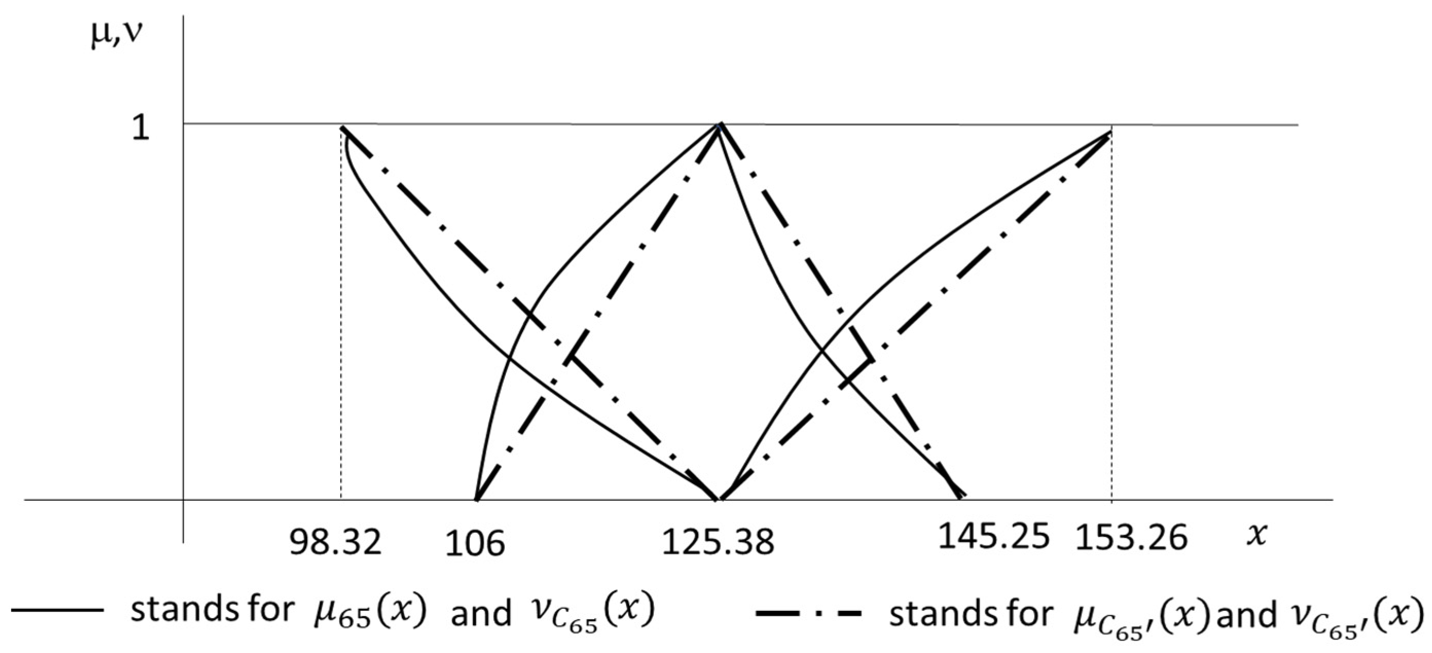
1	0	125.38	125.38	125.38	125.38	167.87	167.87	167.87	167.87
0.75	0.25	120.49	130.30	118.54	132.27	161.33	174.46	158.59	177.24
0.5	0.5	115.63	135.26	111.75	139.21	154.83	181.09	149.39	186.69
0.25	0,75	110.80	140.24	105.01	146.21	148.38	187.78	140.26	196.24
0	1	106.00	145.25	98.32	153.26	141.97	194.51	131.20	205.89
α	β	${{\underset{\_}{C_{65}}}^{\prime }}_{\alpha }$	${\overline{{C_{65}}^{\prime }}}_{\alpha }$	${{\underset{\_}{C_{65}^{*}}}^{\prime }}_{\beta }$	${\overline{{C_{65}^{*}}^{\prime }}}_{\beta }$	${{\underset{\_}{C_{70}}}^{\prime }}_{\alpha }$	${\overline{{C_{70}}^{\prime }}}_{\alpha }$	${{\underset{\_}{C_{70}^{*}}}^{\prime }}_{\beta }$	${\overline{{C_{70}^{*}}^{\prime }}}_{\beta }$
1	0	125.38	125.38	125.38	125.38	167.87	167.87	167.87	167.87
0.75	0.25	120.53	130.35	118.61	132.35	161.39	174.53	158.70	177.37
0.5	0.5	115.69	135.32	111.85	139.32	154.92	181.19	149.54	186.88
0.25	0.75	110.84	140.29	105.08	146.29	148.44	187.85	140.37	196.38
0	1	106.00	145.25	98.32	153.26	141.97	194.51	131.20	205.89
α	β	${\underset{\_}{\epsilon }}_{\alpha }$	${\overline{\epsilon }}_{\alpha }$	${\underset{\_}{{\epsilon }^{*}}}_{\beta }$	${\overline{{\epsilon }^{*}}}_{\beta }$	${\underset{\_}{\epsilon }}_{\alpha }$	${\overline{\epsilon }}_{\alpha }$	${\underset{\_}{{\epsilon }^{*}}}_{\beta }$	${\overline{{\epsilon }^{*}}}_{\beta }$
1	0	0	0	0	0	0	0	0	0
0.75	0.25	0.00038	0.00035	0.00061	0.00061	0.00041	0.00041	0.00073	0.00077
0.5	0.5	0.00052	0.00045	0.00085	0.00078	0.00057	0.00052	0.00101	0.00099
0.25	0.75	0.00041	0.00033	0.00066	0.00056	0.00044	0.00038	0.00078	0.00071
0	1	0	0	0	0	0	0	0	0
		$\underset{\_}{\epsilon }$ = 0.00026 $\overline{\epsilon }$ = 0.00023 $\epsilon$ = 0.00024		$\underset{\_}{{\epsilon }^{*}}$ = 0.00042 $\overline{{\epsilon }^{*}}$ = 0.00040 ${\epsilon }^{*}=$ 0.00041		$\underset{\_}{\epsilon }$ = 0.00028 $\overline{\epsilon }$ = 0.00027 $\epsilon$ = 0.00027		$\underset{\_}{{\epsilon }^{*}}$ = 0.00050 $\overline{{\epsilon }^{*}}$ = 0.00050 ${\epsilon }^{*}=$ 0.00050

Note: The annuity payment is calculated using a pure premium of 1000 monetary units and errors over unity and using (21)–(24).

Figure 3. Shapes of $\widetilde{C_{65}}$ and its triangular approximation $\widetilde{{C_{65}}^{\prime }}$.

Example 4. 

In this example, we show that the proposed methodology produces results that, even though the interpretation and mathematical foundation may differ from the introduction of parameters randomly, are also interpretable in a similar way in decision making. An example of random quantification of mortality parameters can be found, for instance, in Xu and Hoesch (2018).

We quantify $k$ and $i$ through random variables coherent with the fuzzy estimation of Example 3 (see, in this regard, Dubois et al. 2004). Since $\tilde{k}$ and $\tilde{i}$ are symmetric, the multiplier of mortality and the interest rate can be considered Gaussian random variables, which we denote as $k$ and $i$, respectively. Their means will be the core of $\tilde{k}$, which is 6, and the core of $\tilde{i}$, which is 0.02. Additionally, given that the spreads of the nonmembership functions $\tilde{k}$ (1.5) and $\tilde{i}$ (0.0125) mark those values with absolute nonmembership, we assume that they correspond to 3-times the standard deviation of $k$ and $i$, where “real” values of Gaussian random variables tend to be limited. Thus, for $k$, the standard deviation σ would arise from 3$\sigma$ = 1.5, so $\sigma$ = 0.5. Similarly, for $i$, the standard deviation arises from 3$\sigma$ = 0.0125; thus, $\sigma$ = 0.0041667.

We find the random variable amount of income for a person of age $x$ = 65 from (23) through Monte Carlo simulation with 20,000 scenarios. In the simulations, the multiplier and the interest rate are assumed to be uncorrelated. The results are presented in Table 5.

Table 5. Confidence intervals for the annuity payments for a person aged 65 years under the hypothesis that the mortality multiplier and technical interest rates are random variables $k~N\left(\mathrm{6,0.5}\right)$ and $i~N(0.02, 0.0041667)$.

	Values (x)		Membership		Nonmembership		Indeterminacy
	LE	UE	${\mathit{\mu }}_{{{\mathit{C}}_{\mathbf{65}}}^{\mathbf{\prime }}}\mathbf{\left(}\mathit{x}\mathbf{\right)}$		${\mathit{\nu }}_{{{\mathit{C}}_{\mathbf{65}}}^{\mathbf{\prime }}}\mathbf{\left(}\mathit{x}\mathbf{\right)}$		${\mathit{h}}_{{{\mathit{C}}_{\mathbf{65}}}^{\mathbf{\prime }}}\mathbf{\left(}\mathit{x}\mathbf{\right)}$
Median	125.45	125.45	1.00	1.00	0.00	0.00	0.00	0.00
50%CI	120.87	129.93	0.77	0.77	0.17	0.16	0.06	0.07
90%CI	114.36	136.46	0.43	0.44	0.41	0.40	0.16	0.16
95%CI	112.20	138.70	0.32	0.33	0.49	0.48	0.19	0.19
99%CI	108.09	143.41	0.11	0.09	0.64	0.65	0.25	0.26
99.99%CI	102.33	151.42	0.00	0.00	0.85	0.93	0.15	0.07

Notes: (a) LE stands for the lower extreme of the confidence interval, and UE stands for the upper extreme. (b) The spreads of the nonmembership functions $\tilde{k}$ (1.5) and $\tilde{i}$ (0.0125) are 3 times the standard deviation of the Gaussian random variables $k$ and $i$. (c) X% CI stands for the confidence interval at that probability level.

Table 5 shows that the 99.99% confidence interval (CI) [102.33, 151.42] is very similar to ${C_{65}^{*}}_0$ = [98.32, 153.26], as shown in Table 4. In the case of statistical estimation, this CI can be interpreted as all possible outcomes for income. Similarly, ${C_{65}^{*}}_0$ corresponds to values whose nonmembership is not total or, according to Dubois and Prade (2012), those values that are “potentially” possible. From a statistical point of view, the 99% CI in Table 5, [108.09, 143.41], is the set of all possible outcomes once 1% of the most extreme scenarios are excluded because they are “unlikely.” Its intuitionistic correspondence is ${C_{65}}_0$ = [106, 145.25] in Table 4, which contains all values that are “truly” possible (Dubois and Prade 2012). As expected, we can observe that the medians of the Monte Carlo simulations and the core IFN are practically identical.

Table 5 also indicates the level of membership and nonmembership of stochastically simulated scenarios. That is, we can interpret stochastically generated scenarios with intuitionistic logic instruments. For example, for the median, the level of membership is complete, and the level of nonmembership is completely nonexistent, which is entirely expected. We can also assess the level of membership and nonmembership of any other confidence interval. The set of estimates collected by the 50% CI is bounded by the 25th percentile at the lower end (120.87) and the 75th percentile (129.93) at the upper end. At the 25th percentile, ${\mu }_{C_{65}}\left(120.87\right)=0.77$, ${\nu }_{C_{65}}\left(120.87\right)=0.17$ and $h_{C_{65}}\left(120.87\right)=0.06$; at the 75th percentile, ${\mu }_{C_{65}}\left(129.93\right)=0.77$, ${\nu }_{C_{65}}\left(120.87\right)=0.16$ and $h_{C_{65}}\left(120.87\right)=0.07$.

4.2. Pricing Life Settlements with Intuitionistic Fuzzy Number Parameters

In a life settlement, policyholders sell their life-contingent insurance payments to investors as lump sums. The price is determined through an individualized estimation of survival probabilities by the life insurance provider, along with a specific IRR (Braun and Xu 2020). All else being equal, a life-settlement company offers a higher payment for life insurance policy with a shorter estimated LE. This is because, on average, survival-contingent premiums must be paid for a shorter period, where the death benefit is disbursed sooner (Bauer et al. 2020).

Within the concept of life settlement, it is essential to distinguish between virological settlements associated with terminal illness and those in which the policyholder does not necessarily suffer from an excessively severe impairment (Gatzert 2010). Engaging in these types of transactions is beneficial for all participants. Policyholders with impaired LE receive a higher price than the surrender value in the early cancellation of their policies. Through LSs and the bonds derived from their securitization, investors have alternative assets to invest in, whose returns are uncorrelated with those of conventional financial assets such as stocks and bonds. Finally, from the insurance companies’ perspective, investing in LSs can cover the longevity risk associated with life insurance contract liabilities (Kung et al. 2021).

The price of a life settlement on whole-life insurance for a policyholder aged $x$, ${PLS}_x$, comes from the difference between the expected value of the death benefit and the stream of premiums. In this regard, among the existing approaches to price-life settlements, the most common is the probabilistic method, which uses conventional actuarial life mathematics (Brockett et al. 2013):

$$\begin{array}{c}{PLS}_x{=PLS}_x\left(i,k,{\mathit{q}}_{\mathit{x}}^{\mathit{S}}\right)={\displaystyle \sum _{t=0}^{\mathrm{\infty }}}{C}_{x+t}{\left(1+i\right)}^{-(t+1)}{}_{t}p_x·q_{x+t}-{\displaystyle \sum _{t=1}^{\mathrm{\infty }}}{P}_{x+t}{\left(1+i\right)}^{-t}{}_{t}p_x\\ ={\displaystyle \sum _{t=0}^{\mathrm{\infty }}}{C_{x+t}\left(1+i\right)}^{-t}{\displaystyle \prod _{j=0}^{t-1}}\left(1-\min \left\{1,k·q_{x+j}^S\right\}\right)·\min \left\{1,k·q_{x+t}^S\right\}\\ -{\displaystyle \sum _{t=1}^{\mathrm{\infty }}}{P}_{x+t}·{\left(1+i\right)}^{-t}{\displaystyle \prod _{j=0}^{t-1}}\left(1-\min \left\{1,k·q_{x+j}^S\right\}\right),\end{array}$$

(55)

where $C_{x+t}$ $t=0, 1,\dots ,\infty$ and is the death benefit if the insured person died at age $x+t, t$ = 1, 2,…,. ∞ and $P_{x+t}$ is the premium payable at age $x+t$. Thus, if $C_{x+t}$ and $P_{x+t}$ are constant, $C$ and $P$, we find that

$${PLS}_x\left(i,k,{\mathit{q}}_{\mathit{x}}^{\mathit{S}}\right)=C·A_x\left(i,k,{\mathit{q}}_{\mathit{x}}^{\mathit{S}}\right)-P·a_x\left(i,k,{\mathit{q}}_{\mathit{x}}^{\mathit{S}}\right).$$

(56)

and notice that $\frac{{\partial PLS}_x}{\partial k},\frac{{\partial PLS}_x}{\partial q_{x+j}^S}\ge 0$ and $\frac{{\partial PLS}_x}{\partial i}\le 0$.

Establishing an IRR in the valuation of LSs requires setting an interest rate much higher than the technical interest rate at which the insurer would value the policy. This interest rate is obtained by augmenting the risk-free interest rate by adding a premium to the investor’s assumed risk. According to an empirical study of the U.S. life-settlement market by Braun and Xu (2020), this premium can be decomposed into longevity risk (approximately 75%), premium risk (approximately 10%), and default risk (over 6%). One way to estimate this interest rate is to use recently concluded LSs with similar characteristics as a reference. This approach is the so-called neighborhood method (AA-Partners Ltd. 2017). While AA-Partners Ltd. (2017) reduced the set of IRRs used as a benchmark to a crisp value, Andrés-Sánchez and González-Vila (2023) proposed quantifying this set of crisp points as a TFN that retains more information than a single real value.

A common approach used to obtain the IRR involves adjusting the yield spread using regression methods, which depend on proxy variables for the risks faced by investors in life insurance policies (Braun and Xu 2020; Kung et al. 2021). The analytical frameworks provided by these regression models can be leveraged to implement fuzzy regression. This tool has been applied in other actuarial contexts, such as adjusting mortality laws (Koissi and Shapiro 2006; Szymański and Rossa 2021) and claim reserving (Apaydin and Baser 2010; Woundjiagué et al. 2019). Of course, these approaches would yield fuzzy predictions for yield spread. Alternatively, the original econometric models of Braun and Xu (2020) and Kung et al. (2021) produce predictions through probabilistic confidence intervals that can be used to fit an FN representation by means of a probability–possibility transformation (Adjenughwure and Papadopoulos 2020; Al-Kandari et al. 2020), which may be the basis for inducing intuitionistic quantifications by Definition 7 and Remark 7.

In the case of life settlements, if they are evaluated as IFN $\widetilde{q_x^S}$, $\widetilde{k,}$ or $\tilde{i}$, the price for a policyholder aged $x$ years ${\widetilde{PLS}}_x$ is an IFN whose $⟨\alpha ,\beta ⟩-$ cuts are denoted as:

$${{PLS}_x}_{⟨\alpha ,\beta ⟩}=⟨{{PLS}_x}_{\alpha }=\left[{\underset{\_}{{PLS}_x}}_{\alpha },{\overline{{PLS}_x}}_{\alpha }\right],{{PLS}_x^{*}}_{\beta }=\left[{\underset{\_}{{PLS}_x^{*}}}_{\beta },{\overline{{PLS}_x^{*}}}_{\beta }\right],0\le \alpha +\beta \le 1,\mathsf{\alpha },\beta \in \left[0,1\right]⟩,$$

that, in the case of variable death benefits and periodical premiums, can be obtained from (55) by using rules (6)–(9) and considering that the price of an LS decreases with respect to the discount rate and increases with respect to the one-year death probabilities and the mortality multiplier:

$${\underset{\_}{{PLS}_x}}_{\alpha }=\sum _{t=0}^{\infty }{C}_{x+t}{\left(1+{\overline{i}}_{\alpha }\right)}^{-(t+1)}{\overline{{}_{t}p_x}}_{\alpha }·{\underset{\_}{q_{x+t}}}_{\alpha }-\sum _{t=1}^{\infty }{P}_{x+t}{\left(1+{\overline{i}}_{\alpha }\right)}^{-t}{\overline{{}_{t}p_x}}_{\alpha }$$

(57)

$${\overline{{PLS}_x}}_{\alpha }=\sum _{t=1}^{\infty }{C}_{x+t}{\left(1+{\underset{\_}{i}}_{\alpha }\right)}^{-(t+1)}{\underset{\_}{{}_{t}p_x}}_{\alpha }·{\overline{q_{x+t}}}_{\alpha }-\sum _{t=1}^{\infty }{P}_{x+t}{\left(1+{\underset{\_}{i}}_{\alpha }\right)}^{-t}{\underset{\_}{{}_{t}p_x}}_{\alpha },$$

(58)

$${\underset{\_}{{PLS}_x^{*}}}_{\beta }=\sum _{t=1}^{\infty }{C}_{x+t}{\left(1+{\overline{i^{*}}}_{\beta }\right)}^{-(t+1)}{\overline{{}_t{p}_x^{*}}}_{\beta }·{\underset{\_}{q_{x+t}^{*}}}_{\beta }-\sum _{t=1}^{\infty }{P}_{x+t}{\left(1+{\overline{i^{*}}}_{\beta }\right)}^{-t}{\overline{{}_t{p}_x^{*}}}_{\beta },$$

(59)

$${\overline{{PLS}_x^{*}}}_{\beta }=\sum _{t=1}^{\infty }{C}_{x+t}{\left(1+{\underset{\_}{i}}_{\beta }^{*}\right)}^{-(t+1)}{\underset{\_}{{}_t{p}_x^{*}}}_{\beta }·{\overline{q_{x+t}^{*}}}_{\beta }-\sum _{t=1}^{\infty }{P}_{x+t}{\left(1+{\underset{\_}{i}}_{\beta }^{*}\right)}^{-t}{\underset{\_}{{}_t{p}_x^{*}}}_{\beta }.$$

(60)

In the case of constant benefit and pending premiums (56), (57)–(60) become:

$${\underset{\_}{{PLS}_x}}_{\alpha }={C·A}_x\left({\overline{i}}_{\alpha },{\underset{\_}{k}}_{\alpha },{\underset{\_}{{\mathit{q}}_{\mathit{x}}^{\mathit{S}}}}_{\mathit{\alpha }}\right)-{P·a}_x\left({\overline{i}}_{\alpha },{\underset{\_}{k}}_{\alpha },{\underset{\_}{{\mathit{q}}_{\mathit{x}}^{\mathit{S}}}}_{\mathit{\alpha }}\right),$$

(61)

$${\overline{{PLS}_x}}_{\alpha }=C·A_x\left({\underset{\_}{i}}_{\alpha },{\overline{k}}_{\alpha },{\overline{{\mathit{q}}_{\mathit{x}}^{\mathit{S}}}}_{\mathit{\alpha }}\right)-P·a_x\left({\underset{\_}{i}}_{\alpha },{\overline{k}}_{\alpha },{\overline{{\mathit{q}}_{\mathit{x}}^{\mathit{S}}}}_{\mathit{\alpha }}\right),$$

(62)

$${\underset{\_}{{PLS}_x^{*}}}_{\beta }={C·A}_x\left({\overline{i^{*}}}_{\beta },{\underset{\_}{k}}_{\alpha },{\underset{\_}{{\mathit{q}}_{\mathit{x}}^{\mathit{S}\mathit{*}}}}_{\mathit{\beta }}\right)-P·a_x\left({\overline{i^{*}}}_{\beta },{\underset{\_}{k}}_{\alpha },{\underset{\_}{{\mathit{q}}_{\mathit{x}}^{\mathit{S}\mathit{*}}}}_{\mathit{\beta }}\right),$$

(63)

$${\overline{{PLS}_x^{*}}}_{\beta }=C·A_x\left({\underset{\_}{i}}_{\beta }^{*},{\overline{k^{*}}}_{\beta },{\overline{{\mathit{q}}_{\mathit{x}}^{\mathit{S}\mathit{*}}}}_{\mathit{\beta }}\right)-P·a_x\left({\underset{\_}{i}}_{\beta }^{*},{\overline{k^{*}}}_{\beta },{\overline{{\mathit{q}}_{\mathit{x}}^{\mathit{S}\mathit{*}}}}_{\mathit{\beta }}\right).$$

(64)

Suppose that $\widetilde{q_x^S},$ $\tilde{k}$ and $\tilde{i}$ are TIFNs. The estimated price of life insurance policy $\widetilde{{PLS}_x}$ has a linear shape:

$$\widetilde{{PLS}_x}\approx {\widetilde{{PLS}_x}}^{\prime }=⟨\left({PLS}_x^{\left(l\right)},{PLS}_x^{\left(c\right)},{PLS}_x^{\left(r\right)}\right), \left({PLS}_x^{\left(l\right)*},{PLS}_x^{\left(c\right)},{PLS}_x^{{\left(r\right)}^{\prime }*}\right)⟩,$$

whereby applying (15)–(20) in relation (55):

$$\begin{array}{l}{PLS}_x^{\left(l\right)}={PLS}_x\left(i^{\left(r\right)},k^{\left(l\right)},{{\mathit{q}}_{\mathit{x}}^{\mathit{S}}}^{\left(\mathit{l}\right)}\right), {PLS}_x^{\left(c\right)}={PLS}_x\left(i^{\left(c\right)},k^{\left(c\right)},{{\mathit{q}}_{\mathit{x}}^{\mathit{S}}}^{\left(\mathit{c}\right)}\right),\\ {{PLS}_x^{\left(r\right)}={PLS}_x\left(i^{\left(l\right)},k^{\left(r\right)},{{\mathit{q}}_{\mathit{x}}^{\mathit{S}}}^{\left(\mathit{r}\right)}\right),PLS}_x^{\left(l\right)*}={PLS}_x\left(i^{\left(r\right)*},k^{\left(l\right)*},{{\mathit{q}}_{\mathit{x}}^{\mathit{S}}}^{\left(\mathit{l}\right)\mathit{*}}\right), \\ {PLS}_x^{\left(r\right)*}={PLS}_x\left(i^{\left(l\right)*},k^{\left(r\right)*},{{\mathit{q}}_{\mathit{x}}^{\mathit{S}}}^{\left(\mathit{r}\right)\mathit{*}}\right).\end{array}$$

(65)

Example 5. 

We determined the price of a life settlement for two persons aged 65 and 75 years with the same baseline death probabilities and mortality multiplier $\tilde{k}=$ <(5, 6, 7) (4.5, 6, 7.5)>, as in the above numerical applications. The IRR is  $\tilde{i}=$ <(0.11, 0.12, 0.13) (0.105, 0.12, 0.135)>. In both cases, the death benefit is C = 1000 monetary units, pending annual premiums of 14.78 monetary units. Table 6 displays  $⟨\alpha ,\beta ⟩$-cuts for  $⟨\alpha ,1-\alpha ⟩$,  $\alpha$ = 0, 0.25, 0.5. 0.75, 1 of  $\widetilde{{PLS}_{65}}$ and  $\widetilde{{PLS}_{75}}$ and their TIFN approximates  $\widetilde{{{PLS}_{65}}^{\prime }}$ and  $\widetilde{{{PLS}_{75}}^{\prime }}$. Again, we can verify that if the input data are expressed by means of TIFNs, a linear shape approximation to  $\widetilde{{PLS}_x}$,  ${\widetilde{{PLS}_x}}^{\prime }$ provides a practically perfect fit. In all cases, the deviations are less than 0.8%. Figure 4 depicts the shape of  $\widetilde{{PLS}_{65}}$ calculated using (61)–(64) and its linear approximation (65),  $\widetilde{{{PLS}_{65}}^{\prime }}$. In the Appendix A, we present a pseudocode that may help program this numerical application.

Table 6. $⟨\alpha ,\beta ⟩$-cuts of $\widetilde{{PLS}_{65}}$ and $\widetilde{{PLS}_{75}}$, their triangular approximations $\widetilde{{{PLS}_{65}}^{\prime }}$ and ${\widetilde{{PLS}_{75}}}^{\prime }$ and the measurement of the approximation errors. The benefit of life insurance is $C=1000$, and the annual constant premiums are $P=14.78$.

		$\mathbf{Price} \mathbf{of} \mathbf{the} \mathbf{Life} \mathbf{Settlement} \mathbf{(}\mathit{x} \mathbf{=} \mathbf{65}\mathbf{)}$				$\mathbf{Price} \mathbf{of} \mathbf{the} \mathbf{Life} \mathbf{Settlement} \mathbf{(}\mathit{x} \mathbf{=} \mathbf{75}\mathbf{)}$
α	β	${\underset{\_}{{PLS}_{65}}}_{\alpha }$	${\overline{{PLS}_{65}}}_{\alpha }$	${\underset{\_}{{PLS}_{65}^{*}}}_{\beta }$	${\overline{{PLS}_{65}^{*}}}_{\beta }$	${\underset{\_}{{PLS}_{75}}}_{\alpha }$	${\overline{{PLS}_{75}}}_{\alpha }$	${\underset{\_}{{PLS}_{75}^{*}}}_{\beta }$	${\overline{{PLS}_{75}^{*}}}_{\beta }$
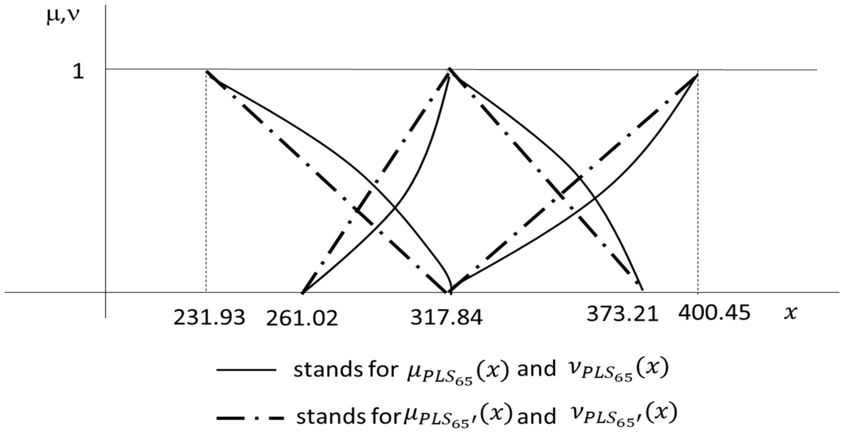
1	0	317.84	317.84	317.84	317.84	597.07	597.07	597.07	597.07
0.75	0.25	303.78	331.80	296.72	338.75	585.46	608.44	579.56	614.05
0.5	0.5	289.63	345.68	275.38	359.48	573.60	619.59	561.48	630.52
0.25	0.75	275.38	359.48	253.79	380.04	561.48	630.52	542.79	646.53
0	1	261.02	373.21	231.93	400.45	549.09	641.25	523.44	662.09
α	β	${\underset{\_}{{{PLS}_{65}}^{\prime }}}_{\alpha }$	${{\overline{{PLS}_{65}}}^{\prime }}_{\alpha }$	${\underset{\_}{{{PLS}_{65}^{*}}^{\prime }}}_{\beta }$	${\overline{{{PLS}_{65}^{*}}^{\prime }}}_{\beta }$	${\underset{\_}{{{PLS}_{75}}^{\prime }}}_{\alpha }$	${\overline{{{PLS}_{75}}^{\prime }}}_{\alpha }$	${\underset{\_}{{{PLS}_{75}^{*}}^{\prime }}}_{\beta }$	${{\overline{{PLS}_{75}^{*}}}^{\prime }}_{\beta }$
1	0	317.84	317.84	317.84	317.84	597.07	597.07	597.07	597.07
0.75	0.25	303.63	331.68	296.36	338.49	585.07	608.11	578.66	613.33
0.5	0.5	289.43	345.52	274.89	359.14	573.08	619.16	560.26	629.58
0.25	0.75	275.22	359.37	253.41	379.80	561.08	630.20	541.85	645.84
0	1	261.02	373.21	231.93	400.45	549.09	641.25	523.44	662.09
α	β	${\underset{\_}{\epsilon }}_{\alpha }$	${\overline{\epsilon }}_{\alpha }$	${\underset{\_}{{\epsilon }^{*}}}_{\beta }$	${\overline{{\epsilon }^{*}}}_{\beta }$	${\underset{\_}{\epsilon }}_{\alpha }$	${\overline{\epsilon }}_{\alpha }$	${\underset{\_}{{\epsilon }^{*}}}_{\beta }$	${\overline{{\epsilon }^{*}}}_{\beta }$
1	0	0	0	0	0	0	0	0	0
0.75	0.25	0.0005	0.0004	0.00121	0.00078	0.0007	0.0005	0.0015	0.0012
0.5	0.5	0.0007	0.0005	0.00180	0.00095	0.0009	0.0007	0.0022	0.0015
0.25	0.75	0.0006	0.0003	0.00151	0.00065	0.0007	0.0005	0.0017	0.0011
0	1	0	0	0	0	0	0	0	0
		$\underset{\_}{\epsilon }$ = 0.00036 $\overline{\epsilon }$ = 0.00023 $\epsilon$ = 0.00030		$\underset{\_}{{\epsilon }^{*}}$ = 0.00093 $\overline{{\epsilon }^{*}}$ = 0.00046 ${\epsilon }^{*}=$ 0.00070		$\underset{\_}{\epsilon }$ = 0.00046 $\overline{\epsilon }$ = 0.00034 $\epsilon$ = 0.00040		$\underset{\_}{{\epsilon }^{*}}$ = 0.00106 $\overline{{\epsilon }^{*}}$ = 0.00077 $\epsilon$ = 0.00092

Note: The errors are referenced over unity by using (21)–(24).

Figure 4. Shapes of $\widetilde{{PLS}_{65}}$ and its triangular approximation $\widetilde{{{PLS}_{65}}^{\prime }}$.

Example 6. 

In this example, again, we quantify  $k$ and$i$ through random variables coherent with the fuzzy estimation of Example 5 (Dubois et al. 2004), similar to that in Example 4. Therefore, $k~N(6,0.5)$ and $i~N(0.12, 0.005)$, where the standard deviation of $i$ is 3$\sigma$ = 0.015. We find the price of the life settlement for a person aged 65 years with (56) through Monte Carlo simulation with 20,000 scenarios. In the simulations, the multiplier and the interest rate are assumed to be uncorrelated. The results are presented in Table 7.)

Table 7. Confidence intervals for the price of life settlement for whole-life insurance in Example 6 for a person aged 65 years under the hypothesis that the mortality multiplier and technical interest rates are random variables $k~N(6,0.5)$ and $i~N(0.12, 0.005)$.

	Values (x)		Membership		Nonmembership		Indeterminacy
	LE	UE	${\mathit{\mu }}_{{{\mathit{P}\mathit{L}\mathit{S}}_{\mathbf{65}}}^{\mathbf{\prime }}}\mathbf{\left(}\mathit{x}\mathbf{\right)}$		${\mathit{\nu }}_{{{\mathit{P}\mathit{L}\mathit{S}}_{\mathbf{65}}}^{\mathbf{\prime }}}\mathbf{\left(}\mathit{x}\mathbf{\right)}$		${\mathit{h}}_{{{\mathit{P}\mathit{L}\mathit{S}}_{\mathbf{65}}}^{\mathbf{\prime }}}\mathbf{\left(}\mathit{x}\mathbf{\right)}$
Median	318.09	318.09	1.00	1.00	0.00	0.00	0.00	0.00
50%CI	304.16	331.77	0.76	0.75	0.16	0.17	0.08	0.08
90%CI	283.01	283.01	0.39	0.39	0.41	0.41	0.21	0.21
95%CI	275.84	357.49	0.26	0.28	0.49	0.48	0.25	0.24
99%CI	263.09	368.84	0.04	0.08	0.64	0.62	0.33	0.30
99.99%CI	235.89	394.97	0.00	0.00	0.95	0.93	0.05	0.07

Notes: (a) LE stands for the lower extreme of the confidence interval, and UE stands for the upper extreme. (b) The spreads of the nonmembership functions $\tilde{k}$ (1.5) and $\tilde{i}$ (0.015) are 3 times the standard deviation of the Gaussian random variables $k$ and $i$. (c) X% CI stands for the confidence interval at that probability level.

Table 7 shows the 99.99% confidence interval (CI) [235.89, 394.97]; all the possible outcomes from a statistical point of view are very similar to ${{PLS}_{65}^{*}}_0$ = [231.93, 400.45], and all the possible potential prices of life settlement are displayed in Table 6. Similarly, whereas the 99% CI in Table 7, [263.39, 368.84], has its intuitionistic correspondence in Table 6 ${{PLS}_{65}}_0=$ [261, 373.21], the median of the random variable prices of the life settlement and the core of IFN are practically identical.

5. Conclusions and Further Research

The parameters necessary for actuarial pricing of life contingencies, such as mortality and the discount rate, are subject to several sources of imprecision and vagueness. This fact has motivated several studies that introduce these sources of uncertainty using fuzzy numbers (FNs). FNs have been applied to model uncertain variables in the field of life insurance (Lemaire 1990; Andrés-Sánchez and González-Vila 2012; Anzilli et al. 2018) as well as in nonlife insurance (Cummins and Derrig 1997; Shapiro 2004). In a more specific context of valuing life contingencies linked to impaired life expectancies (LEs), Andrés-Sánchez et al. (2020) contributed to the field of special-rate annuities, and Aalaei (2022) and Andrés-Sánchez and González-Vila (2023) did so in a life-settlement setting.

Our work extends the results related to the valuation of life contingencies, especially those associated with substandard LEs, under the assumption that information on discount rates and mortality is provided by intuitionistic fuzzy numbers (IFNs). It is worth noting that, to the best of our knowledge, the application of life insurance pricing using parameters estimated through IFNs is novel. Thus, the developments of Kumar and Bajaj (2014), Kahraman et al. (2015), Ersen et al. (2023), and Haktanır and Kahraman (2023) in a capital budgeting setting are extended to actuarial analysis.

The use of FNs in the context of actuarial and financial pricing allows for the introduction of epistemic uncertainty, that is, the perceived reliability of the possible values of the parameters of interest (Dubois and Prade 2012). Therefore, FNs only allow for the introduction of positive information about the feasible values of the parameter. IFNs permit bipolarity to be added by introducing both positive and negative information regarding variables of interest. In other words, this approach involves not only using estimated reliable values of the variable but also using unfeasible values (Dubois and Prade 2012).

We focused on the use of input variables estimated by triangular IFNs (TIFNs) and the approximation of the results obtained with linear shapes. Thus, as indicated by Kreinovich et al. (2020), linear shapes often provide an effective solution for practical applications of fuzzy set theory. The interpretability of results by end users who may not necessarily have knowledge of fuzzy logic (Andrés-Sánchez and González-Vila 2017a; Kreinovich et al. 2020) is a desirable property of using TIFNs. The calculation of the present value of life contingencies with TIFN parameters can be implemented with a very low error by evaluating five scenarios: one considered the maximum reliability scenario and two pairs of extreme positive and negative scenarios. Thus, the results obtained are consistent with those obtained with the application of FNs in financial–actuarial analysis. Although the actuarial functions are nonlinear, the results provide a good triangular approximation in accordance with the literature on fuzzy financial mathematics (Kaufmann 1986; Jiménez and Rivas 1998; Terceño et al. 2003; Heberle and Thomas 2014; Villacorta et al. 2021; Andrés-Sánchez and González-Vila 2023).

These extreme scenarios can be interpreted within the concept of bipolar possibility, as outlined by Dubois and Prade (2012). While the extreme scenarios associated with the values considered in the membership function can be understood as reasonable extreme scenarios, those originating from the nonmembership function admit an interpretation of potential extreme situations. The presented developments can be seamlessly extended to consider a range of values for maximum reliability scenarios instead of just one, using a triangular IFN.

In the numerical tests conducted, we compared the annuity terms and life-settlement prices obtained with IFN parameters to those derived from an estimation through coherent variables in a normal probability–possibility transformation framework (Dubois et al. 2004). We obtained similar results with equivalent interpretations. However, while random modelling requires the generation of a large number of scenarios to estimate statistical confidence intervals, our method allows for parameterizing the variable of interest through an IFN by evaluating only five scenarios. This approach results in clear computational cost savings and enables the interpretation of estimates through a fuzzy-intuitionistic logic perspective.

A natural continuation of this work is the introduction of uncertainty in the analysis of nonlife insurance, extending the results obtained with FN parameters to obtain claim provisions (Andrés-Sánchez 2012; Heberle and Thomas 2016), the discounted value of nonlife insurance liabilities (Cummins and Derrig 1997), and the terminal value of an insurance company (Ungureanu and Vernic 2015) using parameters estimated with IFNs instead of FNs.

The ability to represent gradualness and ontological uncertainty by fuzzy subsets (Dubois and Prade 2012) is also susceptible to its application in life insurance pricing and insurance decision making (Lemaire 1990; Shapiro 2004; Shapiro 2013). Heterogeneity in annuities is commonly introduced by dividing policyholders into relatively broad groups based on generic impairment levels (Anderton and Robb 1998; Olivieri and Pitacco 2016). The use of instruments such as expert systems (Andrés-Sánchez et al. 2020) allows for consideration of the simultaneous membership of a policyholder in more than one group, assigning a level of membership to each of them. For example, if the group of annuitants with standard LE is established for those for whom $k$ = 1, with the next group of annuitants being “slightly impaired” LE ($k$ = 1.1), an annuitant with $k$ = 1.01 essentially belongs to the standard annuitants’ group but must have some membership degree in the “slightly impaired” group.

References

- Aalaei, Mahboubeh. 2022. Pricing life settlements in the secondary market using fuzzy internal rate of return. Journal of Mathematics and Modelling in Finance 2: 53–62. [Google Scholar] [CrossRef]
- AA-Partners Ltd. 2017. AAP Life Settlement Valuation. Retrieved on 10th of September 2022. Available online: https://www.aa-partners.ch/fileadmin/files/Valuation/AAP_Life_Settlement_Valuation_-_Manual_V6.0.pdf (accessed on 30 October 2023).
- Adjenughwure, Kingsley, and Basil Papadopoulos. 2020. Fuzzy-statistical prediction intervals from crisp regression models. Evolving Systems 11: 201–13. [Google Scholar] [CrossRef]
- Al-Kandari, Maryam, Kingsley Adjenughwure, and Kyriakos Papadopoulos. 2020. A Fuzzy-Statistical Tolerance Interval from Residuals of Crisp Linear Regression Models. Mathematics 8: 1422. [Google Scholar] [CrossRef]
- Anderton, W. Nicholas, and Geoffrey H. Robb. 1998. Impaired Lives Annuities. In Medical Selection of Life Risks. London: Palgrave Macmillan UK, pp. 169–71. [Google Scholar]
- Andrés-Sánchez, Jorge de. 2012. Claim reserving with fuzzy regression and the two ways of ANOVA. Applied Soft Computing 12: 2435–41. [Google Scholar] [CrossRef]
- Andrés-Sánchez, Jorge de. 2014. Fuzzy claim reserving in nonlife insurance. Computer Science and Information Systems 11: 825–38. [Google Scholar] [CrossRef]
- Andrés-Sánchez, Jorge de. 2023. Fuzzy Random Option Pricing in Continuous Time: A Systematic Review and an Extension of Vasicek’s Equilibrium Model of the Term Structure. Mathematics 11: 2455. [Google Scholar] [CrossRef]
- Andrés-Sánchez, Jorge de, and Laura González-Vila. 2012. Using fuzzy random variables in life annuities pricing. Fuzzy Sets and Systems 188: 27–44. [Google Scholar] [CrossRef]
- Andrés-Sánchez, Jorge de, and Laura González-Vila. 2017a. Some computational results for the fuzzy random value of life actuarial liabilities. Iranian Journal of Fuzzy Systems 14: 1–25. [Google Scholar] [CrossRef]
- Andrés-Sánchez, Jorge de, and Laura M. González-Vila. 2017b. The valuation of life contingencies: A symmetrical triangular fuzzy approximation. Insurance: Mathematics and Economics 72: 83–94. [Google Scholar] [CrossRef]
- Andrés-Sánchez, Jorge de, and Laura M. González-Vila. 2019. A fuzzy-random extension of the Lee-Carter mortality prediction model. International Journal of Computational Intelligence Systems 12: 775–94. [Google Scholar] [CrossRef]
- Andrés-Sánchez, Jorge de, and Antonio Terceño. 2003. Applications of fuzzy regression in actuarial analysis. Journal of Risk and Insurance 70: 665–99. [Google Scholar] [CrossRef]
- Andrés-Sánchez, Jorge de, and Laura González-Vila. 2023. Life settlement pricing with fuzzy parameters. Applied Soft Computing 148: 110924. [Google Scholar] [CrossRef]
- Andrés-Sánchez, Jorge de, Laura González-Vila, and Aihua Zhang. 2020. Incorporating fuzzy information in pricing substandard annuities. Computers and Industrial Engineering 145: 106475. [Google Scholar] [CrossRef]
- Anzilli, Luca, and Gisella Facchinetti. 2017. New definitions of mean value and variance of fuzzy numbers: An application to the pricing of life insurance policies and real options. International Journal of Approximate Reasoning 91: 96–113. [Google Scholar] [CrossRef]
- Anzilli, Luca, Gisella Facchinetti, and Tommaso Pirotti. 2018. Pricing of minimum guarantees in life insurance contracts with fuzzy volatility. Information Sciences 460: 578–93. [Google Scholar] [CrossRef]
- Apaydin, Aysen, and Furkan Baser. 2010. Hybrid fuzzy least-squares regression analysis in claims reserving with geometric separation method. Insurance: Mathematics and Economics 47: 113–22. [Google Scholar] [CrossRef]
- Atanassov, Krassimir. 1986. Intuitionistic fuzzy sets. Fuzzy Sets and Systems 20: 87–96. [Google Scholar] [CrossRef]
- Atanassov, Krassimir. 1989. More on intuitionistic fuzzy sets. Fuzzy Sets and Systems 33: 37–45. [Google Scholar] [CrossRef]
- Bauer, Daniel, Jochen Russ, and Nan Zhu. 2020. Asymmetric information in secondary insurance markets: Evidence from the life settlements market. Quantitative Economics 11: 1143–75. [Google Scholar] [CrossRef]
- Bayeg, Selami, and Rasiye Mert. 2021. On intuitionistic fuzzy version of Zadeh’s extension principle. Notes on Intuitionistic Fuzzy Sets 27: 9–17. [Google Scholar] [CrossRef]
- Betzuen, Amancio, Mariano Jiménez, and Juan A. Rivas. 1997. Actuarial mathematics with fuzzy parameters: An application to collective pension plans. Fuzzy Economic Review 2: 47–66. [Google Scholar] [CrossRef]
- Bhaumik, Ankar, Sankar K. Roy, and Deng-Feng Li. 2017. Analysis of triangular intuitionistic fuzzy matrix games using robust ranking. Journal of Intelligent and Fuzzy Systems 33: 327–36. [Google Scholar] [CrossRef]
- Boltürk, Eda, and Cengiz Kahraman. 2022. Interval-valued and circular intuitionistic fuzzy present worth analyses. Informatica 33: 693–711. [Google Scholar] [CrossRef]
- Braun, Alexander, and Jiahua Xu. 2020. Fair value measurement in the life settlement market. The Journal of Fixed Income 29: 100–23. [Google Scholar] [CrossRef]
- Brockett, Patrick L., Shuo-li Chuang, Yinglu Deng, and Richard D. MacMinn. 2013. Incorporating longevity risk and medical information into life settlement pricing. Journal of Risk and Insurance 80: 799–826. [Google Scholar] [CrossRef]
- Buckley, James J. 1987. The fuzzy mathematics of finance. Fuzzy Sets and Systems 21: 257–73. [Google Scholar] [CrossRef]
- Buckley, James J. 1992. Solving fuzzy equations in economics and finance. Fuzzy Sets and Systems 48: 289–96. [Google Scholar] [CrossRef]
- Buckley, James J., and Yunxia Qu. 1990. On using α-cuts to evaluate fuzzy equations. Fuzzy Sets and Systems 38: 309–12. [Google Scholar] [CrossRef]
- Bundock, Gary. 2006. Application Processing. In Brackenridge’s Medical Selection of Life Risks. Edited by R. D. C. Brackenridge and W. John Elder. London: Palgrave Macmillan. [Google Scholar]
- Burillo, Pedro, and Humberto Bustince. 1996. Construction theorems for intuitionistic fuzzy sets. Fuzzy Sets and Systems 84: 271–81. [Google Scholar] [CrossRef]
- Cassú, Carles, Pere Planas, Joan Carles Ferrer, and Joan Bonet. 1996. Accumulated capital for the retirement plans in fuzzy finance mathematics. Fuzzy Economic Review 1: 83–92. [Google Scholar] [CrossRef]
- Couso, Inés, Susana Montes, and Pedro Gil. 2001. The necessity of the strong α-cuts of a fuzzy set. International Journal of Uncertain Fuzziness Knowledge-Based Systems 2: 249–62. [Google Scholar] [CrossRef]
- Cummins, David J., and Richard A. Derrig. 1997. Fuzzy financial pricing of property-liability insurance. North American Actuarial Journal 1: 21–40. [Google Scholar] [CrossRef]
- Derrig, Richard A., and Kristoff M. Ostaszewski. 1997. Managing the tax liability of a property-liability insurance company. Journal of Risk and Insurance 64: 695–711. [Google Scholar] [CrossRef]
- Derrig, Richard A., and Kristoff M. Ostaszewski. 2006. Fuzzy Set Theory. In Encyclopedia of Actuarial Science. Edited by Josef L. Teugels, Bjorn Sundt and Soren Asmussen. Chichester: John Willey and Sons Ltd. [Google Scholar] [CrossRef]
- Devolder, Pierre. 1988. Le taux d’actualization en assurance. Geneva Papers on Risk and Insurance 13: 265–72. [Google Scholar] [CrossRef]
- Dębicka, Joanna, Stanislaw Heilpern, and Agnieszka Marciniuk. 2022. Modelling Marital Reverse Annuity Contract in a Stochastic Economic Environment. Statistika: Statistics and Economy Journal 102: 261–81. [Google Scholar] [CrossRef]
- Dong, Ming-Gao, and Shou-Yi Li. 2016. Project investment decision making with fuzzy information: A literature review of methodologies based on taxonomy. Journal of Intelligent and Fuzzy Systems 30: 3239–52. [Google Scholar] [CrossRef]
- Dong, Weimin, and Haresh C. Shah. 1987. Vertex method for computing functions of fuzzy variables. Fuzzy Sets and Systems 24: 65–78. [Google Scholar] [CrossRef]
- Drinkwater, Matthew, Joseph E. Montminy, Eric T. Sondergeld, Christopher G. Raham, and Chad R. Runchey. 2006. Substandard annuities. Technical Report. LIMRA International Inc. and the Society of Actuaries, in Collaboration with Ernst & Young LLP. Available online: https://www.soa.org/Files/Research/007289-Substandard-annuities-full-rpt-REV-8-21.pdf (accessed on 10 October 2023).
- Dubois, Didier, and Henry Prade. 1993. Fuzzy numbers: An overview. Readings in Fuzzy Sets for Intelligent Systems, 112–48. [Google Scholar] [CrossRef]
- Dubois, Didier, and Henry Prade. 2012. Gradualness, uncertainty and bipolarity: Making sense of fuzzy sets. Fuzzy Sets and Systems 192: 3–24. [Google Scholar] [CrossRef]
- Dubois, Didier, Laurent Folloy, Gilles Mauris, and Henry Prade. 2004. Probability–possibility transformations, triangular fuzzy sets, and probabilistic inequalities. Reliable Computing 10: 273–97. [Google Scholar] [CrossRef]
- Eling, Martin, and Stefan Holder. 2013. Maximum technical interest rates in life insurance in Europe and the United States: An overview and comparison. The Geneva Papers on Risk and Insurance-Issues and Practice 38: 354–75. [Google Scholar] [CrossRef]
- Ersen, Huseyin Y., Oktay Tas, and Cengit Kahraman. 2018. Intuitionistic fuzzy real-options theory and its application to solar energy investment projects. Engineering Economics 29: 140–50. [Google Scholar] [CrossRef]
- Ersen, Huseyin Y., Oktay Tas, and Umut Ugurlu. 2023. Solar Energy Investment Valuation With Intuitionistic Fuzzy Trinomial Lattice Real Option Model. IEEE Transactions on Engineering Management 70: 2584–93. [Google Scholar] [CrossRef]
- Gatzert, Nadine. 2010. The secondary market for life insurance in the UnitedKingdom, Germany, and the United States: Comparison and overview. Risk Management and Insurance Review 13: 279–301. [Google Scholar] [CrossRef]
- Gatzert, Nadine, and Udo Klotzki. 2016. Enhanced annuities: Drivers of and barriers to supply and demand. The Geneva Papers on Risk and Insurance-Issues and Practice 41: 53–77. [Google Scholar] [CrossRef]
- Goodwin, Linda S., Paul E. Hankwitz, and Martin L. Engman. 2006. Underwriting older ages. In Brackenridge’s Medical Selection of Life Risks. Edited by R. D. C. Brackenridge and W. John Elder. London: Palgrave Macmillan. [Google Scholar]
- Haktanır, Elif, and Cengit Kahraman. 2023. Intuitionistic fuzzy risk adjusted discount rate and certainty equivalent methods for risky projects. International Journal of Production Economics 257: 108757. [Google Scholar] [CrossRef]
- Heberle, Jochen, and Anne Thomas. 2014. Combining chain-ladder claims reserving with fuzzy numbers. Insurance: Mathematics and Economics 55: 96–104. [Google Scholar] [CrossRef]
- Heberle, Jochen, and Anne Thomas. 2016. The fuzzy Bornhuetter–Ferguson method: An approach with fuzzy numbers. Annals of Actuarial Science 10: 303–21. [Google Scholar] [CrossRef]
- Jiménez, Mariano, and Juan A Rivas. 1998. Fuzzy number approximation. International Journal of Uncertainty, Fuzziness and Knowledge-Based Systems 6: 69–78. [Google Scholar] [CrossRef]
- Kahraman, Cengit, Da Ruan, and Ethem Tolga. 2002. Capital budgeting techniques using discounted fuzzy versus probabilistic cash flows. Information Sciences 142: 57–76. [Google Scholar] [CrossRef]
- Kahraman, Cengit, S. Çevik Onar, and Basar Öztayşi. 2015. Engineering economic analyses using intuitionistic and hesitant fuzzy sets. Journal of Intelligent and Fuzzy Systems 29: 1151–68. [Google Scholar] [CrossRef]
- Kaufmann, Arnold. 1986. Fuzzy subsets applications in OR and management. In Fuzzy Sets Theory and Applications. Edited by André Jones, Arnold Kaufmann and Hans Jürgen Zimmermann. Dordrecht: Springer, pp. 257–300. [Google Scholar]
- Kita, Michael W. 2000. The rating of substandard lives. In Medical Selection of Life Risks. London: Palgrave Macmillan UK, pp. 61–88. [Google Scholar]
- Koissi, Marie-Claire, and Arnold F. Shapiro. 2006. Fuzzy formulation of the Lee–Carter model for mortality forecasting. Insurance: Mathematics and Economics 39: 287–309. [Google Scholar] [CrossRef]
- Kreinovich, Vladik, Olga Kosheleva, and Shahnaz N. Shahbazova. 2020. Why Triangular and Trapezoid Membership Functions: A Simple Explanation. In Recent Developments in Fuzzy Logic and Fuzzy Sets. Studies in Fuzziness and Soft Computing. Edited by Shahnaz N. Shahbazova, Michio Sugeno and Janusz Kacprzyk. Cham: Springer, vol. 391. [Google Scholar] [CrossRef]
- Kumar, Gaurav, and Rakesh K. Bajaj. 2014. Implementation of intuitionistic fuzzy approach in maximizing net present value. International Journal of Mathematical and Computational Sciences 8: 1069–73. [Google Scholar] [CrossRef]
- Kumar, P. Senthil, and R. Jahir Hussain. 2015. A method for solving unbalanced intuitionistic fuzzy transportation problems. Notes on Intuitionistic Fuzzy Sets 21: 54–65. [Google Scholar] [CrossRef]
- Kung, Ko-Lun, Mi-Hun Hsieh, Jing-Lung Peng, Chenghsien J. Tsai, and Jennifer L. Wang. 2021. Explaining the risk premiums of life settlements. Pacific-Basin Finance Journal 68: 101574. [Google Scholar] [CrossRef]
- Lee, Ronald D., and Lawrence R. Carter. 1992. Modelling and forecasting US mortality. Journal of the American Statistical Association 87: 659–71. [Google Scholar] [CrossRef]
- Lemaire, Jean. 1990. Fuzzy insurance. ASTIN Bulletin: The Journal of the IAA 20: 33–55. [Google Scholar] [CrossRef]
- Lim, Hong-Beng, and Nariankadu D. Shyamalkumar. 2022. Evaluating Medical Underwriters in Life Settlements: Problem of Unreported Deaths. North American Actuarial Journal 26: 298–322. [Google Scholar] [CrossRef]
- Lubovich, Jandra, Jon Sabes, and Paul Siegert. 2008. Introduction to Methodologies Used to Price Life Insurance Policies in Life Settlement Transactions. SSRN. [Google Scholar] [CrossRef]
- Mahapatra, G. S., and Tapan K. Roy. 2013. Intuitionistic fuzzy number and its arithmetic operation with application on system failure. Journal of Uncertain Systems 7: 92–107. [Google Scholar]
- Meyricke, Ramona, and Michael Sherris. 2013. The determinants of mortality heterogeneity and implications for pricing annuities. Insurance: Mathematics and Economics 53: 379–87. [Google Scholar] [CrossRef]
- Mircea, Iulian, and Michaela Covrig. 2015. A discrete time insurance model with reinvested surplus and a fuzzy number interest rate. Procedia Economics and Finance 32: 1005–11. [Google Scholar] [CrossRef]
- Mitchell, Harvey B. 2004. Ranking-intuitionistic fuzzy numbers. International Journal of Uncertainty, Fuzziness and Knowledge-Based Systems 12: 377–86. [Google Scholar] [CrossRef]
- Muzzioli, Silvia, and Bernard De Baets. 2016. Fuzzy approaches to option price modelling. IEEE Transactions on Fuzzy Systems 25: 392–401. [Google Scholar] [CrossRef]
- Nguyen, Hung T. 1978. A note on the extension principle for fuzzy sets. Journal of Mathematical Analysis and Aplications 64: 369–80. [Google Scholar] [CrossRef]
- Nowak, Piotr, and Maciej Romaniuk. 2017. Catastrophe bond pricing for the two-factor Vasicek interest rate model with automatized fuzzy decision making. Soft Computing 21: 2575–97. [Google Scholar] [CrossRef]
- Olivieri, Annamaria. 2006. Heterogeneity in survival models. Applications to pensions and life annuities. Belgian Actuarial Bulletin 6: 23–39. [Google Scholar] [CrossRef]
- Olivieri, Annamaria, and Ermanno Pitacco. 2016. Frailty and risk classification for life annuity portfolios. Risks 4: 39. [Google Scholar] [CrossRef]
- Ostaszewski, K. 1993. An Investigation into Possible Applications of Fuzzy Sets Methods in Actuarial Science. Schaumburg: Society of Actuaries. [Google Scholar]
- Pitacco, Ermanno. 2017. Life Annuities. Products, Guarantees, Basic Actuarial Models. Available online: https://ssrn.com/abstract=2887359 (accessed on 30 October 2023).
- Pitacco, Ermanno. 2019. Heterogeneity in mortality: A survey with an actuarial focus. European Actuarial Journal 9: 3–30. [Google Scholar] [CrossRef]
- Pitacco, Ermanno, and Daniela Y. Tabakova. 2022. Special-rate life annuities: Analysis of portfolio risk profiles. Risks 10: 65. [Google Scholar] [CrossRef]
- Promislow, S. David. 2014. Fundamentals of Actuarial Mathematics. New York: John Wiley and Sons. [Google Scholar]
- Rasheed, Farah, Sagida Kousar, Javid Shabbir, Nasreen Kausar, Dragan Pamucar, and Yaé Ulrich Gaba. 2021. Use of intuitionistic fuzzy numbers in survey sampling analysis with application in electronic data interchange. Complexity 2021: 9989477. [Google Scholar] [CrossRef]
- Richards, Stephen J. 2008. Applying survival models to pensioner mortality data. British Actuarial Journal 14: 257–303. [Google Scholar] [CrossRef]
- Sfiris, Dimitris S., and Basil K. Papadopoulos. 2014. Nonasymptotic fuzzy estimators based on confidence intervals. Information Sciences 279: 446–59. [Google Scholar] [CrossRef]
- Shapiro, Arnold F. 2004. Fuzzy logic in insurance. Insurance: Mathematics and Economics 35: 399–424. [Google Scholar] [CrossRef]
- Shapiro, Arnold F. 2013. Modelling future lifetime as a fuzzy random variable. Insurance: Mathematics and Economics 53: 864–70. [Google Scholar] [CrossRef]
- Shen, Yonghong, and Wei Chen. 2012. Multivariate extension principle and algebraic operations of intuitionistic fuzzy sets. Journal of Applied Mathematics 845090. [Google Scholar] [CrossRef]
- Sosa, Ivan, and Oscar Montes. 2022. Understanding the InsurTech dynamics in the transformation of the insurance sector. Risk Management Insurance Review 25: 35–68. [Google Scholar] [CrossRef]
- Szymański, Andrzej, and Agnieszka Rossa. 2021. The modified fuzzy mortality model based on the algebra of ordered fuzzy numbers. Biometrical Journal 63: 671–89. [Google Scholar] [CrossRef]
- Terceño, Antonio, Jorge de Andrés-Sánchez, M. Gloria Barberà, and Tomás Lorenzana. 2003. Using fuzzy set theory to analyse investments and select portfolios of tangible investments in uncertain environments. International Journal of Uncertainty, Fuzziness and Knowledge-Based Systems 11: 263–81. [Google Scholar] [CrossRef]
- Ungureanu, Daniela, and Raluca Vernic. 2015. On a fuzzy cash flow model with insurance applications. Decisions in Economics and Finance 38: 39–54. [Google Scholar] [CrossRef]
- Villacorta, Pablo J., Laura M. González-Vila, and Jorge de Andrés-Sánchez. 2021. Fuzzy Markovian Bonus-Malus Systems in Nonlife Insurance. Mathematics 9: 347. [Google Scholar] [CrossRef]
- Werth, Martin. 1995. Preferred Lives––A More Complete Method of Risk Assessment. Staple Inn Actuarial Society. Available online: https://www.actuaries.org.uk/system/files/documents/pdf/preferred.pdf (accessed on 30 October 2023).
- World Cancer Research Fund International. 2023. Cancer Survirval Statistics. Available online: https://www.wcrf.org/cancer-trends/worldwide-cancer-data/ (accessed on 12 January 2024).
- Woundjiagué, Apollinaire, Martin Le Roux Bidima, and Mwangi Ronald Waweru. 2019. A fuzzy least-squares estimation of a hybrid log-poisson regression and its goodness of fit for optimal loss reserves in insurance. International Journal of Fuzzy Systems 21: 930–44. [Google Scholar] [CrossRef]
- Wu, Liang, Jie-fang Liu, Jun-tao Wang, and Ya-ming Zhuang. 2016. Pricing for a basket of LCDS under fuzzy environments. SpringerPlus 5: 1–12. [Google Scholar] [CrossRef]
- Xu, Jiahua. 2020. Dating death: An empirical comparison of medical underwriters in the US life settlement market. North American Actuarial Journal 24: 36–56. [Google Scholar] [CrossRef]
- Xu, Jiahua, and Adrian Hoesch. 2018. Predicting longevity: An analysis of potential alternatives to life expectancy reports. Journal of Investing 27: 65–79. [Google Scholar] [CrossRef]
- Xu, Weidong, Chongfeng Wu, Weijun Xu, and Hongyi Li. 2009. A jump-diffusion model for option pricing under fuzzy environments. Insurance: Mathematics and Economics 44: 337–44. [Google Scholar] [CrossRef]
- Yuan, Xuehai, Hongxing Li, and Cheng Zhang. 2014. The theory of intuitionistic fuzzy sets based on the intuitionistic fuzzy special sets. Information Sciences 277: 284–98. [Google Scholar] [CrossRef]
- Zadeh, Lotfi A. 1965. Fuzzy Sets. Information and Control 8: 338–53. [Google Scholar] [CrossRef]